Chapter 9
Optical Modeling of Colored Materials
There are many applications where it is useful to know the relationship between colorants and their resulting color when mixed. For thousands of years, artisans have used their experiences to develop this relationship for ceramics, textiles, paints, and glass, to name a few. This experience was handed down to the next generation through apprenticeships. Trade guilds, developed during medieval times, exemplify the apprentice approach. The introduction of spectrophotometers capable of measuring opaque samples opened the possibility of using the spectral data to establish a relationship between the materials' spectral properties, concentrations, and the resulting spectra following mixing. Colorimetric coordinates were calculated from the mixture's spectrum, defining the mixture's color. Having established such a relationship, it should be possible to reverse the relationship. This facilitates answering the following questions. What are the concentrations necessary to produce a particular color, that is, predicting a color formula (or recipe)? Are the selected colorants the best colorants to use, either leading to the least amount of metamerism when matching a standard, or the least amount of color inconstancy when the standard is colorimetric? Do the selected colorants minimize color variability caused by process variability? When the batch does not match, how is the formula adjusted to improve the match?
There are several ways to establish the relationship between concentration and color. One way is to derive a spectral‐based theoretical optical model and adjust the model coefficients empirically to maximize accuracy. In some cases, this approach is inadequate and modeling is abandoned. A database is created by producing mixtures where concentration is sampled systematically. The database is used to create a multidimensional lookup table and interpolation is used to calculate a formula for a specific color. The database can also be used as training data to create a neural network or other learning‐based algorithms. In this chapter, we focus on the model‐based approach.
A. GENERIC APPROACH TO COLOR MODELING
Berns (1997) found that many coloration systems could be modeled using a generic, two‐step approach. The first step was discovering a model where the relationship between the color components and spectral data was linear. Discovery took the form of a literature search or a derivation based on first principles. The models we describe come from the literature.
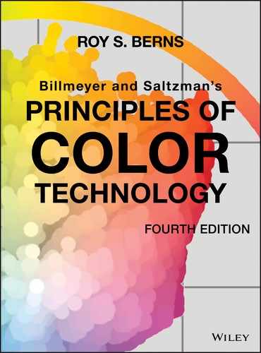
A linear relationship has two requirements. The first is scalability. The spectral data for each colorant should be scalable. This is tested by producing a series of colors where the amount is varied between minimum and maximum. We use the example of a liquid crystal display where spectral radiance was measured of each primary at six different digital values (amounts), shown in Figure 9.1. Scalability is verified when the spectra are coincident following normalization to a single wavelength, shown in Figure 9.2. This means that all the spectra can be predicted by a single spectrum, usually the maximum for displays. This is shown in Eq. (9.1):
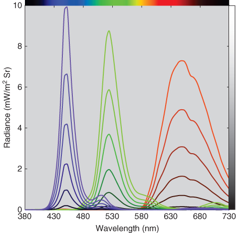
Figure 9.1 Spectral radiance measurements of red, green, and blue primary ramps for a liquid crystal display.

Figure 9.2 Spectral radiance measurements of red, green, and blue primary ramps normalized to each spectrum's peak radiance.
where spectral radiance, Lλ, is predicted from the colorant's maximum spectral radiance, Lλ, max, and effective colorant amount, ce, equivalent to a scalar in linear algebra. The direct measurement of spectral radiance defines the linear model. Scalar ce can be calculated as a ratio at the peak wavelength, the ratio of the integration of the spectrum, or is estimated using least squares linear regression using all the wavelength data.
The second requirement is additivity where a mixture is predicted by the summation of each colorant, shown in Eq. (9.2)
This is verified by predicting mixtures from a linear combination of each colorant's maximum spectral radiance, shown in Eq. (9.3)
Regression is used to estimate effective colorant amount where spectral radiance RMS error is minimized. A comparison of the measured and estimated spectra is shown in Figure 9.3. The spectra are nearly coincident. Spectral differences can also be used as a measure of scalability.
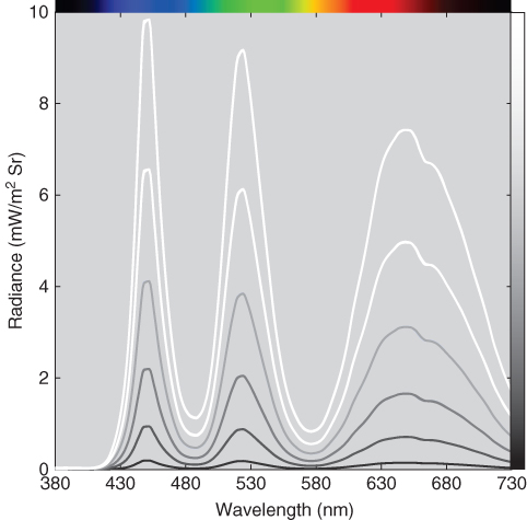
Figure 9.3 Measured (thick lines) and estimated (thin lines) spectral radiance of neutral colors based on Eq. (9.3).
The second step of Berns' generic approach was to discover the relationship between the user controls, digital counts (d) in this example, and effective colorant amount, shown in Eq. (9.4). Discovery took the form of a literature search, a derivation based on first principles, fitting measurement data, or building a one‐dimensional lookup table. The relationship between digital counts and effective colorant amount for the measured liquid‐crystal display is shown in Figure 9.4. This display‐based relationship is referred to as an optoelectronic conversion function, OECF, or tone‐response curve, TRC
Figure 9.4 Nonlinear relationship between digital counts and effective colorant amount for the red primary of a liquid crystal display. Although not plotted, the blue and green primaries have similar relationships.
This generic approach will be used throughout this chapter.
B. MODELING TRANSPARENT MATERIALS
The modeling of transparent materials is subtractive where colorants absorb light. Bouguer (1729) and later Lambert (1760) discovered that spectral transmittance could be transformed using logarithms to achieve a linear system. Experiments were performed using colored glass of different thickness, shown in Figure 9.5. Suppose that a 1 cm thick glass transmitted one half of the light incident upon it at some arbitrary wavelength. It would seem that if the glass was 2 cm thick, it would transmit no light. Each centimeter of material would subtract one half of the light (½–½). However, they instead found that the transmittance was one quarter of the light. If the glass thickness was increased to 3 cm, the transmittance was one eighth of the light. We see that each centimeter of material has an exponential rather than a subtractive effect [¼ = (½)2; ⅛ = (½)3].

Figure 9.5 Bouguer and later Lambert discovered that there was an exponential relationship between thickness and spectral transmittance.
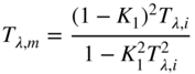
The measured transmittance of the three 1 cm glasses will be slightly less than the single 3 cm glass because there are three times the number of first‐surface reflections at each air and glass interface. We have to account for this difference in order to correctly use the exponential relationship. As we learned in Chapter , the Fresnel formulas are used to “get inside” the glass, that is, calculate internal transmittance, Tλ,i. If we assume that the light strikes the glass along its normal angle, Eqs. (9.5)–(9.7) are used to transform between internal and measured transmittance, Tλ,m:

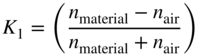
where n is refractive index (Allen 1980). The n of air is 1. For different angles of incidence, Eqs. 1.1, 1.2, 1.3, shown in Chapter 1, are used.
The Bouguer–Lambert law is shown in Eq. (9.8):
where internal transmittance, Tλ,i, depends on the glass' internal transmittance at unit thickness, tλ, and its thickness, b. (Note the deliberate use of upper‐ and lower‐case letters.)
When designing filters for cameras and colorimeters, multiple glasses are glued together. If the refractive index of the glue matches that of the glasses, the total transmittance is a product of the individual glasses, shown in Eq. (9.9) for two filters
About 100 years later, Beer found that the same principles that described the relationship between transmittance and thickness for transparent materials also applied to liquids of varying concentration (Beer 1852, 1854), shown in Figure 9.6. Thus, the linear mixing law for colored materials that do not scatter light is known as the Bouguer–Beer law or Lambert–Beer law.
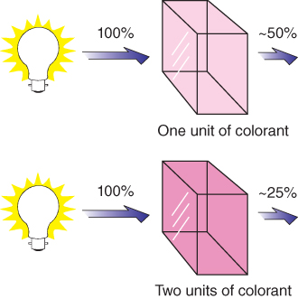
Figure 9.6 Beer discovered that there was an exponential relationship between concentration and spectral transmittance.
The linear model is defined by a logarithmic transformation of internal transmittance, shown in Eq. (9.10):
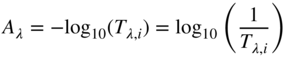
where A defines absorbance. The absorbance of a transparent material depends on its unit absorptivity, aλ, thickness, b, and concentration, c, shown in Eq. (9.11)
Absorptivity is also called an absorption coefficient, k or α, or an extinction coefficient, ε.
A classic experiment in analytical chemistry is to verify Beer's law by dissolving a dye in a solvent at different concentrations and comparing absorbance, usually at the wavelength of maximum absorbance, and concentration. A pair of matched cuvettes is used where the solvent is in one cuvette (“blank”) and the solvent and dye are in the other cuvette. A single‐beam spectrophotometer is calibrated with the blank in the optical path. Cuvettes filled with solvent are placed in both positions when calibrating a double‐beam spectrophotometer. Measurements are directly internal transmittance. A line is fit where absorbance is predicted from concentration. Any deviation from linearity is known as Beer's law failure, reasons including experimental error, measurement imprecision, and changes in the electronic characteristics of the dye molecules at very low and high concentrations.
As an example, a purple polystyrene plastic was molded into sections ranging from 1.00 to 6.00 mm in 1 mm increments and measured with a spectrophotometer, the data shown in Figure 9.7. Transmittance decreases with an increase in thickness. The change, however, is not proportional with thickness.
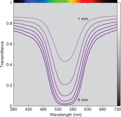
Figure 9.7 Spectral transmittance of polystyrene plastic at varying thickness in 1 mm increments.
Polystyrene has a refractive index that varies from 1.68 at 380 nm to 1.50 at 730 nm. The average, 1.60, was used to calculate a K1 of 0.053 and used to transform to internal transmittance using Eqs. (9.5) and (9.6), the data plotted in Figure 9.8. Internal transmittance always increases compared with measured transmittance.

Figure 9.8 Spectral internal transmittance of polystyrene plastic at varying thickness.
Absorbance was calculated from internal transmittance using Eq. (9.10), the spectra shown in Figure 9.9. Absorbance increases with a decrease in transmittance. Absorbance is proportional to thickness.
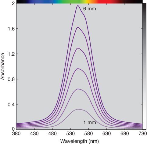
Figure 9.9 Spectral absorbance of polystyrene plastic at varying thickness.
The absorbance at 1 mm was defined as the unit absorptivity. The simplest way to estimate thickness is by dividing the absorbance at 550 nm for each spectrum by the unit absorptivity, the results shown in Figure 9.10 and Table 9.1. There is a slight amount of error for the thickest sample, likely caused by measurement imprecision. Alternatively, least squares linear regression can be used to estimate thickness using all the wavelengths where spectral absorbance RMS error is minimized. This resulted in an accurate estimation of thickness.

Figure 9.10 Measured and estimated thickness using absorbance at 550 nm (green line), absorbance using all wavelengths (black line), “absorbance” ignoring first surface reflections at 550 nm (red line), and “absorbance” ignoring first surface reflections using all wavelengths (blue line).
Table 9.1 Calculated values for polystyrene plastic having a refractive index of 1.60.
| 550 nm | First surface correction | No first surface correction | |||||
| Thickness (b) | Tm | Ti | A | bestimate550 nm | bestimateleast squares | bestimate550 nm | bestimateleast squares |
| 1.00 | 0.4292 | 0.4783 | 0.3203 | 1.00 | 1.00 | 1.00 | 1.00 |
| 2.00 | 0.2050 | 0.2285 | 0.6410 | 2.00 | 2.00 | 1.87 | 1.78 |
| 3.00 | 0.0977 | 0.1089 | 0.9630 | 3.01 | 3.00 | 2.75 | 2.56 |
| 4.00 | 0.0462 | 0.0516 | 1.2877 | 4.02 | 4.00 | 3.63 | 3.34 |
| 5.00 | 0.0216 | 0.0241 | 1.6181 | 5.05 | 5.00 | 4.53 | 4.12 |
| 6.00 | 0.0098 | 0.0109 | 1.9613 | 6.12 | 6.00 | 5.47 | 4.90 |
It is appealing to ignore first surface reflections because Eq. (9.5) is complex (and much more difficult to memorize than the linear model, A = abc). The calculations were repeated where “absorbance” was calculated from measured transmittance rather than internal transmittance. Using either the wavelength data at 550 nm or the entire spectrum, error increased with increasing thickness where thickness was underestimated. This error was caused by a lack of scalability, shown in Figures 9.11 and 9.12 where normalized absorbance is plotted as a function of wavelength. The correct absorbance data are nearly coincident, whereas the incorrect “absorbance” data vary. This reinforces the importance of plotting the normalized linear model spectral data in order to validate the model.
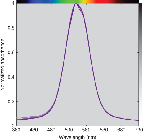
Figure 9.11 Normalized spectral absorbance of polystyrene plastic at varying thickness.
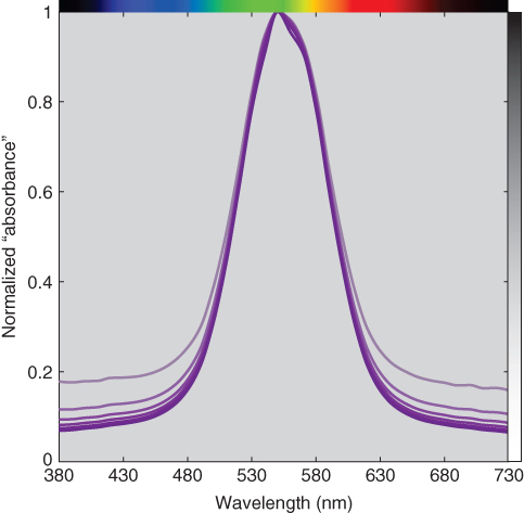
Figure 9.12 Normalized spectral “absorbance” of polystyrene plastic at varying thickness. First surface reflections were ignored in the calculation of absorbance.
Predicting thickness from transmittance measurements can be interpreted in terms of the generic approach to color modeling. The first step, discovering the linear model, was the Bouguer–Beer model using internal transmittance. The second step, discovering the relationship between the user controls and effective colorant amount, was assumed to be one‐to‐one. That is, ce = b. This assumption is often false when modeling opaque materials, described below.
A colorant's spectral properties can be used for identification. In this example all the plotted spectra are similar. However, decreases in thickness reduce the clarity of the spectral signature. In the same way that the base 10 logarithm of transmittance transformed an exponential relationship to a multiplicative relationship, the base 10 logarithm of absorbance transforms a multiplicative relationship to an additive relationship where the spectral signature is independent of thickness, shown in Figure 9.13. We recommend this practice when using visual methods for identification.
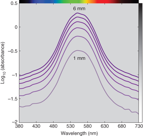
Figure 9.13 Base 10 logarithm of spectral absorbance of polystyrene plastic at varying thickness.
C. MODELING OPAQUE MATERIALS
Most colored materials are not transparent—they are either translucent or opaque, a result of internal scattering. An incident beam of light changes directions multiple times depending on the scattering properties of the colorants, their concentrations, their size and shape, how the colorants are dispersed within the material including orientation, and the thickness of the material. Determining the exact amount of reflection, absorption, and transmission is complex. Such calculations were first made in the field of astrophysics to understand how radiation is propagated through a foggy atmosphere (Schuster 1905). These calculations evolved tremendously throughout the twentieth century. See, for example, Rybicki and Lightman (2008). Beginning in the 1930s, Kubelka and Munk made a simplifying assumption that the light inside a scattering layer travels either up or down perpendicular to the plane of the sample nonpreferentially (Kubelka and Munk 1931; Kubelka 1948, 1954). This became known as the two‐flux model and enabled the modeling of opaque paints, plastics, and textiles, launching color‐formulation software in the middle of that century. Later developments included three‐ four‐ and many‐flux models, summarized by Völz (2001) and Klein (2010). Statistical approaches have also been derived, for example, Wang, Jacques, and Zheng (1995) and Rogers (2016).
Today's formulation systems use multiflux models, a term that implies traditional two‐flux modeling is not used, but little else because the specific mathematics are proprietary. Multiflux systems are used to model textiles, opaque and translucent paints and plastics, printing inks on a variety of substrates, multilayer materials, and to a limited extent, materials containing fluorescent and gonioapparent colorants. Because of the complexity of the mathematics, a thorough coverage of published models is beyond the scope of this book. However, the principles of using optical models to predict mixtures are the same irrespective of the model complexity, and we will use the two‐flux approach to model opaque paints and textiles. For good summaries of the use of Kubelka–Munk theory in color technology, see Kortüm (1969), Johnston (1973), Judd and Wyszecki (1975), Kuehni (1975), Allen (1980), Nobbs (1985), Park (1994), McDonald (1997), Nobbs (1997), Zhao and Berns (2009), and Hébert and Emmel (2015).
Kubelka and Munk considered a translucent colorant layer on top of an opaque background, shown in Figure 9.14. The colorant layer and background are in optical contact; that is, there is not a change in refractive index at this boundary. Within the colorant layer, both absorption, Kλ, and scattering, Sλ, occur and light flux travels in many directions. This was simplified to two light directions, up or down, also shown in Figure 9.14, which resulted in a pair of differential equations, one for each direction, shown in Eqs. (9.12) and (9.13)

Figure 9.14 Kubelka–Munk theory assumes that the light flux within a translucent absorbing and scattering layer having a thickness X on top of an opaque support with reflectance of Rg travels either downward (direction i) or upward (direction j).
Light in the downward, i, direction is weakened due to absorption and scattering, −(Kλ + Sλ)i, and strengthened by scattered light from the opposite direction, +Sλ, j. This also occurs in the upward direction. By convention, the downward direction is the negative direction, hence, −dx.
Solving the pair of differential equations (see Allen 1980; Haase and Meyer 1992; Hébert and Emmel 2015 for detailed descriptions of the calculus) results in Eqs. (9.14)–(9.17):
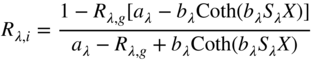
where internal reflectance, Rλ,i, is calculated from knowledge of the background reflectance, Rλ,g, the absorption, Kλ, and scattering, Sλ, properties of the colorant layer, and its thickness, X. Coth refers to the hyperbolic cotangent.
The key assumption in applying Kubelka–Munk theory is that the light within the colorant layer is completely diffuse, that is, the material is isotropic. As a result, Kubelka–Munk theory does not apply to most gonioapparent pigments or to colorant layers that change the degree of polarization of the incident light significantly. Kubelka–Munk theory also does not apply to fluorescent colorants though it is used as a starting point for more elaborate approaches (see Bonham 1986; Simon, Funk, and Laidlow 1994; McDonald 1997; Shakespeare and Shakespeare 2003). Finally, Kubelka–Munk theory applies to a single wavelength at a time, necessitating the use of a spectrophotometer. Theoretically, the geometry should be diffuse illumination and diffuse collection, which does not occur in any spectrophotometer. Nonetheless, Kubelka–Munk theory has been used successfully to model a number of coloration systems.
Kubelka–Munk theory is used to develop mixing laws for three types of samples, shown in Figure 9.15. The first is translucent materials where the general form of Kubelka–Munk theory as shown in Eq. (9.14) is used. Zhao and Berns (2009) have reviewed common approaches to modeling translucent materials using the general form. Equation (9.14) can be rearranged algebraically to facilitate calculating reflectance, transmittance, scattering, and absorption for a number of practical applications (Kubelka 1948). (Care should be taken in using these formulas because typographical errors occur in a number of references; we use Wyszecki and Stiles 1982 and Hébert and Emmel 2015.) Judd and Wyszecki (1975) provide several numerical examples.

Figure 9.15 Kubelka–Munk theory is most often applied to (a) translucent materials, (b) transparent colored layers on an opaque, scattering support, and (c) opaque materials.
The second type of sample is one in which a transparent colorant layer is in optical contact with an opaque, diffusely scattering support. As scattering of the colorant layer approaches zero, the general form reduces to Eq. (9.18)
This formula has been used to model photographic paper and continuous‐tone prints using thermal‐transfer technologies (Berns 1993b; Kang 1997).
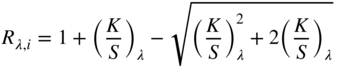
The third type of sample is opaque absorbing and scattering materials such as textiles, dyed paper, coatings, and plastics. At opacity, thickness is infinite, that is, an increase in thickness does not change reflectance, and the general form reduces to Eq. (9.19)
We will model opaque paints and textiles to illustrate the use of Kubelka–Munk theory.
Opaque Paints
Kubelka–Munk theory has been used to model opaque paint mixtures since the 1940s where each paint's absorption and scattering properties are used to define a linear model (Duncan 1940). This is shown in Eq. (9.20) for three colorants:

where ce denotes effective colorant amount and kλ and sλ are the absorption and scattering properties of a colorant at unit amount. This is often called two‐constant Kubelka–Munk theory since each colorant has two independent spectra.
For this example, ultramarine blue (PB 29), red iron oxide (PR 101), and titanium white (PW 6) matte artist acrylic dispersion paints were used. Ultramarine blue is nearly transparent while red iron oxide is nearly opaque. Mixtures were made of blue and white and red and white at percentage weight ratios of 80:20, 60:40, 40:60, and 20:80. Mixtures were also made of blue, red, and white at weight ratios of 50:50:0, 45:45:10, 30:30:40, 20:20:60, 10:10:80, and 5:5:90. Because weight ratios are used, there are only two unknowns when determining effective colorant amounts, shown in Eq. (9.21)

The mixtures were applied to contrast paper at a thickness of 0.006 in. (6 mil) using a drawdown bar. A drawdown of each paint at masstone (directly from the tube) was also made. The blue masstone drawdown was not opaque and the paint was reapplied on top of the first drawdown at 0.010 in. Example drawdowns are shown in Figure 9.16.
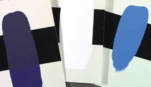
Figure 9.16 Drawdowns of ultramarine blue and titanium white at percentage weight ratios of 100:0, 0:100, and 60:40 (left to right).
An integrating sphere spectrophotometer with the specular component included was used to measure each drawdown in four locations against the white and the black areas of the contrast paper. In all cases, the measurements were within the precision of the spectrophotometer, verifying opacity. The average of the eight measurements was used in all subsequent calculations. The spectral data for each paint are plotted in Figure 9.17. Because of the high tinting strength of ultramarine blue, there is a large change in reflectance between the masstone (100:0) and the 80:20 tint. For all the tints, the maximum reflectance is bounded by white.

Figure 9.17 Spectral reflectance factor of ultramarine blue and red iron oxide tint ladders and masstones.
Kubelka–Munk theory predicts internal reflectance from colorant concentration and in similar fashion to modeling transparent materials, measured reflectance is converted to internal reflectance, in this case, using formulas first derived by Ryde (1931), Ryde and Cooper (1931), and later used by Saunderson (1942) when modeling pigmented plastics. The formulas can be generalized for both integrating sphere and bidirectional geometries, shown in Eqs. (9.22) and (9.23)


Constant K1 defines the amount of reflected collimated light at the boundary (i.e. surface of paint layer) and is calculated using the Fresnel formulas. Inside the paint layer, light is scattered equally in all directions and as a result, the light striking the boundary in the upward direction has a range of incident angles between 0° and 90° relative to the surface normal. Constant K2 defines the integration of all the light reflecting at the boundary over this range of angles except the collimated angle. If the incident light is along the normal and the refractive index of the paint layer is 1.5, then K1 = 0.04 and K2 = 0.6 (Orchard 1969). Constant Kinstrument is the proportion of the collimated light reflecting from the surface that is included in the reflectance measurement. For an integrating sphere spectrophotometer with the specular component included, Kinstrument = 1. When the geometry is bidirectional, Kinstrument = 0. For integrating spheres with the specular component excluded, Kinstrument depends on the material's gloss and the integrating sphere design, discussed in Chapter 6. The conversion from measured to internal reflectance and the reverse is known as the Saunderson correction.
The constants K1 and K2, by definition, are wavelength dependent since their values are based on the paint layer's refractive index, also wavelength dependent. When using Kubelka–Munk theory to model opaque materials, wavelength dependency is ignored. Furthermore, rather than define the values based on spectrophotometer geometry and average refractive index, they are determined empirically as we describe below. Optimizing the Saunderson constants has the effect of improving the linearity between measured weight and ce.
Predicting the spectral reflectance of a paint mixture requires K1, K2, Kinstrument, and each colorant's unit kλ and sλ. We use a two‐step approach to determine these optical parameters (described in detail below). First, reasonable values for the Saunderson correction constants are defined and unit kλ and sλ are calculated directly. Second, nonlinear optimization is used where the first‐step data become starting values. For both steps it is assumed that ce equals measured weight.
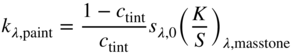
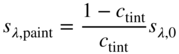
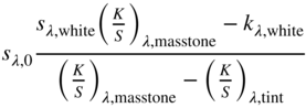
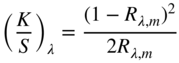
Evaluating the minimum reflectance factor of all the measured samples, K1 was defined as 0.03 and K2 was defined as 0.5, the midpoint between the theoretical value of 0.6 and 0.4 as used by Saunderson (1942). Kinstrument was defined as 1.0. When the samples are opaque, it is common to define sλ,white = 1 and kλ,white = (K/S)λ,white where the transformation between Rλ,i and (K/S)λ is shown in Eq. (9.24)

The spectra for the masstone (100:0), 20:80 tint, and white (0:100) were used to calculate kλ and sλ, the formulas shown in Eqs. (9.25)–(9.27) (Berns and Mohammadi 2007a; Zhao and Berns 2009)
These were used as starting values for a nonlinear optimization estimating K1, K2, and kλ and sλ for blue and red where RMS spectral reflectance error was minimized. We prefer minimizing reflectance error rather than K/S to reduce the influence of dark colors such as masstones on estimating k and s. Nonlinear optimization requires reasonable starting values in order to converge to the minimum error, hence the need for the first step. The optimized K1 and K2 were 0.03 and 0.74, respectively. The unit data are plotted in Figure 9.18. As expected, the scattering of blue is nearly zero, whereas the scattering for red is quite large. There is an increase in k and s for both paints between 380 and 400 nm. This is an artifact of using a white paint with strong absorption in this region. Data for red at 450 nm are given in Table 9.2.

Figure 9.18 Unit k (blue line) and s (red line) for (a) ultramarine blue and (b) red iron oxide. Note the differences in the y‐axis scales.
Table 9.2 Numerical data for red iron oxide at 450 nm for K1 = 0.03 and K2 = 0.74.
| Sample | Rm | Ri | K/S |
| 100:0 (masstone) | 0.0438 | 0.0585 | 7.5766 |
| 80:20 | 0.0776 | 0.1694 | 2.0361 |
| 60:40 | 0.1141 | 0.2697 | 0.9888 |
| 40:60 | 0.1804 | 0.4143 | 0.4141 |
| 20:80 | 0.2749 | 0.5644 | 0.1681 |
| 0:100 (white) | 0.8893 | 0.9673 | 0.0006 |
The model was evaluated several ways. Another optimization was performed to estimate ce for each of the tints and masstones where RMS spectral reflectance error was minimized, the spectral results plotted in Figure 9.19. This is known as spectral matching, sometimes used in color formulation. This obviates assuming that ce equals measured weight. The spectral similarity is a measure of scalability, which was reasonable for these paints. The effective and measured ratios were compared and differences were within the precision of the scale, that is, there was a linear relationship. This result is important because linearity was assumed when the optical parameters were estimated. Second, the ce were estimated for the blue, red, and white mixtures where RMS spectral reflectance error was minimized, the spectral results plotted in Figure 9.20. Spectral accuracy was similar to the accuracy of the estimated tints. The effective and measured ratios were compared, the results plotted in Figure 9.21. There was a lack of linearity that exceeded scale imprecision, particularly for the mixture without white where the blue:red:white effective colorant amount ratio was 53:47:0 instead of the weighed ratio of 50:50:0. This discrepancy is typical for mixtures without white.

Figure 9.19 Measured (thick lines) and estimated (thin lines) spectral reflectance factor of ultramarine blue and red iron oxide tint ladders and masstones using two‐constant Kubelka–Munk theory.

Figure 9.20 Measured (thick lines) and estimated (thin lines) spectral reflectance factor of 6 mixtures containing ultramarine blue, red iron oxide, and titanium white using two‐constant Kubelka–Munk theory.
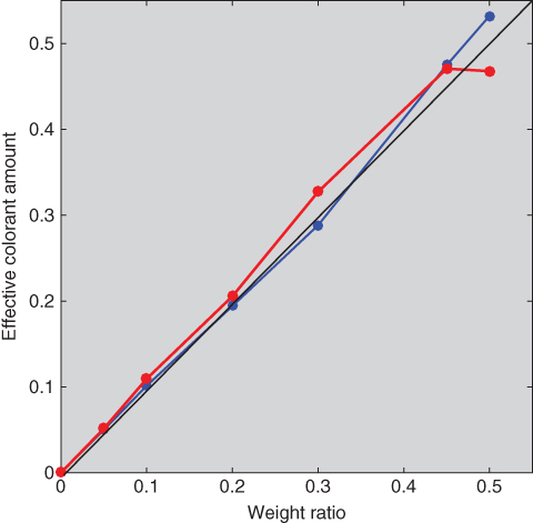
Figure 9.21 Relationship between actual weight and ce of ultramarine blue (blue line) and red iron oxide (red line) for mixtures using two‐constant Kubelka–Munk theory.
Two‐constant Kubelka–Munk theory can be simplified for cases where scattering is dominated by white such as pastels (Billmeyer and Abrams 1973; Berns and Mohammadi 2007b). The Duncan formula, shown in Eq. (9.20), changes to Eq. (9.28), which can be rewritten as in Eqs. (9.29) and (9.30)
This simplification is known as single‐constant Kubelka–Munk theory.
Unit (k/s)λ spectra were estimated for blue and red using the tints minimizing RMS spectral reflectance error. The 20:80 tint was used to calculate starting values where (k/s)λ = (K/S)λ/0.2. Then, ce were estimated, also minimizing RMS spectral reflectance error. The predicted spectra are shown in Figure 9.22 and the effective and measured ratios are shown in Figure 9.23. The results for blue are similar to the two‐constant model because ultramarine blue is a weak scatterer. For red, the single‐constant simplification resulted in poor spectral accuracy and nonlinearity between weight and effective colorant amount because red oxide is a strong scatterer.
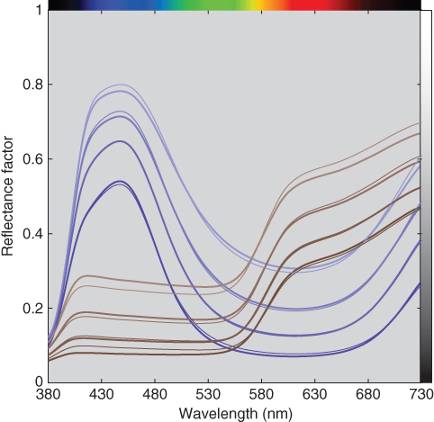
Figure 9.22 Measured (thick lines) and estimated (thin lines) spectral reflectance factor of ultramarine blue and red iron oxide tint ladders using single‐constant Kubelka–Munk theory.
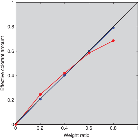
Figure 9.23 Relationship between actual weight and ce of ultramarine blue (blue line) and red iron oxide (red line) tint ladders using single‐constant Kubelka–Munk theory.
One limitation of the single‐constant approach is that mixtures without white are undefined when cwhite = 0. Abed and Berns (2017) modified single‐constant Kubelka–Munk theory to overcome this limitation by assuming that the scattering of the nonwhite paint is a portion of the white's scattering. That is, sλ,paint becomes ppaintsλ,white where p is an impurity index where a nonwhite paint's scattering reduces the purity of the white. Rather than associating the impurity index with the white's unit scattering coefficient, it is associated with concentration, ce,paintppaint. Equation (9.29) becomes Eq. (9.31)

The impurity index, p, and (k/s)λ were estimated for blue and red using the tints and masstones where RMS spectral reflectance error was minimized. The optimized unit (k/s)λ and p = 0.5 were used as starting values. The impurity indices for blue and red were 0.006 and 0.386, respectively. Then, ce were estimated, also minimizing RMS spectral reflectance error. The predicted spectra are shown in Figure 9.24 and the effective and measured ratios are shown in Figure 9.25. The spectral estimation accuracy was similar to the single‐constant predictions. However, the relationships between weight and effective colorant amount had similar accuracy to the two‐constant predictions, verifying the effectiveness of the impurity index.
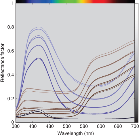
Figure 9.24 Measured (thick lines) and estimated (thin lines) spectral reflectance factor of ultramarine blue and red iron oxide tint ladders using single‐constant Kubelka–Munk theory with an impurity index.
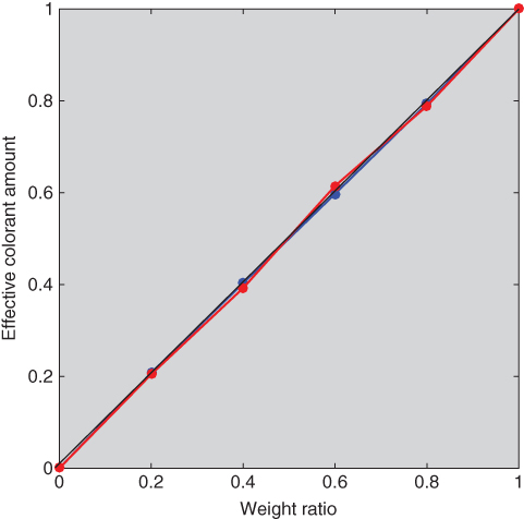
Figure 9.25 Relationship between actual weight and ce of ultramarine blue (blue line) and red iron oxide (red line) tint ladders using single‐constant Kubelka–Munk theory with an impurity index.
ce were optimized separately from the unit spectra and Saunderson constants for all three models. We have found that for the two‐constant form of Kubelka–Munk theory, convergence is difficult as well as the results not improving significantly when all the optical parameters are optimized simultaneously. The same approach was used for the single‐constant models for simplicity. Simultaneous optimization is used when modeling opaque textiles, described below.
Opaque Textiles
Textiles are opaque because the substrate scatters incident light, whether in fiber, yarn, or woven form. In most cases, the amount of scattering is large compared with scattering by colorants. This is also true for colored paper. When colorant scattering is negligible, single‐constant Kubelka–Munk theory can be used, shown in Eqs. (9.32)–(9.35). The Saunderson correction is not required because the textile or paper fibers are immersed in air

As an example, polyester fabric was cold pad‐batch dyed using red, yellow, and blue disperse dyes. Tint ladders were made where the fabric was dyed at concentrations of 0.0, 0.1, 0.5, 1.0, 2.0, and 5.0 grams per liter (g/l). Null concentration dyeings are called blank dyeings, important because the dyeing process can change the optical properties of the substrate. Fabrics were also dyed using two and three colorant combinations. Each dyed fabric was folded in half to achieve opacity and four measurements were taken, one at each rotation in four different locations, using an integrating sphere spectrophotometer with the specular component included. The four measurements were averaged and the spectra are shown in Figure 9.26. These spectra were transformed to K/S using Eq. (9.32), the results shown in Figure 9.27. Reflectance factor and K/S are inversely related, similar to the paint spectra shown above.
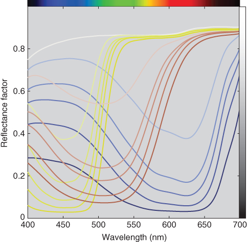
Figure 9.26 Spectral reflectance factor of polyester tints and blank‐dyed fabric.

Figure 9.27 K/S spectra of polyester tints and blank‐dyed fabric.
Equation (9.36) was used to normalize the spectra in order to evaluate scalability, the results shown in Figure 9.28


Figure 9.28 Normalized (K/S) spectra of polyester tints.
Scalability was reasonable for the three colorants between 0.0 and 2.0 g/l. The 5.0 g/l blue and yellow samples had spectra with wider bandwidth, indicating that single‐constant theory is inadequate to model this coloration system at high concentrations. The 5.0 g/l samples for all three colorants were excluded limiting color matching to 2.0 g/l. The 0.5 g/l red sample also had a wider bandwidth, a result of poor dyeing uniformity of the fabric. Excluding the 0.5 g/l red sample did not change the results and was retained for consistency.
Unit (k/s)λ were calculated using the 0.0 and 1.0 g/l samples, the formula shown in Eq. (9.37)
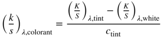
These unit data and actual concentrations were used as starting values in an optimization that predicted (k/s)λ and ce for all of the samples for each colorant where RMS spectral reflectance error was minimized. The resulting (k/s)λ for red, yellow, and blue are shown in Figure 9.29. Integrating (k/s)λ as a function of wavelength is sometimes used as a measure of tinting strength and depth of shade, useful when comparing batches of colorants that are priced according to their strength or depth (Smith 1997). For this example, the tinting strengths of red, yellow, and blue were 20.0, 34.4, and 35.3, respectively.
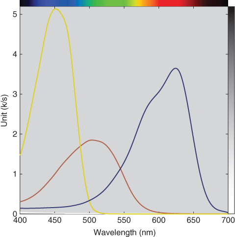
Figure 9.29 Unit (k/s)λ of red, yellow, and blue colorants.
The optimization results in estimated reflectance spectra and ce. Equations (9.38) and (9.35) are used to calculate estimated spectral reflectance
Comparison of the estimated and measured reflectance spectra was used to evaluate scalability in addition to Figure 9.28, shown in Figure 9.30. The blue sample matches were excellent; the yellow matches were reasonable; and the red matches were poor at long wavelengths. The relationship between concentration and ce is shown in Figure 9.31. None of the colorants exhibited monotonicity, a result of poor process control. Exhaust dyeing would improve these results. Typically, ce reduces as concentration increases because available dye sites are depleting. This was tested for the red colorant by adding back the 5.0 g/l tint and repeating the optimization, the results shown in Figure 9.32. (Recall that the red colorant was scalable at this high concentration, seen in Figure 9.28.) The reduction in effective colorant amount is evident. The data plotted in Figure 9.32 would be used to define the relationship between user controls, concentration, and ce, the second step in the generic approach to color modeling.

Figure 9.30 Measured (thick lines) and estimated (thin lines) spectral reflectance factor of the red, yellow, and blue tints using single‐constant Kubelka–Munk theory.
Figure 9.31 Relationships between concentration and ce for the red, yellow, and blue tints.
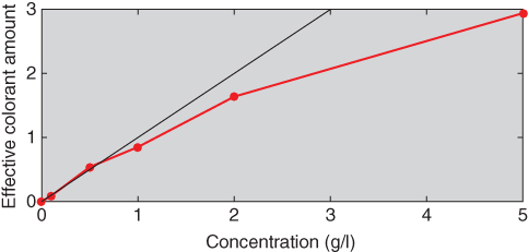
Figure 9.32 Relationship between concentration and ce for red tints ranging between 0.0 and 5.0 g/l.
Nine two‐colorant dyeings were made for all combinations of 0.5, 1.0, and 2.0 g/l. Two three‐colorant dyeings were also performed at concentrations of 0.1 and 1.0 g/l for each colorant. The (k/s)λ for each of the colorants were used to estimate ce, minimizing RMS spectral reflectance error. The spectral fits are shown in Figure 9.33 for the 11 samples. The results were reasonable for mixtures with blue and yellow and blue and red. The results for mixtures with red and yellow were poor at long wavelengths.
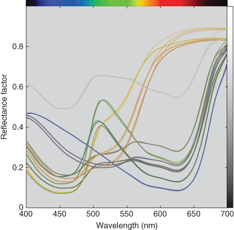
Figure 9.33 Measured (thick lines) and estimated (thin lines) spectral reflectance factor of 2 and 3 colorant mixtures using single‐constant Kubelka–Munk theory.
The relationship between concentration and ce for all of the samples is shown in Figure 9.34. We expected modest variability about the tint lines. This did not occur. Instead there was large variability as well as an increase in the range of values with an increase in concentration. It is unclear whether this large variability is attributed mainly to poor process control or limitations in Kubelka–Munk theory. If the former, the process needs to be improved or replaced. If the latter, then a three‐dimensional lookup table may be warranted.
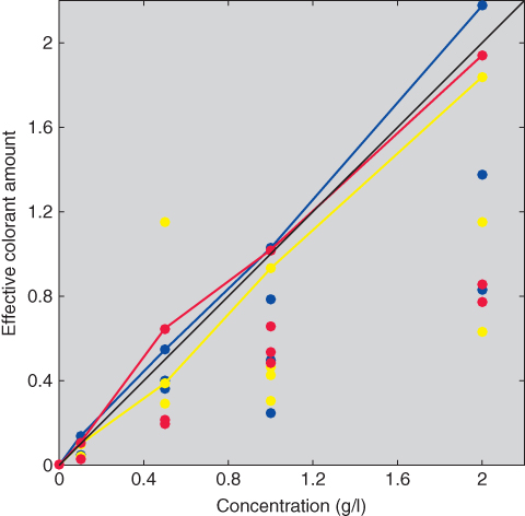
Figure 9.34 Relationships between concentration and ce for all the samples.
D. MODELING GONIOAPPARENT MATERIALS
Gonioapparent materials change their appearance with changes in illuminating and viewing geometries, as described in Chapter . Gonioapparent materials include metallic flakes, pearlescent pigments, interference pigments, and diffraction pigments. These are used in addition to or in place of conventional absorbing and scattering colorants. Automotive coatings, printing inks, and cosmetics are examples of these materials. Models are used to predict spectral reflectance at geometries used by multiangle spectrophotometers and can be generalized to predict bidirectional reflectance distribution functions (BRDFs), required for computer graphics rendering. Researchers in computer graphics have been active in modeling many kinds of materials since the 1960s, summarized by Dorsey, Rushmeier, and Sillion (2008) and Montes and Ureña (2012). Models specific to coatings include Germer and Nadal (2001), Ďurikovič and Ágošton (2007), and Ferrero et al. (2016). Examples of using BRDF measurements for product design include Ďurikovič and Ágošton (2007), Kim and Lee (2011), Shimizu and Meyer (2015), and Musbach (2016). A simulation of an automotive coating containing aluminum flake is shown in Figure 9.35. Models that predict the optical behavior of gonioapparent materials are very complex and beyond the scope of this book. We suggest the books by Völz (2001), Klein (2010), and Kettler et al. (2016) as starting points.

Figure 9.35 Simulation of aluminum flake in a lacquer containing red dye, over gray primer (Musbach 2016).
E. COLOR‐FORMULATION SOFTWARE
Color‐formulation software, also known as color‐matching software, is designed to aid a colorist in selecting colorants and determining their concentrations in order to match a color standard. The standard can be a physical sample, spectral data, or a colorimetric specification. Formulation software has three main components. The first is a database of the optical properties of the coloration materials. The second is the algorithms that select the colorants and predict a formulation (recipe). The third is the algorithms that correct the initial recipe when the match is not within tolerance, also known as batch correction.
Spectral‐based algorithms require a spectrophotometer with high precision and accuracy. If numerical data are used to define the standard, intrainstrument and interinstrument reproducibility must also be excellent, considered in detail in Chapter 6.
The success of formulation software depends on a consistent and repeatable coloration process. The phrase “garbage in, garbage out” comes to mind. This is evaluated both in the color laboratory and in manufacturing. If the same recipe is used to make 10 samples, will the same color result? If the process variability and manufacturing tolerance are similar, producing an acceptable batch will only occur by chance. Changing software will not improve the odds. It is absolutely essential to evaluate the process and make improvements if repeatability is poor.
The next step is to prepare samples that will be used to create the optical database. Different software requires different kinds and numbers of samples. Replicates are important in case there is a process error. A weighing error during database development will affect formulation accuracy.
Many matching algorithms are possible. For a spectral‐based standard, the best formulation results in a spectral match. This eliminates metamerism. When a spectral match is not achievable, the least metameric formulation is the best. For a colorimetric standard, the best formulation is the most color constant. Indices of metamerism and color inconstancy are described in Chapter . These are used to rank order potential formulations. We have not listed cost in our definition of best. Any future issues with metamerism or color inconstancy will negate initial cost savings. For example, a commercial color order system was produced for a period of time where samples were replenished that had the lowest cost. The spectra from a constant‐hue page are shown in Figure 9.36. Ideally, all the spectra should have similar shape so that the samples have similar color constancy. There are two types of spectra. Spectra having peak wavelengths at 560 nm were formulated for lowest cost. A visualization of the samples illuminated by illuminants D65 and A is shown in Figure 9.37. The samples formulated for least cost have very different color constancy where they become greenish under illuminant A. This difference in color constancy occurs for many illuminants. As a consequence, viewing this page under nonstandard lighting greatly reduces the utility of a physical color order system.
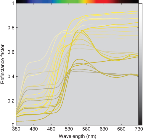
Figure 9.36 Spectral reflectance factor of samples at constant hue from a physical color order system.

Figure 9.37 Visualization of the spectra shown in Figure 9.36 illuminated by (a) CIE illuminant D65 and (b) CIE illuminant A, viewed by the 1931 CIE standard observer.
The relationships between concentration and spectral reflectance and between concentration and colorimetry are nonlinear and accordingly, nonlinear optimization algorithms are required. These are constrained optimizations where concentration cannot be negative and in the case of paint, the sum of concentrations equals unity. Nonlinear optimization has the disadvantage of sometimes converging on a local minimum, resulting in a recipe that is correct, but not its best. This limitation is minimized by having reasonable starting values. For spectral algorithms, least squares linear regression can be used minimizing RMS K/S error (McGinnis 1967; Walowit, McCarthy, and Berns 1988). For colorimetric algorithms, pseudo‐tristimulus values are calculated using K/S or weighted K/S in place of reflectance where the weighting improves linearity between concentration and pseudo‐tristimulus values (Allen 1966, 1974, 1980). The pseudo‐tristimulus values are used as additive primaries and concentration is estimated in the same manner as calculating RGB for a specific XYZ. See Berns (1997, 2000) for more details.
The second aspect of the matching algorithm is choosing the best colorants. Process variability is added to least metameric or least color inconstant when defining “best.” There may be two formulations with similar color inconstancy. The formulation that leads to the smallest colorimetric variability is preferred. The optical model can be used to calculate the variability.
A third aspect is selecting the colorants to evaluate. Degrees of freedom come into play. Colorants were defined as ratios in the paint example and the white concentration was the remainder. If the formulation has four colorants, for example, three chromatic colorants and white, there are three degrees of freedom. There is always one less degree of freedom than the total number of colorants. When dispensing color concentrates into a base paint, such as retail paint and hardware stores, each concentrate has a single degree of freedom and the total degrees of freedom equal the number of concentrates. This is also true when dyeing textiles. Least‐squares estimates have one degree of freedom less than the number of data points. For a wavelength range of 380–730 nm in 10 nm increments, there are (36 − 1) degrees of freedom. In theory, the maximum number of colorants used in a formulation when spectral matching equals the number of degrees of freedom. It would seem that adding colorants will reduce metamerism—each additional colorant enables a match at an additional wavelength. This does not occur because absorption is across many wavelengths. Adding colorants rarely reduces metamerism. A colorimetric specification has three degrees of freedom, for example, XYZ or L*a*b*. The degrees of freedom in a coloration system cannot exceed three.
Practically, the number of chromatic colorants in a formulation should not exceed four, that is, four degrees of freedom. Every combination of one, two, three, and four colorants should be evaluated. The number of combinations is calculated using Eq. (9.39):
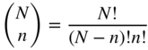
where N defines the total number of colorants and n defines the number of colorants in a formulation. For 10 colorants, there are 10, 45, 120, and 210 one, two, three, and four colorant combinations, respectively. Equation (9.39) was enumerated for up to 25 colorants, shown in Figure 9.38. The total number of formulations for 25 colorants is 15 275. Limiting the formulation to three chromatic colorants reduces this number to 2625.
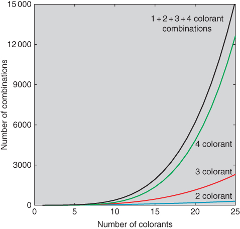
Figure 9.38 Number of combinations as a function of the total number of colorants, based on enumerating Eq. (9.39).
The approach we take when formulating is to test every combination. When the standard has spectral data, least squares linear regression minimizing K/S RMS error is used to obtain starting values. Then spectral reflectance RMS error is minimized. Finally, ΔE00 is minimized for a primary illuminant. Equation (8.2) is used as a special index of metamerism or Eqs. (8.17) and (8.21) are used as a general index of metamerism. The effect of process variability is calculated by adding normally distributed random variability to each colorant in the formulation. Concentration defines the mean and the standard deviation is based on the process variability. The colorimetric data for the actual and perturbed formulations are compared and CIEDE2000 calculated for the primary illuminant. This is repeated 100 times. The average ΔE00 between the formulation and the 100 perturbations defines the process variability. The data are sorted first by metamerism and secondly by process variability and the best formulation selected. The approach we take when formulating to a colorimetric standard is to minimize ΔE00 and discard formulations that do not achieve a colorimetric match. The data are sorted first by color constancy and secondly by process variability.
For example, two‐constant Kubelka–Munk theory was used to formulate the 16 gray metamers described in Chapter . Three were selected, their reflectance spectra shown in Figure 9.39 and their recipes and indices listed in Table 9.3. The first formulation is the closest spectral match. It is dominated by bone black and titanium white. The second formulation also contains bone black. However, its concentration is about half the amount of the first formulation, and as a consequence, the chromatic colorants have more of an influence on its spectral characteristics. The third formulation does not contain black but contains appreciable cobalt blue. This results in the large spectral mismatch at long wavelengths. All of the indices are correlated with each other and with the magnitude of spectral mismatch, quantified by reflectance RMS difference. Process variability was assumed to result from weighing imprecision. For formulations summing to unity, the standard deviation was defined as 0.025. This uncertainty occurs for all four paints and is independent of weight ratio. This translates to ±0.006c. In this example, process variability correlated with the degree of metamerism. Clearly, Formulation 1 is the best formulation.
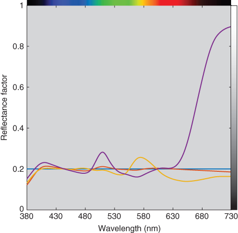
Figure 9.39 Spectral reflectance factor of standard (blue line), metamer 1 (red line), metamer 2 (orange line), and metamer 3 (purple line).
Table 9.3 Colorant amounts, metamerism indices, and process variability of three of the 16 metamers formulated for Chapter .
| Formulation 1 | Formulation 2 | Formulation 3 | |
| Colorant 1 | Arylide yellow | Pyrrole orange | Arylide yellow |
| Colorant 2 | Quinacridone magenta | Phthalocyanine green | Cobalt blue |
| Colorant 3 | Bone black | Bone black | Quinacridone magenta |
| ce,1 | 0.03 | 0.16 | 0.11 |
| ce,2 | 0.03 | 0.12 | 0.44 |
| ce,3 | 0.59 | 0.33 | 0.11 |
| cwhite | 0.35 | 0.39 | 0.33 |
| Reflectance RMS difference | 0.016 | 0.034 | 0.301 |
| Special metameric index, ΔE00 | 0.1 | 3.5 | 5.4 |
| General metameric index, Viggiano | 0.0014 | 0.0058 | 0.0080 |
| Process variability for primary illuminant, ΔE00 | 0.6 | 2.0 | 3.5 |
The third component, when required, is adjusting the initial formulation to more closely match the standard. Kubelka–Munk and possibly other optical models have limited accuracy, and as a result, either a second sample needs to be made in the laboratory or the production process adjusted. The measured spectral reflectance of the first sample is treated as a new standard and a formulation is determined. The differences between the initial and reformulated concentrations are used to create correction factors that adjust the relationship between weight and ce. See McDonald (1997), Nobbs (1997), and Berns (2000) for more details. The adjustments are specific to the set of colorants. These corrections become part of the optical database and are used in future formulations when using the same colorants with similar concentrations.
Over time, a database is developed consisting of concentrations and colorimetric data. This is a multidimensional lookup table. The model can be replaced with the table and linear interpolation used to calculate a recipe for a specific color. The database can also be used as training data to create a neural network or other learning‐based algorithm. The latter technique might lead to higher accuracy when the database is sparsely populated. These database approaches are very useful when an optical model cannot be developed with sufficient accuracy.
F. SUMMARY
Optical models of colored materials are used for both product development and color formulation. Modeling transparent materials, paints, and plastics requires calculating either internal transmittance or reflectance. The Fresnel and Saunderson formulas are used. Transparent materials such as glass and colorants dissolved in a solvent are modeled using the Bouguer–Beer law where transmittance is predicted from path length and concentration. Scattering materials such as coatings and textiles are modeled based on radiative transfer theory, pioneered by Shuster at the beginning of the twentieth century. Models used for predicting reflectance from colorant concentration simplify radiative transfer theory by assuming that light (flux) travels in only a specific number of directions. Examples include two‐, three‐, four‐, many‐, and multi‐flux models. The two‐flux model derived by Kubelka and Munk has been used extensively to model opaque materials and led to the development of colorant formulation software during the mid‐twentieth century. The success of this software depends on process repeatability both in the laboratory and in production. Samples are prepared at various concentrations and when translucent, also at various thicknesses. They are measured with a spectrophotometer and used to develop an optical database. Formulations are predicted that match a standard using the colorants stored in the database. When the standard is spectral, the best match is the least metameric. When the standard is colorimetric, the best match is the most color constant. Formulations can also be evaluated for process variability and those leading to the smallest variability in total color difference are preferable. Selecting the best formulation is the most important feature of the software, particularly when the number of colorants in the database is large. Sometimes, materials, especially those containing gonioapparent pigments, cannot be modeled with sufficient accuracy and table lookup and learning‐based algorithms are used.