
3.5. Concluding Remarks
This chapter has detailed the algorithmic and convergence property of the EM algorithm. The standard EM has also been extended to a more general form called doubly-stochastic EM. A number of numerical examples were given to explain the algorithm's operation. The following summarizes the EM algorithm:
EM offers an option of "soft" classification.
EM offers a "soft pruning" mechanism. It is important because features with low probability should not be allowed to unduly influence the training of class parameters.
EM naturally accommodates model-based clustering formulation.
EM allows incorporation of prior information.
EM training algorithm yields probabilistic parameters that are instrumental for media fusion. For linear-media fusion, EM plays a role in training the weights on the fusion layer. This will be elaborated on in subsequent chapters.
Problems
Assume that you are given a set of one-dimensional data X = {0, 1, 2, 3, 4, 3, 4, 5}. Find two cluster centers using
the K-means algorithm
the EM algorithm
You may assume that the initial cluster centers are 0 and 5.
Compute the solutions of the single-cluster partial-data problem in Example 2 of Figure 3.3 with the following initial conditions:
In each iteration of the EM algorithm, the maximum-likelihood estimates of an M-center GMM are given by
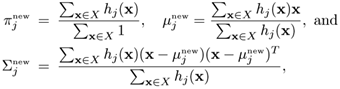
where
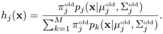
X is the set of observed samples.
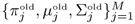 are the maximum likelihood estimates of the last EM iteration, and
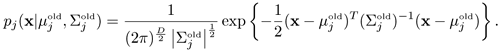
State the condition in which the EM algorithm reduces to the K-means algorithm.
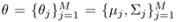
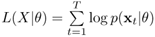
You are given a set X = {x1,..., xT} of T unlabeled samples drawn independently from a population whose density function is approximated by a GMM of the form
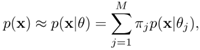
where
 are the means and covariance matrices of the component densities
  . Assume that πj are known, θj and θi(i ≠ j) are functionally independent, and xt are statistically independent.
Show that the log-likelihood function is
Hence, show that if
 are known, the maximum-likelihood estimate
  , i = 1;...;M are given by
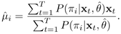
Hence, state the conditions where the equation in Problem 4c reduces to the K-means algorithm. State also the condition where the K-means algorithm and the equation in Problem 4c give similar solutions.
Based on the normal distribution
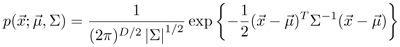
in D-dimensions, show that the mean vector and covariance matrix that maximize the log-likelihood function

are, respectively, given by
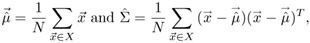
where X is a set of samples drawn from the population with distribution
 , N is the number of samples in X, and T denotes matrix transpose.
Hint: Use the derivatives
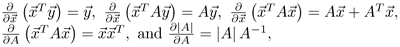
where A is a symmetric matrix.
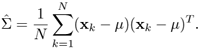
Let p(x|∑) ≡ N(μ, ∑) be a D-dimensional Gaussian density function with mean vector μ, and covariance matrix ∑. Show that if μ, is known and ∑ is unknown, the maximum-likelihood estimate for ∑ is given by
LBF-Type EM Methods: The fitness criterion for an RBF-type EM is determined by the closeness of a cluster member to a designated centroid of the cluster. As to its LBF-type counterpart, the fitness criterion hinges on the closeness of a subset of data to a linear plane (more exactly, hyperplane). In an exact fit, an ideal hyperplane is prescribed by a system of linear equations: Axt + b = 0, where xt is a data point on the plane. When the data are approximated by the hyperplane, then the following fitness function

should approach zero. Sometimes, the data distribution can be better represented by more than one hyperplane. In a multiplane model, the data can be effectively represented by say N hyperplanes, which may be derived by minimizing the following LBF fitness function:
Equation 3.5.1

where h(i)(xt) is the membership probability satisfying ∑j h(j)(xt) = 1. If h(j)(xt) implements a hard-decision scheme, then h(j)(xt) = 1 for the cluster members only, otherwise h(j)(xt) = 0.
Compare the LBF-based formulation in Eq. 3.5.1 with the RBF-based formulation in Eq. 3.3.13.
Modify an RBF-based EM Matlab code so that it may be applicable to either RBF-based or LBF-based representation.
The following is a useful optimization formulation for the derivation of many EM algorithms. Given N known positive values un, where n = 1, . . . , N. The problem is to determine the unknown parameters wn to maximize the criterion function
Equation 3.5.2

under the constraints wn > 0 and
 .
.Provide a mathematical proof that the optimal parameters have a closed-form solution:
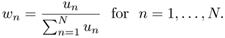
Hints: refer to Eqs. 3.2.23 through 3.2.26.
As an application example of the EM formulation in Eq. 3.2.10, what are the parameters corresponding to the known positive values un and the unknown positive values wn. Hence, provide a physical meaning of the criterion function in Eq. 3.5.2.
As a numerical example of the preceding problem, given u1 = 3, u2 = 4, and u3 = 5, and denote x = u1, y = u2, and 1 − x − y = u3, the criterion function can then be expressed as

Write a simple Matlab program to plot the criterion function over the admissible space 0 < x, 0 < y, and x + y < 1 (verify this range!).
Show numerically that the maximum value occurs at
 and
and  .
.
Suppose that someone is going to train a GMM by the EM algorithm. Let T denote the number of patterns, M the number of mixtures, and D the feature dimension. Show that the orders of computational complexity (in terms of multiplications) for each epoch in the E-step is O(TMD + TM) and that in the M-step is O(2TMD).
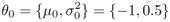
Assume that you are given the following observed data distribution:

Assume also that when EM begins, n = 0 and
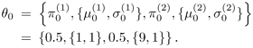
Derive

In a similar manner, derive
 .
.Substituting X = {1, 2, 4, 8, 9} into your derivation to obtain the corresponding membership values.
Substitute the derived membership values into Eqs. 3.2.17 through 3.2.19, and compute the values of the new parameters θ1.
To do more iterations, one can continue the algorithm by computing Q(θ|θi), which can again be substituted into Eqs. 3.2.17 through 3.2.19 to obtain θ2. Perform the iterative process until it converges.
It is difficult to provide any definitive assurance on the convergence of the EM algorithm to a global optimal solution. This is especially true when the data vector space has a very high dimension. Fortunately, for many inherently offline applications, there is no pressure to produce results in realtime speed. For such applications, the adoption of a user interface to pinpoint a reasonable initial estimate could prove helpful. To facilitate a visualization-based user interface, it is important to project from the original t-space (via a discriminant axis) to a two-dimensional (or three-dimensional) x-space [367, 370] (see Figure 2.7). Create a Matlab program to execute the following steps:
Project the data set onto a reduced-dimensional x-space, via say PCA.
Select initial cluster centers in the x-space by user's pinpoint. Based on the user-pinpointed membership, perform the EM algorithm in the x-space.
Calculate the values of AIC and MDL to select the number of clusters (see the next problem).
Trace the membership information back to the t-space, and use the membership function as the initial condition and further fine-tune the GMM clustering by the EM algorithm in the t-space.
Given a set of observed data X, develop Matlab code so that the estimated probability density p(x) can be represented in terms of a set of means and variances.
Use Matlab to create a three-component Gaussian mixture distribution with different means and variances for each Gaussian component. Ensure that there is some overlap among the distributions.
Use 2-mean, 3-mean, and K-mean algorithms to cluster the data.
Compute the likelihood of the true parameters (means and variances that define the three Gaussian components) and the likelihood of your estimates. Which of your estimates is closest to the true distribution in the maximum-likelihood sense?
Compute the symmetric divergence between the true Gaussian distributions and your estimates. Hint: Given two Gaussian distributions Λj and Λk with mean vectors μj and μk and covariance matrices ∑j and ∑k, their symmetric divergence is
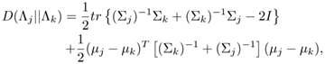
where I is an identity matrix.
Repeat (a), (b), and (c) with the EM clustering algorithm.
Use Matlab to create a mixture density function with three Gaussian component densities. The prior probabilities should be as follows:
Use 2-mean, 3-mean, and 4-mean VQ algorithms. Compute the likelihood between the data distribution and your estimate. Repeat the problem with the EM clustering algorithm.