5.4. The Back-Propagation Algorithms

The most prominent algorithm for training multi-layer networks is the so-called back-propagation (BP) algorithm. The algorithm, independently proposed by Wer-bos [377], Parker [269], and Rumelhart et al. [326], offers an efficient computational speedup for training multi-layer networks. The objective is to train the weights w_ji(l) so as to minimize the mean-squared error E in Eq. 5.3.1. The basic gradient-type learning formula is

Equation 5.4.1

with the n-th training pattern, a⁽ⁿ⁾(0), and its corresponding teacher t⁽ⁿ⁾, n = 1, 2,. . ., N, presented. The derivation of the BP algorithm follows a chain-rule technique:

Equation 5.4.2

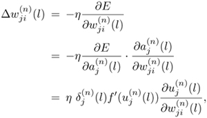
where the error signal is defined as

The error signal can be obtained recursively by back-propagation:

• Initial (Top) Layer. For the recursion, the initial value (of the top layer), , can be obtained easily as follows:

  Equation 5.4.3

  

  
  

  For an energy function other than the LSE, the initial condition can be similarly derived.

• Recursive Formula. The general BP recursive formula for the error signal, , can be derived as follows:

  

  
  

Equation 5.4.4

in the sequence of l = L — 1, . . . , 1. From Eq. 5.3.3, it follows that

Equation 5.4.5

The recursive formula is the key to back-propagation learning. It allows the error signal of a lower layer to be computed as a linear combination of the error signals of the upper layer . In this manner, the error signals are back propagated through all of the layers from the top down. This also implies that the influences from an upper to a lower layer (and vice versa) can only be effected via the error signals of the intermediate layers.

The general training algorithm described before is applicable to two types of prominent multi-layer networks: multi-layer LBF networks and multi-layer RBF networks.

5.4.1. BP Algorithm for Multi-Layer LBF Networks

A multi-layer linear basis function (LBF) network is characterized by the following equations:

Equation 5.4.6

Equation 5.4.7

where the input units are represented by x_i ≡ a_i(0), the output units by y_i ≡ a_i(L), and where L is the number of layers and f(·) is the sigmoidal activation function. Note that the bias term θ(l) has been absorbed into the summation so that w_j0(l) = θ(l) and a₀(l) = 1 ∀l = 0, …, L - 1. Substituting Eq. 5.4.6 into Eq. 5.4.2 and Eq. 5.4.5, the following back-propagation rule is obtained:

Equation 5.4.8

where the error signal is defined as

Equation 5.4.9

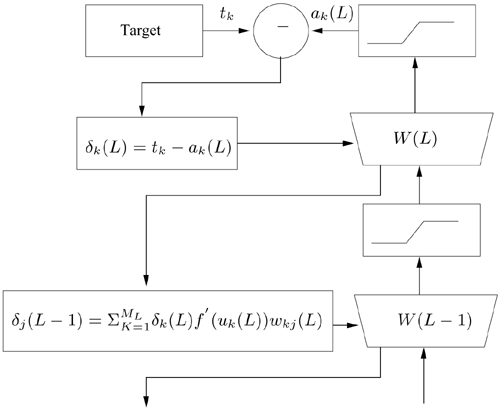
with the initial condition given by Eq. 5.4.3. Figure 5.5 illustrates the BP process.

5.4.2. BP Algorithm for Multi-Layer RBF Networks

In the 1980s, the multi-layer LBF networks trained by the BP algorithm [326] attracted considerable attention from the neural network community. While these networks have shown promise in many application domains, during the last two decades, statisticians and the neural network community found that kernel-based neural networks (or equivalent multi-layer RBF networks) possess a number of advantages over multi-layer LBF networks. These advantages include rapid training speed; better generalization; and more important, the ability to divide a complex task into a number of subtasks (i.e., modularization—see Section 6.3). These positive properties have been demonstrated in multiple theoretical studies and can be found in many real-world applications [186].

In a multi-layer RBF network, each neuron in the hidden-layer is composed of a radial basis function, which also serves as an activation function. The weighting parameters in an RBF network are the centers and widths of these neurons. The output functions are the linear combination of these radial basis functions. A more general form of the RBF networks is the elliptical basis function (EBF) networks where the hidden neurons compute the Mahalanobis distance between the centers and the input vectors. It has been shown that RBF networks have the same asymptotic approximation power as multi-layer LBF networks [279].

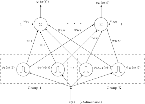
Figure 5.6 depicts the architecture of an RBF/EBF network with D inputs, M-basis functions (hidden nodes), and K outputs (see p. 152). The input layer distributes the D-dimensional input patterns, x⁽ⁿ⁾, to the hidden-layer. Each hidden unit is a Gaussian-basis function of the form

Equation 5.4.10

where µ_j and ∑_j are the mean vector and covariance matrix of the j-th basis function, respectively. The k-th output is a linear weighted sum of the basis functions' outputs; that is,

Equation 5.4.11

where x⁽ⁿ⁾ is the n-th input vector, w_k0 is a bias term, and φ ₀(·) ≡ 1. To apply RBF/EBF networks for pattern classification, each class is assigned a group of hidden units as depicted in Figure 5.6, and each group is trained to represent the patterns belonging to its corresponding class.

In addition to multi-layer LBF networks, the BP algorithm described before can also be applied to multi-layer RBF networks. Denote the mean vector and covariance matrix of the j-th kernel of a multi-layer RBF network as δ_j = [δ_j1, …, δ_jD]^T and Σ_j = diag, respectively, where D is the number of inputs (feature dimension). For a multi-layer RBF network with K outputs, further denote

Equation 5.4.12

as the error between the k-th target output and the k-th actual output, where y_k(x⁽ⁿ⁾) is evaluated using Eqs. 5.4.10 and 5.4.11. The total squared error for all training patterns becomes

Equation 5.4.13

The instantaneous update formulae^[1] for the parameters of the network are defined as:

^[1] They are equivalent to the sequential update mode of the BP algorithm.

Equation 5.4.14

Equation 5.4.15

Equation 5.4.16

where n denotes the presentation of the n-th pattern in a particular epoch. Note that n also serves as the iteration index within an epoch. Referring to the symbols defined in the beginning of Section 5.4, observe that , where L = 2 and f(u_k(L)) = u_k(L). Therefore, based on Eq. 5.4.2, the gradient of the output weights is as follows:

Equation 5.4.17

For the hidden nodes' weights and , observe also that , where f(u) = exp(u) (see Eq. 5.2.4) and has the form

Therefore, one can apply Eqs. 5.4.2 and 5.4.5 to obtain , as follows:

Equation 5.4.18

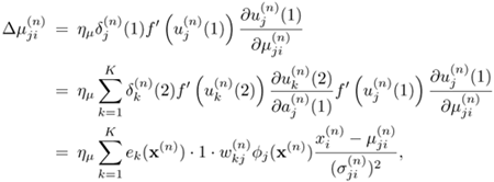
where one has made use of the fact that , , , and . Similarly, is computed as

Equation 5.4.19

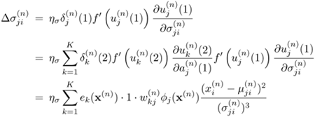
Alternatively, the following gradient descent rules can be directly applied to obtain the same set of update formulae (see Problem 13):

Equation 5.4.20

Equation 5.4.21

Equation 5.4.22

To ensure positivity of σ_ji, define and replace σ_ji in Eq. 5.4.22 with σ_ji; that is,

Note that

results in