
5.7. Biometric Authentication Application Examples
Note that most biometric data can be adequately represented by a mixture of Gaussians, and also that RBF neural networks adopt basically the same type of Gaussian kernels. Therefore, RBF networks are more appealing for biometric applications than LBF networks. In fact, RBF and EBF networks have been used extensively in biometric applications. For instance, Brunelli and Poggio [38] used a special type of RBF network, called the "HyperBF" network, for face recognition and reported a 100% recognition rate on a 47-person database. In a speaker verification task, Mak and Kung [225] demonstrated that EBF networks perform substantially better than their RBF counterparts; and in a speaker identification task, Mak et al. [221, 222] found that RBF networks are superior to LBF networks in terms of both identification accuracy and training time.
In Er et al. [87], RBF neural networks are trained by a hybrid learning algorithm to drastically reduce the dimension of the search space in the gradient paradigm. On the widely used Olivetti Research Laboratory (ORL) face database, the proposed system reportedly achieved excellent performance in terms of both learning efficiency and classification error rates. In Zhang and Guo [401], a modular network structure based on an autoassociative RBF module is applied to face recognition applications based on both the XM2VTS and ORL face database. The scheme achieves highly accurate recognition on both databases. RBF neural networks have also been implemented on embedded systems to provide realtime processing speed for face tracking and identity verification [391].
In Cardinaux et al. [46], MLPs and GMMs were compared in the context of face verification. The comparison is carried out in terms of performance, effectiveness, and practicability. Apart from structural differences, the two approaches use different training criteria; the MLP approach uses a discriminative criterion, while the GMM approach uses a combination of maximum likelihood (ML) and maximum a posteriori (MAP) criteria. Experiments on the XM2VTS database have shown that for low-resolution faces the MLP approach has slightly lower error rates than the GMM approach; however, the GMM approach easily outperforms the MLP approach for high-resolution faces and is significantly more effective for imperfectly located faces. The experiments have also shown that computational requirements of the GMM approach can be significantly smaller than those of the MLP approach, with only a slight decrease in performance.
RBF networks have also been used for speaker verification. For example, in Jiang and Deng [165], a Bayesian approach is applied to speaker verification based on the Gaussian mixture model (GMM). In the Bayesian approach, the verification decision is made by comparing Bayes factors against a critical threshold. An efficient algorithm, using the Viterbi approximation, was proposed to calculate the Bayes's factors for the GMM. According to the reported simulation based on the NIST98 speaker verification evaluation data, the proposed Bayesian approach achieves moderate improvements over a well-trained baseline system using the conventional likelihood ratio test.
A close relative of the RBF clustering scheme is the family of vector quantization (VQ) clustering, since they are both based on the distance metric. In He et al. [129], an evaluation experiment was conducted to compare the codebooks trained by the Linde-Buzo-Grey (LBG), the learning vector quantization (LVQ), and the group vector quantization (GVQ) algorithms. (In GVQ training, speaker codebooks are trained and optimized for vector groups rather than for individual vectors.)
Many examples of applying GAs to face detection and recognition have been reported (e.g., references [15, 155, 156, 180, 275]). A face recognition method using support vector machines with the feature set extracted by genetic algorithms was proposed in Lee et al. [199]. By selecting the feature set with superior performance in face recognition, the use of unnecessary facial information can be avoided and memory requirements can be significantly reduced.
Problems
Consider the classical XOR problem defined in Eq. 5.3.4. Show that
the XOR data can be separated by the following elliptic decision boundary:

they are separable by an even simpler hyperbolic decision boundary:

Verify your answers by using the Matlab function ezplot.m.
This problem again concerns the XOR problem:
Explain why multi-layer networks with nonlinear RBF kernels can be used for separating XOR data.
Repeat the same problem for multi-layer networks with nonlinear LBF kernels.
Compare multi-layer perceptrons and radial basis function networks in the context of
the number of possible hidden-layers
the representation of the hidden nodes' activation
the training time required
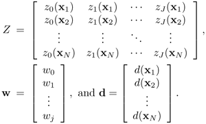
Given N input patterns, the output of a radial basis function network with D inputs, M hidden nodes, one bias term, and one output can be expressed as

where y = [y1, y2, …, yN]T, w = [ω0,ω 1, …, ωM]T, and Φ is an (N x M + 1) matrix with each row containing the hidden nodes' outputs. Assume that N = 3 and M = 2. Assume also that the desired output vector is
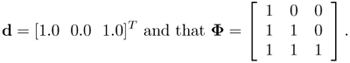
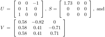
Find the least-squares solution of w if the singular value decomposition of Φ is given by Φ = USVT, where

and S = diag{2.25, 0.80, 0.56}. Hence, find the least-squares error

When only a few training patterns are available, using SVD to determine the output weight matrix W of an RBF network is recommended (see Section 5.5). Explain why, if the amount of training data is large, it may not be necessary to use SVD. Instead, the normal equation

of the linear least-squares problem

will be sufficient to find the output weights. In other words, show that the larger the training set, the more numerically stable the normal equation is. Equivalently, show that
 , where
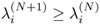
  ) is the i-th singular value for a data collection with N (resp. N + 1) samples. Hint: If
where all matrices are real matrices, show that
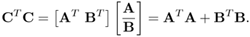
Since BTB is positive semidefinite, therefore, the eigenvalues of CT C are no smaller than that of AT A [116]. Equivalently, the singular values of C are no smaller than that of A. (For a numerical example, see Problem 6.)
Matlab Exercise. It is well known that the SVD approach to solving least-squares problems requires a great deal more computation than using the normal equation. Therefore, SVD should only be used in a critical situation (i.e., if it can make a difference in numerical behavior). The following Matlab code shows that the more training patterns that are available, the more stable is a normal equation's numerical behavior. Therefore, there is less need for the computationally complex SVD algorithm. Verify this statement by using Matlab and varying the vectors a, b, c, and d. (See Figure 5.13.)
clear all; close all;
a=[5 6]'; b=[-3 4]'; c=[4 4]'; d=[-l -4]';
A1 = [a*a']
svd(A1)
plot(svd(A1),'k'),
axis([l 2 0 120]);
hold;
A2 = a*a' + b*b'
svd(A2)
plot(svd(A2),'k--'),
A3 = a*a' + b*b'+ c*c'
svd(A3)
plot(svd(A3),'k-.'),
A4 = a*a' + b*b'+ c*c' + d*d'
svd(A4)
plot(svd(A4),'k:'),
Figure 5.13. Results of the Matlab code shown in Problem 6. The figure shows the increases in the singular values when positive semidefinite matrices are added to a positive semidefinite matrix. The tick marks at the horizontal axis represent the two singular values (λl and λ2) and the vertical axis their numerical values. Solid: λi of A1; dashed: λi of A1 + A2; solid dashed: λi of A1 + A2 + A3; and dotted: λi of A1 + A2 + A3 + A4.

Matlab Exercise. The following Matlab code compares the numerical performance and stability of SVD and the normal equation for finding a least-squares solution.
clear all; close all; echo off;
disp('Without dependent columns of A, press any key to start'),
pause;
A=[1 2; 3 4; 5 6]; d=[-3 2 3]';
w=inv(A'*A)*A'*d;
y=A*w
E=(d-y)'*(d-y)
disp('Poor precision in w, press any key to start') ;pause;
w1 = w + [0.01 -0.01]'*w(1);
y1=A*w1
E1=(d-y)'*(d-y)
disp('With dependent columns of A, press any key to start'),
pause;
A=[1 2; 2 4; 3.0000000001 6]; d=[-3 2 3]';
w=inv(A'*A)*A'*d;
y=A*w
E=(d-y)'*(d-y)
disp('Poor precision in w, press any key to start'),pause;
w1 = w + [0.01 -0.01]'*w(1);
y1=A*w1
E=(d-y1)'*(d-y1)
disp('Solve the normal eq. by SVD, press any key to start'),
pause;
[U,S,V]=svd(A);
invS = S;
for i=1:2,
  if(abs(S(i,i))< 0.0001)
    invS(i,i) = 0.0;
  else
    invS(i,i) = 1/S(i,i);
  end
end
w=V*invS'*U'*d;
y=A*w
E=(d-y)'*(d-y)
disp('Poor precision in w, press any key to start'),pause;
w1 = w + [0.01 -0.01]'*w(1);
y1=A*w1
E=(d-y1)'*(d-y1)
disp('Ignore the second dimension of input data,...
      press any key to start'),pause;
A=[1 ; 2 ; 3.0000000001]; d=[-3 2 3]';
w=inv(A'*A)*A'*d;
y=A*w
E=(d-y)'*(d-y)
Explain why the error E is large when there are dependent columns in matrix A and the precision of w is poor.
Discuss the geometrical interpretation of having a singular value of 0 in matrix S. Hence, explain how the singular value decomposition approach helps avoid the numerical difficulty arising from the singularity of ATA.
An elliptical basis function (EBF) network with M centers, K outputs, and no bias term has the form

where ωkj (k = 1, …, K and j = 1, …, M) are the output weights and φj(x) is the j-th basis function output. An M-center GMM has the form

where
 are the GMM's parameters and pj(·) is the j-th hidden node output. Compare the EBF network and the GMM in the context of their
hidden unit representation
output representation
training algorithm
A fully connected feed-forward multi-layer perceptron network has eight inputs, four outputs, and two hidden layers, one with six hidden nodes and the other with three nodes.
Draw a flow graph of this network.
For the retrieving phase, what is the computational complexity in terms of MACs (multiplier-accumulations)?
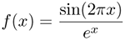
A radial basis function (RBF) network with 10 function centers is applied to approximate the function
shown in Figure 5.14. Suggest appropriate positions for the function centers and explain your suggestions. Verify your answer by using Matlab.
Figure 5.14. Function to be approximated by an RBF network.
What are the advantage(s) and disadvantage(s) of using elliptical basis function networks instead of radial basis function networks for pattern classification?
The k-th output of an RBF network with K outputs has the form
For the case of Gaussian basis functions, there is either
or
where
 and ∑j are the mean vectors and the covariance matrices, respectively, and σj is the function width associated with the j-th cluster.
The outputs of an EBF network with I inputs, J hidden nodes, and K outputs are given by
where

Let the total squared error be
where
 is the desired output for the input vector
  . Derive expressions for
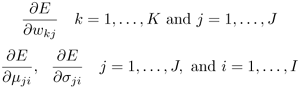
Hence suggest a gradient-based learning rule for the EBF network.
Identify two disadvantages of the gradient-based learning rule derived in Problems 13b and 13c.
Assume that an RBF network with I inputs, J hidden nodes, and one output has a Gaussian-basis function of the form

where cj and σj are the j-th function center and function width, respectively.
Express the output y(xp) in terms of ωj, xpi, cji, and σj, where 1 ≤ i ≤ I, 0 ≤ j ≤ J, 1 ≤ p ≤ N, and N is the number of training pairs {xp, d(xp)}. Note that xpi is the i-th input of the p-th pattern and cji is the position of the j-th center with respect to the i-th coordinate of the input domain.
Show that the total squared error is

where
Hence, show that

State the condition under which (ZTZ)TZTd is susceptible to numerical error.
An RBF network has n inputs, three hidden nodes, and one output. The output of the network is given by

where
 are the activation of the hidden nodes and
  are the weights connecting the hidden nodes and the output node. Table 5.8 shows the relationship among φi(xp), y(xp) and the desired output d(xp) for input vectors
  .
.Determine the matrix A such that Aw = y, where

Express the vector w* that minimizes the error

in terms of A, w, and d. Explain whether you can determine a numerical value of w* by using your expression.
If the singular decomposition of A is equal to USVT, where
suggest a least-squares solution for w*.
Table 5.8. Input Vector φ1(x) φ2(X) φ3(x) d(xp) Actual Output x1 0 0 0 1 y(xi) x2 0 0 0 1 y(x2) X3 1 1 1 0 y(x3) The probability density function of the k-th class is defined as p(x|Ck), where x denotes the vector in the feature space and Ck represents the k-th class.
Use Bayes's theorem to express the posterior probability p(Ck|x) in terms of p(x|Ck) and p(x), where p(x) = ∑ip(x|Ci)P(Ci) is the probability density function of x.
Given that it is possible to use a common pool of M-basis functions
 , labeled by an index j, to represent all of the class-conditional density; that is,
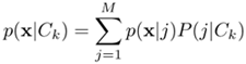
show that
 .
.Hence, show that the basis function outputs and the output weights of an RBF network can be considered as posterior probabilities.
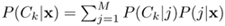
The posterior probability of class Ck in a K-class problem is given by

where
 is a GMM, P(Ck) is the prior probability of class Ck, and p(x) is the density function of x.
Express p(x) in terms of p(x|Ck) and P(Ck).
Discuss the difference between P(Ck) and πkj.
If P(Ck) ≠ P(Cj) ∀k ≠ j, explain how you would use K GMMs to classify a set of unknown pattern X = {x1, x2, …, XT} into K classes.
The BP algorithm involves the computation of the gradient
 , where E is the mean-squared error between the desired outputs and the actual outputs and wij(l) is the weights at layer l.
Repeat (a) for a multi-layer RBF network using Eq. 5.2.2 and the back-propagation rule for multi-layer RBF networks (Eq. 5.4.17-Eq. 5.4.19).
Derive the gradient of a Gaussian EBF in Eq. 5.4.10.
Assume that you are given a set of data with an XOR-type distribution: For one class there are two centroids located at (0,0) and (1,1), while for the other class there are two centroids located at (1,0) and (0,1). Each cluster can be statistically modeled by a uniform distribution within a disk of radius r = 1.
Show that the two classes are not linearly separable.
Derive an analytical solution (equations for the decision boundaries) for a multi-layer LBF network (no computer).
Verify your solutions using Matlab and Netlab.
The implementation cost of multi-layer neural models depends very much on the computational complexity incurred in each layer of feed-forward processing. Compute the number of multiplications and additions involved when a 3 x 4 matrix is postmultiplied by a 4 x 12 matrix.
Is it true that the basis function of kernel-based networks must be in the form of a Gaussian function? Provide an explanation. Note: RBF networks are considered to be one type of kernel-based networks.
Multiple Choice Questions:
The outputs of an RBF network are linear with respect to
the inputs
the weights connecting the hidden nodes and the outputs
parameters of the hidden nodes
the outputs of the hidden nodes
both (ii) and (iv)
none of the above
The purpose of the function width σ in an RBF network is to
improve the numerical stability of the K-means algorithm
allow the basis functions to cover a wider area of the input space so that better generalization can be achieved
ensure that the inference of the individual-basis functions will not overlap with each other
none of the above
To train an RBF network, one should apply the K-means, least-squares, and K-nearest-neighbor algorithms in the following order:
K-means, least squares, K-nearest neighbor
K-means, K-nearest-neighbor, least squares
Least squares, K-means, K-nearest neighbor
Least squares, K-means, and K-nearest-neighbor in any order
To apply singular value decomposition to determine the output weights of an RBF network,
decompose matrix A into A = UAVT, where A = {api} = {Φi (||xp – ci||)} contains the basis function outputs and Λ = diag {λ1, λ2, ..., λd} contains the singular values
set 1/λj = 0 if λj → 0
set λj = 0 if λj → ∞
both (i) and (ii)
both (i) and (iii)
Given the decision boundaries and the contours of basis function outputs of Figure 5.15, it is correct to say that
The figure is produced by an RBF network with 2 centers.
The figure is produced by an RBF network with 4 centers.
The figure is produced by an EBF network with 4 centers.
The figure is produced by an EBF network with 2 centers.
Based on the figure in the preceding question, it is correct to say that
The covariance matrix corresponding to Class 1 (4th quadrant) is diagonal.
The covariance matrix corresponding to Class 2 (3rd quadrant) is not diagonal.
The covariance matrix corresponding to Class 1 (2nd quadrant) exhibits a larger variance along the horizontal axis.
All of the above.
In the context of pattern classification, RBF outputs can be trained to give
the posterior probabilities of class membership, P(Ck|x)
the likelihood of observing the input data given the class membership, p(x|Ck)
the likelihood of observing the input data, p(x)
both (i) and (ii)
(i), (ii), and (iii)
Training of RBF networks is usually faster than training multi-layer perceptrons because
Training in RBF networks is divided into two stages, where each stage focuses on a part of the optimization problem.
RBF networks have fewer parameters to be estimated.
The RBF networks' outputs are linear with respect to all of the networks' parameters.
None of the above.
Training of RBF networks requires a large amount of memory because
Answers: a (v), b (ii), c (ii), d (iv), e (iii), f (iv), g (i), h (i), i (ii)
Matlab Exercise. Given two classes of patterns with distributions p1(x, y) and P2(x, y), where for p1 the mean and variance are, respectively,

and for p2 the mean and variance are

write Matlab code to generate 1,000 patterns for each distribution. Create an RBF network and a GMM-based classifier to classify the data in these two classes. For each network type, find the classification accuracy and plot the decision boundary.
Matlab Exercise. Create 100 two-dimensional data patterns for two classes. Use an RBF BP Network to separate the two classes. Try to do clustering by using
an RBF BP network with four hidden units
an EBF BP network with four hidden units
