5.5. Two-Stage Training Algorithms

The convergence behavior of the BP algorithm for multi-layer networks has always been an issue of great concern. This is because the algorithm tends to be sensitive to initial conditions. Therefore, the convergence problem can be greatly alleviated if proper initial conditions can be estimated. This motivates the two-stage training strategy discussed next.

5.5.1. Two-Stage Training for RBF Networks

The two-stage training of RBF networks starts with the estimation of the kernel means using the K-means algorithm

Equation 5.5.1

Equation 5.5.2

where

Equation 5.5.3

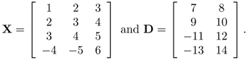
N_j is the number of patterns in the cluster X_j, and || · || is the Euclidean norm. After the kernel parameters are determined, the kernel outputs {φ_j (x⁽ⁿ⁾); j = 0,_'…, M} are computed using the input/teacher training pairs {x⁽ⁿ⁾, d⁽ⁿ⁾} to form the matrix equation

Equation 5.5.4

where

Therefore, the training of the output weights amounts to finding the inverse of Φ. However, in most cases, Φ is not a square matrix. For a small amount of training data, a reliable way to solve Eq. 5.5.4 is to use the technique of singular value decomposition [285]. In this approach, the matrix Φ is decomposed into the product UΛV^T, where U is an N x (M + 1) column-orthogonal matrix, Λ is an (M + 1) x (M + 1) diagonal matrix containing the singular values, and V is an (M + 1) x (M + 1) orthogonal matrix. The weight vectors are given by

Equation 5.5.5

where d_k is the k-th column of D and Λ = diag{λ₀, …, λ_M} contains the singular values of Φ. To ensure numerical stability, set 1/λ_i to zero for those λ_i less than a machine-dependent precision threshold. This approach effectively removes the effect of the corresponding dependent columns in Φ. For an over determined system, singular value decomposition gives a solution that is the best approximation in the least squares sense. On the other hand, when the amount of training data are sufficiently large to ensure that Φ is of full rank, the squared error between the actual output and the desired output can be minimized:

to give the normal equations of the form

Equation 5.5.6

Compared to the gradient-based training scheme for multi-layer RBF networks described before, the two-stage training approach has two advantages:

Probabilistic Interpretation

Research has found that RBF networks are capable of estimating Bayesian posterior probabilities [311]. In fact, the link of RBF networks with statistical inference methods is more obvious than that of the LBF networks.

As noted in Section 5.2, each hidden neuron in an RBF network feeds the inputs into the radial basis function (Eq. 5.2.2) and generates the output using the Gaussian activation function (Eq. 5.2.4). For example, the output of the j-th neuron is given by

Equation 5.5.7

where x is a D-dimensional input vector. Usually the vector w_j is a randomly selected input pattern, but it would be more efficient to use the mean vector to represent multiple patterns of the same cluster. Also, the spread parameter σ can be extended to a covariance matrix ∑ so that the neuron has more flexibility.

The network output k is a linear combination of the hidden neurons' outputs:

Equation 5.5.8

where w = {w₁, w₂, …, w_M} are the parameters (means and covariances) of the M-hidden neurons, and π_kj specifies the connection weight between output neuron k and hidden neuron j. Note that RBF networks are closely related to the Parzen windows approach [270] in that the estimated class-conditional densities are a linear superposition of window functions—one for each training pattern. Moreover, if the weighting parameters π_js follow the constraints ∑_j π_kj = 1 and π_kj ≥ 0 ∀_j and k, RBF networks are similar to the mixture of Gaussian distributions. Richard and Lippmann [311] have shown that if the output values of an RBF network are limited to [0,1], then with a large enough training set, the network outputs approximate the Bayesian posterior probabilities. Since most RBF learning schemes do not restrict the output values to [0,1], Bridle [35] suggested normalizing the outputs by a softmax-type function of the form:

Equation 5.5.9

According to Eq. 5.5.8, if f_i (w_j, x) is a density function,φk(w, x) will also be a density function. As a result, one can write the posterior probability of class ω_k as

Equation 5.5.10

Comparing Eq. 5.5.9 with Eq. 5.5.10, one can see that the normalized RBF network outputs approximate the posterior probabilities with the assumption that p(ω_i) = P(ω_i) = P(ω_j), ∀i, j.

RBF Networks versus EBF Networks

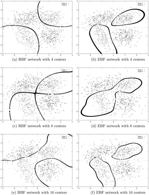
Notice that when in Eq. 5.4.10, the EBF network reduces to an RBF network. Although RBF networks have fewer parameters than EBF networks; their disadvantage is that they usually require a larger number of function centers to achieve similar performance [220]. The major reason is that, in EBF networks, each basis function has a full covariance matrix or a diagonal covariance matrix with different variances for each component, which forms a better representation of the probability density function; whereas in RBF networks, the distribution is modeled by a collection of diagonal covariance matrices with equal variances. Figure 5.7 shows the decision boundaries and contour lines of the basis functions formed by RBF and EBF networks with various numbers of function centers. The objective is to classify four Gaussian clusters with mean vectors and covariance matrices, as shown in Table 5.1, into two classes. This can be considered as a noisy XOR problem in which the noise components in the input domain are interdependent.

Table 5.1. Mean vectors and covariance matrices of the four clusters in the noisy XOR problem. Each cluster contains 500 samples.

Class 1		Class 2
Mean vector	Covariance matrix	Mean vector	Covariance matrix

Figures 5.7(a) and 5.7(b) indicate that the boundaries formed by the EBF network with four centers are better for modeling the noise source characteristic than that formed by the RBF networks. Table 5.2 shows the recognition accuracy obtained by the RBF networks and the EBF networks. The accuracy is based on 2,000 test vectors drawn from the same population as the training set. The result demonstrates that the EBF networks can attain higher recognition accuracy than the RBF networks. It also suggests that increasing the size of the RBF networks could slightly increase recognition accuracy, but recognition accuracy is still lower than that of the EBF network with the smallest size (compare 90.57% with 91.14%). Increasing the number of function centers will also make the decision boundaries unnecessarily complicated, as shown in Figures 5.7(e) and 5.7(f).

Table 5.2. Recognition accuracy achieved by the RBF and the EBF networks in the noisy XOR problem. All figures are based on five simulation runs with different initial conditions. N_rbf and N_ebf denote the numbers of free parameters in the RBF and EBF networks, respectively.

Number of Centers	RBF Network		EBF Network
	Nrbf	Rec. accuracy	Nebf	Rec. accuracy
4	22	88.47%	30	91.14%
8	42	90.57%	58	90.87%
16	82	89.77%	114	90.86%

5.5.2. Two-Stage Training for LBF Networks

The two-stage training approach just discussed can also be applied to train multilayer LBF networks. Here a two-layer LBF network is used to illustrate the procedure. Recall from Section 5.4 that the outputs of a three-layer LBF network (i.e., L = 2) is

Equation 5.5.11

where f (·) is a nonlinear activation function.^[2] In matrix form, Eq. 5.5.11 can be written as Y = XH, where Y is an N × K matrix, X is an N × D matrix, and H is an D × K matrix. The weight matrix W is the least-squares solution of the matrix equation

^[2] For simplicity, the bias terms in Eq. 5.5.11 have been ignored.

Equation 5.5.12

where D is an N × K target matrix containing the desired output vectors in its rows.

As X is not a square matrix, its left-inverse is

Equation 5.5.13

So ideally, this is

Equation 5.5.14

Assuming that the number of hidden units M is less than that of the input, then H can be approximated by a rank M-matrix factorization:

Equation 5.5.15

where W(1) and W(2) are, respectively, D x M and M x K weight matrices corresponding to Layer 1 and Layer 2.

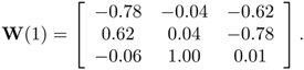
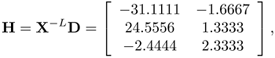
Suppose that the singular value decomposition of H = X^-LD can be decomposed (approximately) into the product X^-LD ≈ UΛV^T, where U is a D x M column-orthogonal matrix, Λ is an M x M diagonal matrix containing the singular values, and V is an M x K orthogonal matrix. The weight matrix W(1) is given by W(1) = U, and the output of the hidden units will be f(XW(1)), where f(·) stands for the nonlinear activation function. Having derived the initial values for the hidden units, the derivation for the upper-layer W(2) follows the same approach as that adopted in the RBF case. In other words, the kernel outputs are again computed to form the matrix equation (5.5.4). Then, the output weights are computed using SVD.

As a numerical example, let

Then,

which can be decomposed into

Hence, W(1) can be initialized to