Reliability

Reliability is a key advantage of distributed systems. Imagine if you have a single computer. Then, when it fails, there is no choice but to reboot it or get a new one if it had developed a significant fault. However, there are multiple nodes in distributed systems in a system that allows a distributed system to tolerate faults up to a level. Thus, even if some computers fail in a distributed network, the distributed system keeps functioning. Reliability is one of the significant areas of study and research in distributed computing, and we will look at it in more detail in the context of fault tolerance shortly.

Performance

In distributed systems, better performance can be achieved naturally. For example, in the case of a cluster of computers working together, better performance can be achieved by parallelizing the computation. Also, in a geographically dispersed distributed network, clients (users) accessing nodes can get data from the node which is closer to their geographic region, which results in quicker data access. For example, in the case of Internet file download, a mirror that is closer to your geographic region will provide much better download speed as compared to the one that might be in another continent.

Performance of a distributed system generally encompasses two facets, responsiveness and throughput.

Resource Sharing

Resources in a distributed system can be shared with other nodes/participants in the distributed system. Sometimes, there are expensive resources such as a supercomputer, a quantum computer, or some industrial grade printer which can be too expensive to be made available at each site; in that case, resources can be shared via communication links to other nodes remotely. Another scenario could be where data can be divided into multiple partitions (shards) to enable quick access.

Inherently Distributed

There are scenarios where there is no option but to build a distributed system because the problem can only be solved by a distributed system. For example, a messaging system is inherently distributed. Mobile network is inherently by nature distributed. In these and similar use cases, a distributed system is the only one that can solve the problem; therefore, the system has to be distributed by design.

With all these benefits of distributed systems, there are some challenges that need to be addressed when building distributed systems. The properties of distributed systems such as no access to a global clock, asynchrony, and partial failures make designing reliable distributed systems a difficult task. In the next section, we look at some of the primary challenges that should be addressed while building distributed systems.

Fault Tolerance

With more computers and at times 100s of thousands in a data center, for example, in the case of cloud computing, inevitably something somewhere would be failing. In other words, the probability of failing some part of the distributed system, be it a network cable, a processor, or some other hardware, increases with the number of computers. This aspect of distributed systems requires that even if some parts of the distributed system fail (usually a certain threshold), the distributed system as a whole must keep operating. To this end, there are various problems that are studied in distributed computing under the umbrella of fault tolerance. Fault-tolerant consensus is one such example where the efforts are made to build consensus algorithms that continue to run correctly as specified even in the presence of a threshold of faulty nodes or links in a distributed system. We will see more details about that in Chapter 3.

A relevant area of study is failure detection which is concerned with the development of algorithms that attempt to detect faults in a distributed system. This is especially an area of concern in asynchronous distributed systems where there is no upper bound on the message delivery times. The problem becomes even more tricky when there is no way to distinguish between a failed node and a node that is simply slower and a lost message on the link. Failure detection algorithms give a probabilistic indication about the failure of a process. This up or down status of the node then can be used to handle that fault.

Another area of study is replication which provides fault tolerance on the principle that if the same data is replicated across multiple nodes in a distributed system, then even if some nodes go down the data is still available, which helps to keep the system stable and continue to meet its specification (guarantees) and remain available to the end users. We will see more about replication in Chapter 3.

Security

Being a distributed system with multiple users using it, out of which some might be malicious, the security of distributed systems becomes a prime concern. This situation is even more critical in geographically dispersed distributed systems and open systems such as blockchains, for example, Bitcoin blockchain. To this, the fundamental science used for providing security in distributed systems is cryptography, which we will cover in detail in Chapter 2, and we will keep referring to it throughout the book, especially in relation to blockchain consensus. Here, we study topics such as cryptography and address challenges such as authentication, confidentiality, access control, nonrepudiation, and data integrity.

Heterogeneity

A distributed system is not necessarily composed of exactly the same hardware nodes. It is possible and is called homogenous distributed system, but usually the hardware and operating systems are different from each other. In this type of scenario, different operating systems and hardware can behave differently, leading to synchronization complexities. Some nodes might be slow, running a different operating system which could have bugs, some might run faster due to better hardware, and some could be resource constrained as mobile devices or IoT devices. With all these different types of nodes (processes, computers) in a distributed system, it becomes challenging to build a distributed algorithm that works correctly on all these different types of systems and continues to operate correctly despite the differences in the local operating environment of the nodes.

Distribution Transparency

One of the goals of a distributed system is to achieve transparency. It means that the distributed system, no matter how many individual computers and peripherals it is built of, it should appear as a single coherent system to the end user. For example, an ecommerce website may have many database servers, firewalls, web servers, load balancers, and many other elements in their distributed system, but all that should be abstracted away from the end user. The end user is not necessarily concerned about these backend "irrelevant" details but only that when they make a request, the system responds. In summary, the distributed system is coherent if it behaves in accordance with the expectation of the end user, despite its heterogeneous and dispersed structure. For example, think about IPFS, a distributed file system. Even though the files are spread and sharded across multiple computers in the IPFS network, to the end user all that detail is transparent, and the end user operates on it almost as if they are using a local file system. Similar observation can be made about other systems such as online email platforms and cloud storage services.

Timing and Synchronization

Synchronization is a vital operation of a distributed system to ensure a stable global state. As each process has its view of time depending on their internal physical clocks which can drift apart, the time synchronization becomes one of the fundamental issues to address in designing distributed systems. We will see some more details around this interesting problem and will explore some solutions in our section on timing, orders, and clocks in this chapter.

Global State

As the processes in a distributed system only have knowledge of their local states, it becomes quite a challenge to ascertain the global state of the system. There are several algorithms that can be used to do that, such as the Chandy-Lamport algorithm. We will briefly touch upon that shortly.

Concurrency

Concurrency means multiple processes running at the same time. There is also a distinction made between logical and physical concurrency. Logical concurrency refers to the situation when multiple programs are executed in an interleaving manner on a single processor. Physical concurrency is where program units from the same program execute at the same time on two or more processors.

Distributed systems are ubiquitous. They are in everyday use and have become part of our daily routine as a society. Be it the Internet, the World Wide Web, Bitcoin, Ethereum, Google, Facebook, or Twitter, distributed systems are now part of our daily lives. At the core of distributed systems, there are distributed algorithms which form the foundation of the processing being performed by the distributed system. Each process runs the same copy of the algorithm that intends to solve the problem for which the distributed system has been developed, hence the term distributed algorithm.

A process can be a computer, an IoT device, or a node in a data center. We abstract these devices and represent these as processes, whereas physically it can be any physical computer.

Now let’s see some of the relevant technologies and terminologies.

Processes

A process in a distributed system is a computer that executes the distributed algorithm. It is also called a node. It is an autonomous computer that can fail independently and can communicate with other nodes in the distributed network by sending and receiving messages.

Events

The diagram shown in Figure 1-5 presents this visually.

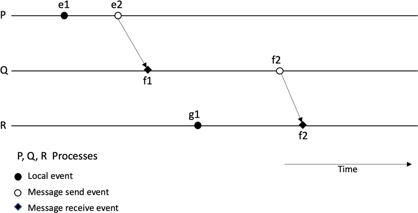
A schematic with 3 lines, P, Q, and R, has events like local, message sent, and message received. Some of the events are connected together via time.

State

The concept of state is critical in distributed systems. You will come across this term quite a lot in this book and other texts on distributed systems, especially in the context of distributed consensus. Events make up the local state of a node. In other words, a state is composed of events (results of events) in a node. Or we can say that the contents of the local memory, storage, and program as a result of events make up the process’s state.

Global State

The collection of states in all processes and communication links in a distributed system is called a global state.

This is also known as configuration which can be defined as follows:

The configuration of a distributed system is composed of states of the processes and messages in transit.

Execution

Cuts

A cut can be defined as a line joining a single point in time on each process line in a space-time diagram. Cuts on a space-time diagram can serve as a way of visualizing the global state (at that cut) of a distributed computation. Also, it serves as a way to visualize what set of events occurred before and after the cut, that is, in the past or future. All events on the left of the cut are considered past, and all events on the right side of the cut are said to be future. There are consistent cuts and inconsistent cuts. If all received messages are sent within the elapsed time before the cut, that is, the past, it is called a consistent cut. In other words, a cut that obeys causality rules is a consistent cut. An inconsistent cut is where a message crosses the cut from the future (right side of the cut) to the past (left side of the cut).

If a cut crosses over a message from the past to the future, it is a graphical representation of messages in transit.

The diagram shown in Figure 1-6 illustrates this concept, where C₁ is an inconsistent cut and C₂ is a consistent cut.

A schematic with 3 lines, P, Q, and R, has events like E P 1, E P 2, and so on. All the events are grouped into 2 cuts labeled C 1 and C 2.

Algorithms such as the Chandy-Lamport snapshot algorithm are used to create a consistent cut of a distributed system.

Taking a snapshot of a distributed system is helpful in creating a global picture of the system. A snapshot or global snapshot captures the global state of the system containing the local state of each process and the individual state of each communication link in the system. Such snapshots are very useful for debugging, checkpointing, and monitoring purposes. A simple solution is to synchronize all clocks and create a snapshot at a specific time, but accurate clock synchronization is not possible, and we can use causality to achieve such an algorithm that gives us a global snapshot.

Note that any process can initiate the snapshot, the algorithm does not interfere with the normal operation of the distributed system, and each process records the state of incoming channels and its own.

Client-Server

This model is a common way to have two processes work together. A process assumes the role of a client, and the other process assumes the role of a server. The server receives requests made by the client and responds with a reply. There can be multiple client processes but only a single server process. For example, a classic web client and web server (browser to a web server) design follows this type of architecture. Figure 1-7 depicts the so-called physical view of this type of architecture.

A schematic of a server connected to 3 clients. The request is sent from the client to the server, and a reply is sent from the server to the client.

Multiserver

A multiserver architecture is where multiple servers work together. In one style of architecture, the server in the client-server model can itself become a client of another server. For example, if I have made a request from my web browser to a web server to find prices of different stocks, it is possible that the web server now makes a request to the backend database server or, via a web service, requests this pricing information from some other server. In this scenario, the web server itself has become a client. This type of architecture can be seen as a multiserver architecture.

Another quite common scenario is where multiple servers act together to provide a service to a client, for example, multiple database servers providing data to a web server. There are two usual methods to implement such collaborative architecture. The first is data partitioning, and another is data replication. Another closely related term to data partitioning is data sharding.

Data partition refers to an architecture where data is distributed among the nodes in a distributed system, and each node becomes responsible for its partition (section) of the data. Partitioning of data helps to achieve better performance, easier administration, load balancing, and better availability. For example, data for each department of a company can be divided into partitions and stored separately on different local servers. Another way of looking at it is that if we have a large table with one million rows, I might put half a million rows on one server and another half on another server. This scheme is called data sharding or horizontal partitioning, or horizontal sharding depending on how the sharding is performed.

We can visualize the concept of partitioning in Figure 1-8.

A schematic of data partitioning. Citizen database from all regions are connected to regional offices at London, Bradford, and Montgomery

Note that data partitioning shown in Figure 1-8 is where a large central database is partitioned into smaller datasets relevant to each region, and a regional server then manages the partition. However, in another type of partitioning, a large table can be partitioned into different tables, but it remains on the same physical server. It is called logical partitioning.

A shard is a horizontal partition of data where each shard (fragment) resides on a separate server. One immediate benefit of such an approach is load balancing to spread the load between servers. This concept is shown in Figure 1-9.

A set of 5 tables. A table at the top is titled table. 2 tables are titled vertical shards and 2 are titled horizontal shards.

Data replication refers to an architecture where each node in the distributed system holds an identical copy of the data. A typical simple example is that of the RAID 0 system; while they are not separate physical servers, the data is replicated across two disks, which makes it a data replication (commonly called mirroring) architecture. In another scenario, a database server might run a replication service to replicate data across multiple servers. This type of architecture allows for better performance, fault tolerance, and higher availability. A specific type of replication and fundamental concept in a distributed system is state machine replication used to build fault-tolerant distributed systems. We will cover more about this in Chapter 3.

Figure 1-10 shows multiserver architectures where a variation of the client-server model is shown. The server can act as a client to another server. This is another approach where multiple servers work together closely to provide a service.

A schematic with connected servers and a client. Another client at the bottom sends a request and receives a reply.

Another diagram in Figure 1-11 shows the concept of data replication.

A schematic of data replication. The citizen database at the headquarters is connected to 3 citizen databases at the regional offices.

In summary, replication refers to a practice where a copy of the same data is kept on multiple different nodes, whereas partitioning refers to a practice where data is split into smaller subsets, and these smaller subsets are then distributed across different nodes.

Proxy Servers

A proxy server–based architecture allows for intermediation between clients and backend servers. A proxy server can receive the request from the clients and forward it to the backend servers (most commonly, web servers). In addition, proxy servers can interpret client requests and forward them to the servers after processing them. This processing can include applying some rules to the request, perhaps anonymizing the request by removing the client’s IP address. From a client’s perspective, using proxy servers can improve performance by caching. These servers are usually used in enterprise settings where corporate policies and security measures are applied to all web traffic going in or out of the organization. For example, if some websites need to be blocked, administrators can use a proxy server to do just that where all requests go through the proxy server, and any requests for blocked sites are intercepted, logged, and ignored.

The diagram in Figure 1-12 shows a proxy architecture.

A schematic. The client receives a request from a proxy server and sends its reply. The proxy server is connected to 2 other servers.

Peer to Peer

In the peer-to-peer architecture, the nodes do not have specific client or server roles. They have equal roles. There is no single client or a server. Instead, each node can play either a client or a server role, depending on the situation. The fact that all nodes have an equal role resulted in the term "peer."

Peer-to-peer architecture is shown in the diagram in Figure 1-13.

A schematic of peer architecture. 4 peers are connected together via arrows labeled request and reply.

In some scenarios, it is also possible that not all nodes have equal roles; some may act as servers and clients to each other. Generally, however, all nodes have the same role in a peer-to-peer network.

Now that we have covered some architectural styles of distributed systems, let’s focus on a more theoretical side of the distributed system, which focuses on the abstract view of the distributed systems. First, we explore the distributed system model.

Processes

A process or node is a fundamental element in a distributed system which runs the distributed algorithm to achieve that common goal for which the distributed system has been designed.

Now imagine what a process can do in a distributed system. First, let’s think about a normal scenario. If a process is behaving according to the algorithm without any failures, then it is called a correct process or honest process. So, in our model we say that a node running correctly is one of the behaviors a node can exhibit. What else? Yes, of course, it can fail. If a node fails, we say it’s faulty; if not, then it is nonfaulty or correct or honest.

Network

In a distributed network, links (communication links) are responsible for passing messages, that is, take messages from nodes and send to others. Usually, the assumption is a bidirectional point-to-point connection between nodes.

A network partition is a scenario where the network link becomes unavailable for some finite time between two groups of nodes. In practice, this could be due to a data center not speaking to another or an incorrect/unintentional or even intentional/malicious firewall rule prohibiting connections from one part of the network to another.

Synchronous

A synchronous distributed system has a known upper bound on the time it takes for a message to reach a node. This situation is ideal. However, in practice, messages can sometimes be delayed. Even in a perfect network, there are several factors, such as network link quality, network latency, message loss, processing speed, or capacity of the processors, which can adversely affect the delivery of the message.

In practice, synchronous systems exist, for example, a system on a chip (SoC), embedded systems, etc.

Asynchronous

Asynchronous distributed systems are on the other end of the spectrum. In this model, there is no timing assumption made regarding the timing. In other words, there is no upper bound on the time it takes to deliver a message. There can be arbitrarily long and unbounded delays in message delivery or processing in a node. The processes can run at different speeds.

Also, a process can arbitrarily pause or delay the execution or can process faster than other processes. You can probably imagine now that distributed algorithms designed for such a system can be very robust and resilient. However, many problems cannot be solved in an asynchronous distributed system. A whole class of results called "impossibility results" captures the unsolvable problems in distributed systems. We will look at impossibility results in more detail later in the chapter and then in Chapter 3. As several types of problems cannot be solved in an asynchronous model and the synchronous model is too idealistic, we have to compromise. The compromise is called a partially synchronous network.

Partially Synchronous

A partially synchronous model captures the assumption that the network is primarily synchronous and well behaved, but it can sometimes behave asynchronously. For example, processing speeds can differ, or network delays can occur, but the system ultimately returns to a synchronous state to resume normal operation.

Another way to think about this is that the network usually is synchronous but can unpredictably, for a bounded amount of time, behave asynchronously, but there are long enough periods of synchrony where the system behaves correctly.

Another way to think about this is that the real systems are synchronous most of the time but can behave arbitrarily and unpredictably asynchronous at times. During the synchronous period, the system is able to make decisions and terminate.

Figure 1-15 shows how a partially synchronous network behaves.

A graph plots processor delay versus time with a sinusoidal curve. The curve is sectioned as synchronous and asynchronous.

Eventually Synchronous

In the eventually synchronous version of partial synchrony, the system can be initially asynchronous, but there is an unknown time called global stabilization time (GST), unknown to processors, after which the system eventually becomes synchronous. Also, it does not mean that the system will forever remain synchronous after GST. That is not possible practically, but the system is synchronous for a long enough period after GST to make a decision and terminate.

We can visualize the spectrum of synchrony models from asynchronous to synchronous in Figure 1-16.

A schematic with a double-headed arrow labeled synchronous on the right and asynchronous on the left, with partially synchronous in the center.

Both message delivery delay and relative speed of the processes are taken into consideration in synchrony models.

Formal Definitions

Some formal definitions regarding the partial synchrony model are stated as follows:

• Delta Δ denotes a fixed upper bound on the time required for a message to reach from one processor to another.

• Phi Φ denotes a fixed upper bound on the relative speed of different processors.

• GST is the global stabilization time after which the system behaves synchronously.

With these preceding variables defined, we can define various models of synchrony as follows:

• Asynchronous systems are those where no fixed upper bounds Δ and Φ exist.

• Synchronous systems are those where fixed upper bounds Δ and Φ are known.

Partially synchronous systems can be defined in several ways:

• Where fixed upper bounds Δ and Φ exist, but they are not known.

• Where fixed upper bounds Δ and Φ are known but hold after some unknown time T. This is the eventually synchronous model. We can say that eventually synchronous model is where fixed upper bounds Δ and Φ are known but only hold after some time, known as GST.

• In another variation after GST Δ holds for long enough to allow the protocol to terminate.

We will use synchrony models more formally in Chapter 3 in the context of circumventing FLP and consensus protocols. For now, as a foundation the concepts introduced earlier are sufficient.

Figure 1-17 shows synchronous vs. asynchronous communication using a space-time diagram.

Two schematics each with 3 lines, P, Q, and R, and multi-directional arrows. The right has no upper bounds and the left has known upper bounds.

Now that we have discussed the synchrony model, let’s now turn our attention to the adversary model, which allows us to make assumptions about the effect of adversary on a distributed system. In this model, we model how an adversary can behave and what powers an adversary may have in order to adversely influence the distributed system.

Adversary Model

In addition to assumptions about synchrony and timing in a distributed system model, there is another model where assumptions about the power of the adversary and how it can adversely affect the distributed system are made. This is an important model which allows a distributed system designer to reason about different properties of the distributed system while facing the adversary. For example, a distributed algorithm is guaranteed to work correctly only if less than half of the nodes are controlled by a malicious adversary. Therefore, adversary models are usually modelled with a limit to what an adversary can do. But, if an adversary is assumed to be all-powerful who can do anything and control all nodes and communication links, then there is no guarantee that the system will ever work correctly.

Adversary models can be divided into different types depending on the distributed system and the influence they can have on the distributed system and adversely affect them.

In this model, it is assumed there is an external entity that has corrupted the processes and can control and coordinate faulty processes’ actions. This entity is called an adversary. Note that there is a slight difference compared to the failure model here because, in the failure model, the nodes can fail for all sorts of reasons, but no external entity is assumed to take control of processes.

Adversaries can affect a distributed system in several ways. A system designer using an adversary model considers factors such as the type of corruption, time of corruption, and extent of corruption (how many processes simultaneously). In addition, computational power available to the adversary, visibility, and adaptability of the adversary are also considered. The adversary model also allows designers to specify to what limit the number of processes in a network can be corrupted.

We will briefly discuss these types here.

Clock Skew vs. Drift

Due to environmental factors such as temperature and manufacturing differences, quartz crystal clocks can slow down, resulting in skew and drift. The immediate difference between the time shown by two clocks is called their skew, whereas the rate at which two clocks count time differently is called drift. Note that the difference between physical clocks between nodes in a heterogeneous distributed system may be even more significant than homogenous distributed systems where hardware, OS, and architecture are the same for all nodes.

Generally, it is expected that roughly a drift of one second over 11 days can develop, which over time can lead to an observable and significant difference. Imagine two servers running in a data center with no clock synchronization mechanism and are only dependent on their internal quartz clock. In a month, they will be running two to three seconds apart from each other. All time-dependent operations will run three seconds apart, and over time this will continue to worsen. For example, a batch job that is supposed to start at 11 AM will begin at 11 + 3 seconds in a month. This situation can cause issues with time-dependent jobs, can cause security issues, and can impact time-sensitive operations, and software may fail or depict an arbitrary behavior. A much more accurate clock than a quartz clock is an atomic clock.

Atomic Clocks

Atomic clocks are based on the quantum mechanical properties of atoms. Atoms such as cesium or rubidium and mercury are used, and resonant frequencies (oscillations) of atoms are used to record accurate and precise times.

Our notion of time is based on astronomical observations such as changing seasons and the Earth’s rotation. The higher the oscillation, the higher the frequency and the more precise the time. This is the principle on which atomic clocks work and produce highly precise time.

In 1967, the unit of time was defined as a second of “the duration of 9,192,631,770 periods of the radiation corresponding to the transition between the two hyperfine levels of the ground state of the caesium-133 atom.” In other words, oscillation of cesium atoms between two energy states exactly 9,192,631,770 times under controlled environment defines a true second. An atomic clock is shown in Figure 1-22.

A set of 6 of the Cesium Beam atomic clocks with various electrical racks. They have a printout halfway through their height.

Now imagine a scenario where we discover a clock skew and see that one clock is running behind ten seconds. We can usually and simply advance it to ten seconds to make the clock accurate again. It is not ideal but not as bad as the clock skew, where we may discover a clock to run ten seconds behind. What can we do in that case? Can we simply push it back to ten seconds? It is not a very good idea because we can then run into situations where it would appear that a message is received before we sent it.

To address clock skews and drifts, we can synchronize clocks with a trusted and accurate time source.

You might be wondering why there is such a requirement for more and more precise clocks and sources of time. Quartz clocks are good enough for day-to-day use; then we saw GPS as a more accurate time source, and then we saw atomic clocks that are even more accurate and can drift only a second in about 300 million years!¹ But why do we need such highly accurate clocks? The answer is that for day-to-day use, it doesn’t matter. If the time on my wristwatch is a few seconds different from other clocks, it’s not a problem. If my post on a social media site has a timestamp that is a few seconds apart from the exact time I posted it, perhaps that is not an issue. Of course, as long as the sequence is maintained, the timestamp is acceptable within a few seconds. But the situation changes in many other practical scenarios and distributed systems. For example, high-frequency trading systems require (by regulation MiFID II) that the mechanism format the timestamp on messages in the trading system in microseconds and be accurate within 100 microseconds. From a clock synchronization point of view, only 100 microseconds divergence is allowed from UTC. While such requirements are essential for the proper functioning and regulation of the trading systems, they also pose technical challenges. In such scenarios, the choice of source of accurate time, choice of synchronization algorithms, and handling of skews and drifts become of prime importance.

You can see specific MiFID requirements here as a reference:

https://ec.europa.eu/finance/securities/docs/isd/mifid/rts/160607-rts-25-annex_en.pdf

There are other applications of atomic clocks in defense, geology, astronomy, navigation, and many others.

Recently, Sapphire clocks have been developed, which are much more precise than even cesium-based atomic clocks. It is so precise that it can lose or gain a second in three billion years.

Usually, there are two ways in which time is represented in computers. One is epoch time, also called Unix time, which is defined as the number of seconds elapsed since January 1, 1970. Another common timestamp format is ISO8601, which defines a date and time format standard.

Synchronization Algorithms for Physical Clocks

In the external clock synchronization method, there is an external and authoritative source of time to which nodes in a distributed system synchronize with.

In the internal synchronization method, clocks in nodes (processes) are synchronized with one another.

Types of Physical Clocks

Time-of-day clocks are characterized by the representation of time since a fixed point in time. For example, Unix time that is calculated from January 1, 1970 is an example of a time-of-day clock. The time can be adjusted via synchronization to a time source and can move backward or forward. However, moving the time backward is not a good idea. Such a scenario can lead to situations where, for example, it would appear that a message is received before it was sent. This issue can happen due to the timestamp being adjusted and moving backward in time due to adjustments made by the synchronization algorithms, for example, NTP.

As the time always increases, time shouldn’t go backward; we need monotonic clocks to handle such scenarios.

With physical clocks, it is almost impossible to provide causality. Even if time synchronization services are used, there is still a chance that the timestamp of one process differs from another just enough to impact the order of events adversely. Thus, the ordering of events is a fundamental requirement in distributed systems. To fully understand the nature of this ordering requirement, we use a formal notion of something called "happens-before relationship."

Just before we introduce the happens-before relationship and causality, let us clarify some basic math concepts first. This will help us to not only understand causality but will also help with concepts explained later in this book.

Set

A set is a collection of elements. It is denoted by a capital letter. All elements of the set are listed inside the brackets. If an element x is present in a set, then it is written as x ∈ X, which means x is in X or x belongs to X. Similarly, if an element x is not present in a set X, it is written as x ∉ X. It does not matter which order the elements are in. Two sets are equal if they have the same elements. Equality is expressed as X = Y, meaning set X is equal to set Y. If two sets X and Y are not equal, it is written as X ≠ Y. A set that does not have any elements is called an empty set and is denoted as { } or ϕ. An example of a set is

A set Y is a subset of set X if every element of Y is also an element of X, for example:

Set Y is a subset of set X. This relationship is written as

A union of two sets A and B contains all the elements in A and B, for example:

and

A union of sets A and B is

The cartesian product of two sets A and B is the set of ordered pairs (a, b) for each element in sets A and B. It is denoted as A × B. It is a set of ordered pairs (a, b) for each a ∈ A and b ∈ B.

An ordered pair is composed of two elements inside parentheses, for example, (1, 2) or (2, 1). Note here that the order of elements is important and matters in the case of ordered pairs, whereas in sets the order of elements does not matter. For example, (1, 2) is not the same as (2, 1), but {1,2} and {2,1} are the same or equal sets.

An example of a cartesian product, A × B, for sets shown earlier is

{(1,3), (1,4), (1,5), (2,3), (2,4), (2,5), (3,3), (3,4), (3,5)}

Note that in the ordered pair, the first element is taken from set A and the second element from set B.

Logical Clocks

Logical clocks do not depend on physical clocks and can be used to define the order of events in a distributed system. Logical clocks only measure the order of events without any reference to external physical time.

Lamport Clocks

A Lamport clock is a logical counter that is maintained by each process in a distributed system, and with each occurrence of an event, it is incremented to provide a means of maintaining and observing a happens-before relationship between events occurring in the distributed system.

The key idea here is that each event is assigned a number which increments as the event occurs in the system. This number is also called the Lamport clock. A Lamport clock captures causality.

In a happens-before relationship where e → f, we can say that possibly e caused f. This means that the happens-before relationship captures causality of the events.

Lamport clocks are consistent with causality. We can write this like

This means that if e happened before f, then it implies that the timestamp (Lamport clock – LC) of event e is less than the timestamp of event f.

There is a correctness criterion called the clock condition which is used to evaluate the logical clocks:

This is read as follows: for all a and b, a happened before b implies that the Lamport clock (timestamp) of a is less than the Lamport clock (timestamp) of b.

This means that if event A happens before event B, then it implies that the Lamport clock of event A is less than the Lamport clock of event B.

Now we can see a picture emerging. Without using physical clocks, we can now see how events in a distributed system can be assigned a number which can be used for ordering them by using Lamport clocks.

Now let’s run this algorithm on a simple distributed system composed of three processes (nodes, computers) – P, Q, and R.

This means that two events can have the same timestamp. As shown in Figure 1-25, on process lines P and R, notice event timestamp 1 as the same. Did you spot a problem here? In this scheme, the total order is not guaranteed because two events can get the same timestamp.

A schematic with 3 lines labeled P, Q, and R. The lines have events like (P, 1), (Q, 3), and so on. Some of the events are connected together via time.

One obvious way to fix this is to use an identifier for the process with the timestamp. This way, the total order can be achieved.

Figure 1-26 shows executions with a totally ordered logical clock.

A schematic with 3 lines labeled P, Q, and R. The lines have events like (P, 1), (Q, 3), and so on. Some of the events are connected together via time.

Knowing the order of events in a distributed system is very useful. The order of events allows us to find the causality between the events. The knowledge of causality in distributed systems helps to solve several problems. Some examples include but are not limited to consistency in replicated databases, figuring out causal dependency between different events, measuring the progress of executions in a distributed system, and measuring concurrency.

We can use it to build distributed state machines. If events are timestamped, we can also see when exactly an event has occurred and what happened before and what occurred after, which can help debug and investigate distributed systems’ faults. This knowledge can be instrumental in building debuggers, snapshotting a point in time, pruning some data before a point in time, and many other use cases.

The limitation that LC(a) < LC(b) does not mean that a → b. This means that Lamport clocks cannot tell if two events are concurrent or not. This problem can be addressed using vector clocks.

Vector Clocks

Faults and Fault Tolerance

Faults in a distributed system are inevitable. In fact, distributed systems are characterized by faults. A large body of work is dedicated to fault tolerance and is at the core of the distributed systems research. To understand faults, let’s look at a small example.

Imagine a simplest distributed system with two nodes, shown in Figure 1-27.

A schematic of distributed system with 2 nodes P 1 and P 2 joined together via communication link.

There are several types of faults that have been formally defined in distributed systems literature. These types are categorized under the so-called fault model which basically tells us which kind of faults can occur.

We now define each one of these as follows.

Timing Faults

This is where a process can exhibit slow behavior or may run faster than other processes. This can initially look like a partially synchronous behavior, but a node that has not received a message for a very long time can be seen as one example of this type of fault. This covers scenarios where an expected message delivery is not in line with the expected delivery time or lies outside the specified time interval.

Failures can be detected using failure detectors where a process can be suspected of a failure. For example, a message not received for an extended period of time or that has gone past the threshold of timeout can be marked as a failed process.

More on failure detector in Chapter 3; now let’s discover what a fault model is and fault classes.

In Figure 1-28, we can visualize various classes of faults, where Byzantine faults encompass all types of faults at varying degrees of complexity and can happen arbitrarily, whereas crash faults are the simplest type of faults.

A schematic with 5 non concentric circles. The components from the outer circle are byzantine, computation, timing, omission, crash faults.

Fault classes allow us to see what faults can occur, whereas fault models help us to see what kind of faults the system can exhibit and what types of faults should be tolerated in our distributed algorithm.

A system or algorithm that can tolerate crash faults only is called a crash fault tolerant or CFT in short. In contrast, a system that can handle Byzantine faults is called the Byzantine fault–tolerant system or algorithm. Usually, this applies to consensus mechanisms categorized and developed with the goal of crash fault tolerance or Byzantine fault tolerance. We will see more about this in Chapter 3, where we discuss consensus algorithms.

Safety and Liveness

Remember we discussed in communication abstractions that broadcast protocols and point-to-point links have some properties. For example, a fair-loss property ensures that messages sent will eventually be delivered under fair-loss links. This type of property where something will eventually happen is considered a liveness property. Colloquially speaking, this means that something good will eventually occur.

Also, remember that under the finite duplication property for fair-loss links, we said that there are finite message duplications. This type of property where something can be measured and observed infinite time is called a safety property. Colloquially speaking, this means that something bad never happens. Of course, if you don’t do anything, then nothing will ever happen, which theoretically satisfies the safety property; however, the system is not making any progress in this scenario. Therefore, the liveness property, which ensures the progress of the system, is also necessary.

These properties are used in many different distributed algorithms to reason about the correctness of the protocols. In addition, they are frequently used in describing the safety and liveness requirements and properties of consensus protocols. We will cover distributed consensus in detail in Chapter 3.

Safety and liveness are correctness properties of a distributed algorithm. For example, the safety and liveness of traffic signals at a crossing can be described as follows. The safety properties in this scenario are that, at a time, only one direction must be a green light, and no signal should have all lights turned on at the same time. Another safety property could be that the system should turn off no signals. And the liveness property is that, eventually, each signal must get the green light.

For example, in a partially synchronous system, to prove safety properties, it is assumed that the system is asynchronous, whereas to prove the liveness of the system, the partial synchrony assumption is used. The progress of liveness of the system is ensured in a partially synchronous system, for example, after GST when the system is synchronous for long enough to allow the algorithm to achieve its objective and terminate.

For a distributed system to be practical, safety and liveness properties must be specified and guaranteed.

Forms of Fault Tolerance

A correct program (distributed algorithm) satisfies both its safety and liveness properties. If a program tolerates a given class of faults and remains alive and safe, we call this type of fault tolerance masking. If a program can remain safe but not live, we call this type of fault tolerance fail-safe. Similarly, in the presence of faults, a program cannot remain safe (not safe) but remains live. Such behavior is called nonmasking. If a program is neither live nor safe in the presence of faults, it means that this program does not depict any form of fault tolerance.