10

Solving Numerical, Symbolic, and Graphical Problems

Microservice architecture is not only used to build fine-grained, optimized, and scalable applications in the banking, insurance, production, human resources, and manufacturing industries. It is also used to develop scientific and computation-related research and scientific software prototypes for applications such as laboratory information management systems (LIMSs), weather forecasting systems, geographical information systems (GISs), and healthcare systems.

FastAPI is one of the best choices in building these granular services since they usually involve highly computational tasks, workflows, and reports. This chapter will highlight some transactions not yet covered in the previous chapters, such as symbolic computations using sympy, solving linear systems using numpy, plotting mathematical models using matplotlib, and generating data archives using pandas. This chapter will also show you how FastAPI is flexible when solving workflow-related transactions by simulating some Business Process Modeling Notation (BPMN) tasks. For developing big data applications, a portion of this chapter will showcase GraphQL queries for big data applications and Neo4j graph databases for graph-related projects with the framework.

The main objective of this chapter is to introduce the FastAPI framework as a tool for providing microservice solutions for scientific research and computational sciences.

In this chapter, we will cover the following topics:

• Setting up the projects
• Implementing the symbolic computations
• Creating arrays and DataFrames
• Performing statistical analysis
• Generating CSV and XLSX reports
• Plotting data models
• Simulating a BPMN workflow
• Using GraphQL queries and mutations
• Utilizing the Neo4j graph database

Technical requirements

This chapter provides the base skeleton of a periodic census and computational system that enhances fast data collection procedures in different areas of a specific country. Although unfinished, the prototype provides FastAPI implementations that highlight important topics of this chapter, such as creating and plotting mathematical models, gathering answers from respondents, providing questionnaires, creating workflow templates, and utilizing a graph database. The code for this chapter can be found at https://github.com/PacktPublishing/Building-Python-Microservices-with-FastAPI in the ch10 project.

Setting up the projects

The PCCS project has two versions: ch10-relational, which uses a PostgreSQL database with Piccolo ORM as the data mapper, and ch10-mongo, which saves data as MongoDB documents using Beanie ODM.

Using the Piccolo ORM

ch10-relational uses a fast Piccolo ORM that can support both sync and async CRUD transactions. This ORM was not introduced in Chapter 5, Connecting to a Relational Database, because it is more appropriate for computational, data science-related, and big data applications. The Piccolo ORM is different from other ORMs because it scaffolds a project containing the initial project structure and templates for customization. But before creating the project, we need to install the piccolo module using pip:

pip install piccolo

Afterward, install the piccolo-admin module, which provides helper classes for the GUI administrator page of its projects:

pip install piccolo-admin

Now, we can create a project inside a newly created root project folder by running piccolo asgi new, a CLI command that scaffolds the Piccolo project directory. The process will ask for the API framework and application server to utilize, as shown in the following screenshot:

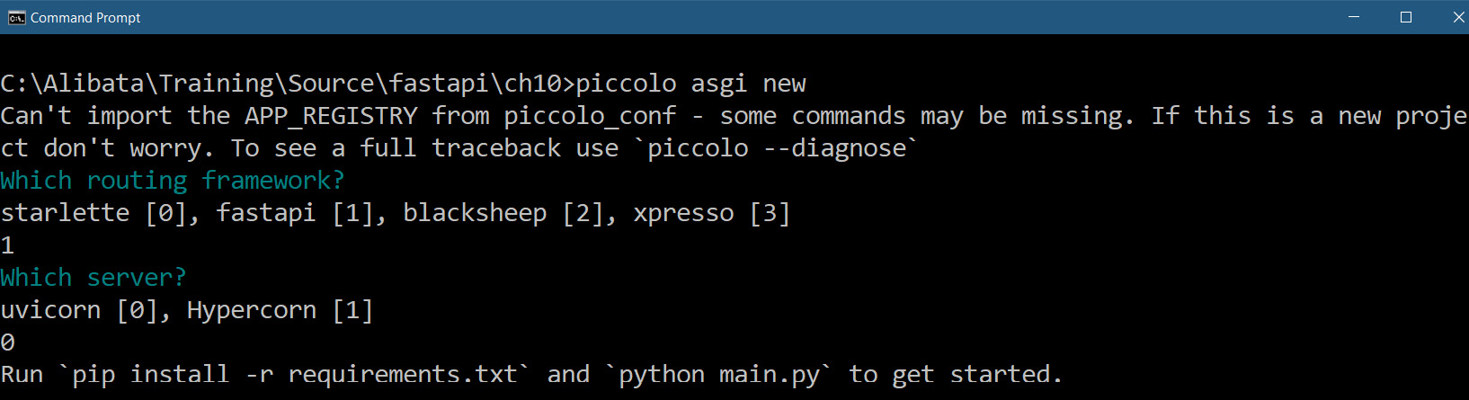
Figure 10.1 – Scaffolding a Piccolo ORM project

You must use FastAPI for the application framework and uvicorn is the recommended ASGI server. Now, we can add Piccolo applications inside the project by running the piccolo app new command inside the project folder. The following screenshot shows the main project directory, where we execute the CLI command to create a Piccolo application:

Figure 10.2 – Piccolo project directory

The scaffolded project always has a default application called home, but it can be modified or even deleted. Once removed, the Piccolo platform allows you to replace home by adding a new application to the project by running the piccolo app new command inside the project folder, as shown in the preceding screenshot. A Piccolo application contains the ORM models, BaseModel, services, repository classes, and API methods. Each application has an auto-generated piccolo_app.py module where we need to configure an APP_CONFIG variable to register all the ORM details. The following is the configuration of our project’s survey application:

APP_CONFIG = AppConfig(
    app_name="survey",
    migrations_folder_path=os.path.join(
        CURRENT_DIRECTORY, "piccolo_migrations"
    ),
    table_classes=[Answers, Education, Question, Choices, 
       Profile, Login, Location, Occupation, Respondent],
    migration_dependencies=[],
    commands=[],
)

For the ORM platform to recognize the new Piccolo application, its piccolo_app.py must be added to APP_REGISTRY of the main project’s piccolo_conf.py module. The following is the content of the piccolo_conf.py file of our ch10-piccolo project:

from piccolo.engine.postgres import PostgresEngine
from piccolo.conf.apps import AppRegistry
DB = PostgresEngine(
    config={
        "database": "pccs",
        "user": "postgres",
        "password": "admin2255",
        "host": "localhost",
        "port": 5433,
    }
)
APP_REGISTRY = AppRegistry(
    apps=["survey.piccolo_app", 
          "piccolo_admin.piccolo_app"]
)

The piccolo_conf.py file is also the module where we establish the PostgreSQL database connection. Aside from PostgreSQL, the Piccolo ORM also supports SQLite databases.

Creating the data models

Like in Django ORM, Piccolo ORM has migration commands to generate the database tables based on model classes. But first, we need to create model classes by utilizing its Table API class. It also has helper classes to establish column mappings and foreign key relationships. The following are some data model classes that comprise our database pccs:

from piccolo.columns import ForeignKey, Integer, Varchar,
       Text, Date, Boolean, Float
from piccolo.table import Table
class Login(Table):
    username = Varchar(unique=True)
    password = Varchar()
class Education(Table):
    name = Varchar()
class Profile(Table):
    fname = Varchar()
    lname = Varchar()
    age = Integer()
    position = Varchar()
    login_id = ForeignKey(Login, unique=True)
    official_id = Integer()
    date_employed = Date()

After creating the model classes, we can update the database by creating the migrations files. Migration is a way of updating the database of a project. In the Piccolo platform, we can run the piccolo migrations new <app_name> command to generate files in the piccolo_migrations folder. These are called migration files and they contain migration scripts. But to save time, we will include the --auto option for the command to let the ORM check the recently executed migration files and auto-generate the migration script containing the newly reflected schema updates. Check the newly created migration file first before running the piccolo migrations forward <app_name> command to execute the migration script. This last command will auto-create all the tables in the database based on the model classes.

Implementing the repository layer

Creating the repository layer comes after performing all the necessary migrations. Piccolo’s CRUD operations are like those in the Peewee ORM. It is swift, short, and easy to implement. The following code shows an implementation of the insert_respondent() transaction, which adds a new respondent profile:

from survey.tables import Respondent
from typing import Dict, List, Any
class RespondentRepository:
    async def insert_respondent(self, 
             details:Dict[str, Any]) -> bool: 
        try:
            respondent = Respondent(**details)
            await respondent.save()
        except Exception as e: 
            return False 
        return True

Like Peewee, Piccolo’s model classes can persist records, as shown by insert_respondent(), which implements an asynchronous INSERT transaction. On the other hand, get_all_respondent() retrieves all respondent profiles and has the same approach as Peewee, as shown here:

    async def get_all_respondent(self):
        return await Respondent.select()
                  .order_by(Respondent.id)

The remaining Peewee-like DELETE and UPDATE respondent transactions are created in the project’s /survey/repository/respondent.py module.

The Beanie ODM

The second version of the PCCS project, ch10-mongo, utilizes a MongoDB datastore and uses the Beanie ODM to implement its asynchronous CRUD transactions. We covered Beanie in Chapter 6, Using a Non-Relational Database. Now, let us learn how to apply FastAPI in symbolic computations. We will be using the ch10-piccolo project for this.

Implementing symbolic computations

Symbolic computation is a mathematical approach to solving problems using symbols or mathematical variables. It uses mathematical equations or expressions formulated using symbolic variables to solve linear and nonlinear systems, rational expressions, logarithmic expressions, and other complex real-world models. To perform symbolic computation in Python, you must install the sympy module using the pip command:

pip install sympy

Let us now start creating our first symbolic expressions.

Creating symbolic expressions

One way of implementing the FastAPI endpoint that performs symbolic computation is to create a service that accepts a mathematical model or equation as a string and converts that string into a sympy symbolic expression. The following substitute_eqn() processes an equation in str format and converts it into valid linear or nonlinear bivariate equations with the x and y variables. It also accepts values for x and y to derive the solution of the expression:

from sympy import symbols, sympify
@router.post("/sym/equation")
async def substitute_bivar_eqn(eqn: str, xval:int, 
               yval:int):
    try:
        x, y = symbols('x, y')
        expr = sympify(eqn)
        return str(expr.subs({x: xval, y: yval}))
    except:
        return JSONResponse(content={"message": 
            "invalid equations"}, status_code=500)

Before converting a string equation into a sympy expression, we need to define the x and y variables as Symbols objects using the symbols() utility. This method accepts a string of comma-delimited variable names and returns a tuple of symbols equivalent to the variables. After creating all the needed Symbols() objects, we can convert our equation into sympy expressions by using any of the following sympy methods:

• sympify(): This uses eval() to convert the string equation into a valid sympy expression with all Python types converted into their sympy equivalents
• parse_expr(): A full-fledged expression parser that transforms and modifies the tokens of the expression and converts them into their sympy equivalents

Since the substitute_bivar_eqn() service utilizes the sympify() method, the string expression needs to be sanitized from unwanted code before sympifying to avoid any compromise.

On the other hand, the sympy expression object has a subs() method to substitute values to derive the solution. Its resulting object must be converted into str format for Response to render the data. Otherwise, Response will raise ValueError, regarding the result as non-iterable.

Solving linear expressions

The sympy module allows you to implement services that solve multivariate systems of linear equations. The following API service highlights an implementation that accepts two bivariate linear models in string format with their respective solutions:

from sympy import Eq, symbols, Poly, solve, sympify
@router.get("/sym/linear")
async def solve_linear_bivar_eqns(eqn1:str, 
            sol1: int, eqn2:str, sol2: int):
    x, y = symbols('x, y')
    
    expr1 = parse_expr(eqn1, locals())
    expr2 = parse_expr(eqn2, locals())
    
    if Poly(expr1, x).is_linear and 
                 Poly(expr1, x).is_linear:
        eq1 = Eq(expr1, sol1)
        eq2 = Eq(expr2, sol2)
        sol = solve([eq1, eq2], [x, y])
        return str(sol)
    else:
        return None

The solve_linear_bivar_eqns() service accepts two bivariate linear equations and their respective outputs (or intercepts) and aims to establish a system of linear equations. First, it registers the x and y variables as sympy objects and then uses the parser_expr() method to transform the string expressions into their sympy equivalents. Afterward, the service needs to establish linear equality of these equations using the Eq() solver, which maps each sympy expression to its solution. Then, the API service passes all these linear equations to the solve() method to derive the x and y values. The result of solve() also needs to be rendered as a string, like in the substitution.

Aside from the solve() method, the API also uses the Poly() utility to create a polynomial object from an expression to be able to access essential properties of an equation, such as is_linear().

Solving non-linear expressions

The previous solve_linear_bivar_eqns() can be reused to solve non-linear systems. The tweak is to shift the validation from filtering the linear equations to any non-linear equations. The following script highlights this code change:

@router.get("/sym/nonlinear")
async def solve_nonlinear_bivar_eqns(eqn1:str, sol1: int, 
           eqn2:str, sol2: int):
    … … … … … …
    … … … … … …    
    if not Poly(expr1, x, y).is_linear or 
              not Poly(expr1, x, y).is_linear:
    … … … … … …
    … … … … … …
        return str(sol)
    else:
        return None

Solving linear and non-linear inequalities

The sympy module supports solving solutions for both linear and non-linear inequalities but on univariate equations only. The following is an API service that accepts a univariate string expression with its output or intercepts, and extracts the solution using the solve() method:

@router.get("/sym/inequality")
async def solve_univar_inequality(eqn:str, sol:int):
    x= symbols('x')
    expr1 = Ge(parse_expr(eqn, locals()), sol)
    sol = solve([expr1], [x])
    return str(sol)

The sympy module has Gt() or StrictGreaterThan, Lt() or StrictLessThan, Ge() or GreaterThan, and Le() or LessThan solvers, which we can use to create inequality. But first, we need to convert the str expression into a Symbols() object using the parser_expr() method before passing them to these solvers. The preceding service uses the GreaterThan solver, which creates an equation where the left-hand side of the expression is generally larger than the left.

Most applications designed and developed for mathematical modeling and data science use sympy to create complex mathematical models symbolically, plot data directly from the sympy equation, or generate results based on datasets or live data. Now, let us proceed to the next group of API services, which deals with data analysis and manipulation using numpy, scipy, and pandas.

Creating arrays and DataFrames

When numerical algorithms require some arrays to store data, a module called NumPy, short for Numerical Python, is a good resource for utility functions, objects, and classes that are used to create, transform, and manipulate arrays.

The module is best known for its n-dimensional arrays or ndarrays, which consume less memory storage than the typical Python lists. An ndarray incurs less overhead when performing data manipulation than executing the list operations in totality. Moreover, ndarray is strictly heterogeneous, unlike Python’s list collections.

But before we start our NumPy-FastAPI service implementation, we need to install the numpy module using the pip command:

pip install numpy

Our first API service will process some survey data and return it in ndarray form. The following get_respondent_answers() API retrieves a list of survey data from PostgreSQL through Piccolo and transforms the list of data into an ndarray:

from survey.repository.answers import AnswerRepository
from survey.repository.location import LocationRepository
import ujson
import numpy as np
@router.get("/answer/respondent")
async def get_respondent_answers(qid:int):
    repo_loc = LocationRepository()
    repo_answers = AnswerRepository()
    locations = await repo_loc.get_all_location()
    data = []
    for loc in locations:
        loc_q = await repo_answers
            .get_answers_per_q(loc["id"], qid)
        if not len(loc_q) == 0:
            loc_data = [ weights[qid-1]
              [str(item["answer_choice"])] 
                for item in loc_q]
            data.append(loc_data)
    arr = np.array(data)
    return ujson.loads(ujson.dumps(arr.tolist())) 

Depending on the size of the data retrieved, it would be faster if we apply the ujson or orjson serializers and de-serializers to convert ndarray into JSON data. Even though numpy has data types such as uint, single, double, short, byte, and long, JSON serializers can still manage to convert them into their standard Python equivalents. Our given API sample prefers ujson utilities to convert the array into a JSON-able response.

Aside from NumPy, pandas is another popular module that’s used in data analysis, manipulation, transformation, and retrieval. But to use pandas, we need to install NumPy, followed by the pandas, matplotlib, and openpxyl modules:

pip install pandas matplotlib openpxyl

Let us now discuss about the ndarray in numpy module.

Applying NumPy’s linear system operations

Data manipulation in an ndarray is easier and faster, unlike in a list collection, which requires list comprehension and loops. The vectors and matrices created by numpy have operations to manipulate their items, such as scalar multiplication, matrix multiplication, transposition, vectorization, and reshaping. The following API service shows how the product between a scalar gradient and an array of survey data is derived using the numpy module:

@router.get("/answer/increase/{gradient}")
async def answers_weight_multiply(gradient:int, qid:int):
    repo_loc = LocationRepository()
    repo_answers = AnswerRepository()
    locations = await repo_loc.get_all_location()
    data = []
    for loc in locations:
        loc_q = await repo_answers
            .get_answers_per_q(loc["id"], qid)
        if not len(loc_q) == 0:
            loc_data = [ weights[qid-1]
             [str(item["answer_choice"])] 
                 for item in loc_q]
            data.append(loc_data)
    arr = np.array(list(itertools.chain(*data)))
    arr = arr * gradient
    return ujson.loads(ujson.dumps(arr.tolist()))

As shown in the previous scripts, all ndarray instances resulting from any numpy operations can be serialized as JSON-able components using various JSON serializers. There are other linear algebraic operations that numpy can implement without sacrificing the performance of the microservice application. Let us take a look now on panda's DataFrame.

Applying the pandas module

In this module, datasets are created as a DataFrame object, similar to in Julia and R. It contains rows and columns of data. FastAPI can render these DataFrames using any JSON serializers. The following API service retrieves all survey results from all survey locations and creates a DataFrame from these datasets:

import ujson
import numpy as np
import pandas as pd
@router.get("/answer/all")
async def get_all_answers():
    repo_loc = LocationRepository()
    repo_answers = AnswerRepository()
    locations = await repo_loc.get_all_location()
    temp = []
    data = []
    for loc in locations:
        for qid in range(1, 13):
            loc_q1 = await repo_answers
               .get_answers_per_q(loc["id"], qid)
            if not len(loc_q1) == 0:
                loc_data = [ weights[qid-1]
                   [str(item["answer_choice"])] 
                      for item in loc_q1]
                temp.append(loc_data)
        temp = list(itertools.chain(*temp))
        if not len(temp) == 0:
            data.append(temp)
        temp = list()
    arr = np.array(data)
    return ujson.loads(pd.DataFrame(arr)
           .to_json(orient='split'))

The DataFrame object has a to_json() utility method, which returns a JSON object with an option to format the resulting JSON according to the desired type. On another note, pandas can also generate time series, a one-dimensional array depicting a column of a DataFrame. Both DataFrames and time series have built-in methods that are useful for adding, removing, updating, and saving the datasets to CSV and XLSX files. But before we discuss pandas’ data transformation processes, let us look at another module that works with numpy in many statistical computations, differentiation, integration, and linear optimizations: the scipy module.

Performing statistical analysis

The scipy module uses numpy as its base module, which is why installing scipy requires numpy to be installed first. We can use the pip command to install the module:

pip install scipy

Our application uses the module to derive the declarative statistics of the survey data. The following get_respondent_answers_stats() API service computes the mean, variance, skewness, and kurtosis of the dataset using the describe() method from scipy:

from scipy import stats
def ConvertPythonInt(o):
    if isinstance(o, np.int32): return int(o)  
    raise TypeError
@router.get("/answer/stats")
async def get_respondent_answers_stats(qid:int):
    repo_loc = LocationRepository()
    repo_answers = AnswerRepository()
    locations = await repo_loc.get_all_location()
    data = []
    for loc in locations:
        loc_q = await repo_answers
           .get_answers_per_q(loc["id"], qid)
             if not len(loc_q) == 0:
                 loc_data = [ weights[qid-1]
                   [str(item["answer_choice"])] 
                       for item in loc_q]
            data.append(loc_data)
    result = stats.describe(list(itertools.chain(*data)))
    return json.dumps(result._asdict(), 
                  default=ConvertPythonInt)

The describe() method returns a DescribeResult object, which contains all the computed results. To render all the statistics as part of Response, we can invoke the as_dict() method of the DescribeResult object and serialize it using the JSON serializer.

Our API sample also uses additional utilities such as the chain() method from itertools to flatten the list of data and a custom converter, ConvertPythonInt, to convert NumPy’s int32 types into Python int types. Now, let us explore how to save data to CSV and XLSX files using the pandas module.

Generating CSV and XLSX reports

The DataFrame object has built-in to_csv() and to_excel() methods that save its data in CSV or XLSX files, respectively. But the main goal is to create an API service that will return these files as responses. The following implementation shows how a FastAPI service can return a CSV file containing a list of respondent profiles:

from fastapi.responses import StreamingResponse
import pandas as pd
from io import StringIO
from survey.repository.respondent import 
        RespondentRepository
@router.get("/respondents/csv", response_description='csv')
async def create_respondent_report_csv():
    repo = RespondentRepository()
    result = await repo.get_all_respondent()
    
    ids = [ item["id"] for item in result ]
    fnames = [ f'{item["fname"]}' for item in result ]
    lnames = [ f'{item["lname"]}' for item in result ]
    ages = [ item["age"] for item in result ]
    genders = [ f'{item["gender"]}' for item in result ]
    maritals = [ f'{item["marital"]}' for item in result ]
   
    dict = {'Id': ids, 'First Name': fnames, 
            'Last Name': lnames, 'Age': ages, 
            'Gender': genders, 'Married?': maritals} 
  
    df = pd.DataFrame(dict)
    outFileAsStr = StringIO()
    df.to_csv(outFileAsStr, index = False)
    return StreamingResponse(
        iter([outFileAsStr.getvalue()]),
        media_type='text/csv',
        headers={
            'Content-Disposition': 
              'attachment;filename=list_respondents.csv',
            'Access-Control-Expose-Headers': 
               'Content-Disposition'
        }
    )

We need to create a dict() containing columns of data from the repository to create a DataFrame object. From the given script, we store each data column in a separate list(), add all the lists in dict() with keys as column header names, and pass dict() as a parameter to the constructor of DataFrame.

After creating the DataFrame object, invoke the to_csv() method to convert its columnar dataset into a text stream, io.StringIO, which supports Unicode characters. Finally, we must render the StringIO object through FastAPI’s StreamResponse with the Content-Disposition header set to rename the default filename of the CSV object.

Instead of using the pandas ExcelWriter, our Online Survey application opted for another way of saving DataFrame through the xlsxwriter module. This module has a Workbook class, which creates a workbook containing worksheets where we can plot all column data per row. The following API service uses this module to render XLSX content:

import xlsxwriter
from io import BytesIO
@router.get("/respondents/xlsx", 
          response_description='xlsx')
async def create_respondent_report_xlsx():
    repo = RespondentRepository()
    result = await repo.get_all_respondent()
    output = BytesIO()
    workbook = xlsxwriter.Workbook(output)
    worksheet = workbook.add_worksheet()
    worksheet.write(0, 0, 'ID')
    worksheet.write(0, 1, 'First Name')
    worksheet.write(0, 2, 'Last Name')
    worksheet.write(0, 3, 'Age')
    worksheet.write(0, 4, 'Gender')
    worksheet.write(0, 5, 'Married?')
    row = 1
    for respondent in result:
        worksheet.write(row, 0, respondent["id"])
        … … … … … …
        worksheet.write(row, 5, respondent["marital"])
        row += 1
    workbook.close()
    output.seek(0)
    headers = {
        'Content-Disposition': 'attachment; 
             filename="list_respondents.xlsx"'
    }
    return StreamingResponse(output, headers=headers)

The given create_respondent_report_xlsx() service retrieves all the respondent records from the database and plots each profile record per row in the worksheet from the newly created Workbook. Instead of writing to a file, Workbook will store its content in a byte stream, io.ByteIO, which will be rendered by StreamResponse.

The pandas module can also help FastAPI services read CSV and XLSX files for rendition or data analysis. It has a read_csv() that reads data from a CSV file and converts it into JSON content. The io.StringIO stream object will contain the full content, including its Unicode characters. The following service retrieves the content of a valid CSV file and returns JSON data:

@router.post("/upload/csv")
async def upload_csv(file: UploadFile = File(...)):
    df = pd.read_csv(StringIO(str(file.file.read(), 
            'utf-8')), encoding='utf-16')
    return orjson.loads(df.to_json(orient='split'))

There are two ways to handle multipart file uploads in FastAPI:

• Use bytes to contain the file
• Use UploadFile to wrap the file object

Chapter 9, Utilizing Other Advanced Features, introduced the UploadFile class for capturing uploaded files because it supports more Pydantic features and has built-in operations that can work with coroutines. It can handle large file uploads without raising an change to - exception when the uploading process reaches the memory limit, unlike using the bytes type for file content storage. Thus, the given read-csv() service uses UploadFile to capture any CSV files for data analysis with orjson as its JSON serializer.

Another way to handle file upload transactions is through Jinja2 form templates. We can use TemplateResponse to pursue file uploading and render the file content using the Jinja2 templating language. The following service reads a CSV file using read_csv() and serializes it into HTML table-formatted content:

@router.get("/upload/survey/form", 
          response_class = HTMLResponse)
def upload_survey_form(request:Request):
    return templates.TemplateResponse("upload_survey.html",
             {"request": request})
@router.post("/upload/survey/form")
async def submit_survey_form(request: Request, 
              file: UploadFile = File(...)):
    df = pd.read_csv(StringIO(str(file.file.read(), 
               'utf-8')), encoding='utf-8')
    return templates.TemplateResponse('render_survey.html', 
         {'request': request, 'data': df.to_html()})

Aside from to_json() and to_html(), the TextFileReader object also has other converters that can help FastAPI render various content types, including to_latex(), to_excel(), to_hdf(), to_dict(), to_pickle(), and to_xarray(). Moreover, the pandas module has a read_excel() that can read XLSX content and convert it into any rendition type, just like its read_csv() counterpart.

Now, let us explore how FastAPI services can plot charts and graphs and output their graphical result through Response.

Plotting data models

With the help of the numpy and pandas modules, FastAPI services can generate and render different types of graphs and charts using the matplotlib utilities. Like in the previous discussions, we will utilize an io.ByteIO stream and StreamResponse to generate graphical results for the API endpoints. The following API service retrieves survey data from the repository, computes the mean for each data strata, and returns a line graph of the data in PNG format:

from io import BytesIO
import matplotlib.pyplot as plt
from survey.repository.answers import AnswerRepository
from survey.repository.location import LocationRepository
@router.get("/answers/line")
async def plot_answers_mean():
    x = [1, 2, 3, 4, 5, 6, 7]
    repo_loc = LocationRepository()
    repo_answers = AnswerRepository()
    locations = await repo_loc.get_all_location()
    temp = []
    data = []
    for loc in locations:
        for qid in range(1, 13):
            loc_q1 = await repo_answers
               .get_answers_per_q(loc["id"], qid)
            if not len(loc_q1) == 0:
                loc_data = [ weights[qid-1]
                  [str(item["answer_choice"])] 
                     for item in loc_q1]
                temp.append(loc_data)
        temp = list(itertools.chain(*temp))
        if not len(temp) == 0:
            data.append(temp)
        temp = list()
    y = list(map(np.mean, data))
    filtered_image = BytesIO()
    plt.figure()
    
    plt.plot(x, y)
 
    plt.xlabel('Question Mean Score')
    plt.ylabel('State/Province')
    plt.title('Linear Plot of Poverty Status')
 
    plt.savefig(filtered_image, format='png')
    filtered_image.seek(0)
   
    return StreamingResponse(filtered_image, 
                media_type="image/png")

The plot_answers_mean() service utilizes the plot() method of the matplotlib module to plot the app’s mean survey results per location on a line graph. Instead of saving the file to the filesystem, the service stores the image in the io.ByteIO stream using the module’s savefig() method. The stream is rendered using StreamResponse, like in the previous samples. The following figure shows the rendered stream image in PNG format through StreamResponse:

Figure 10.3 – Line graph from StreamResponse

The other API services of our app, such as plot_sparse_data(), create a bar chart image in JPEG format of some simulated or derived data:

@router.get("/sparse/bar")
async def plot_sparse_data():
   df = pd.DataFrame(np.random.randint(10, size=(10, 4)),
      columns=["Area 1", "Area 2", "Area 3", "Area 4"])
   filtered_image = BytesIO()
   plt.figure()
   df.sum().plot(kind='barh', color=['red', 'green', 
          'blue', 'indigo', 'violet'])
   plt.title("Respondents in Survey Areas")
   plt.xlabel("Sample Size")
   plt.ylabel("State")
   plt.savefig(filtered_image, format='png')
   
   filtered_image.seek(0)
   return StreamingResponse(filtered_image, 
           media_type="image/jpeg")

The approach is the same as our line graph rendition. With the same strategy, the following service creates a pie chart that shows the percentage of male and female respondents that were surveyed:

@router.get("/respondents/gender")
async def plot_pie_gender():
    repo = RespondentRepository()
    count_male = await repo.list_gender('M')
    count_female = await repo.list_gender('F')
    gender = [len(count_male), len(count_female)]
    filtered_image = BytesIO()
    my_labels = 'Male','Female'
    plt.pie(gender,labels=my_labels,autopct='%1.1f%%')
    plt.title('Gender of Respondents')
    plt.axis('equal')
    plt.savefig(filtered_image, format='png')
    filtered_image.seek(0)
   
    return StreamingResponse(filtered_image, 
               media_type="image/png")

The responses generated by the plot_sparse_data() and plot_pie_gender() services are as follows:

Figure 10.4 – The bar and pie charts generated by StreamResponse

This section will introduce an approach to creating API endpoints that produce graphical results using matplotlib. But there are other descriptive, complex, and stunning graphs and charts that you can create in less time using numpy, pandas, matplotlib, and the FastAPI framework. These extensions can even solve complex mathematical and data science-related problems, given the right hardware resources.

Now, let us shift our focus to the other project, ch10-mongo, to tackle topics regarding workflows, GraphQL, and Neo4j graph database transactions and how FastAPI can utilize them.

Simulating a BPMN workflow

Although the FastAPI framework has no built-in utilities to support its workflows, it is flexible and fluid enough to be integrated into other workflow tools such as Camunda and Apache Airflow through extension modules, middleware, and other customizations. But this section will only focus on the raw solution of simulating BPMN workflows using Celery, which can be extended to a more flexible, real-time, and enterprise-grade approach such as Airflow integration.

Designing the BPMN workflow

The ch10-mongo project has implemented the following BPMN workflow design using Celery:

• A sequence of service tasks that derives the percentage of the survey data result, as shown in the following diagram:

Figure 10.5 – Percentage computation workflow design

• A group of batch operations that saves data to CSV and XLSX files, as shown in the following diagram:

Figure 10.6 – Data archiving workflow design

• A group of chained tasks that operates on each location's data independently, as shown in the following diagram:

Figure 10.7 – Workflow design for stratified survey data analysis

There are many ways to implement the given design, but the most immediate solution is to utilize the Celery setup that we used in Chapter 7, Securing the REST APIs.

Implementing the workflow

Celery’s chain() method implements a workflow of linked task executions, as depicted in Figure 10.5, where every parent task returns the result to the first parameter of next task. The chained workflow works if each task runs successfully without encountering any exceptions at runtime. The following is the API service in /api/survey_workflow.py that implements the chained workflow:

@router.post("/survey/compute/avg")
async def chained_workflow(surveydata: SurveyDataResult):
    survey_dict = surveydata.dict(exclude_unset=True)
    result = chain(compute_sum_results
        .s(survey_dict['results']).set(queue='default'), 
            compute_avg_results.s(len(survey_dict))
             .set(queue='default'), derive_percentile.s()
             .set(queue='default')).apply_async()
    return {'message' : result.get(timeout = 10) }

compute_sum_results(), compute_avg_results(), and derive_percentile() are bound tasks. Bound tasks are Celery tasks that are implemented to have the first method parameter allocated to the task instance itself, thus the self keyword appearing in its parameter list. Their task implementation always has the @celery.task(bind=True) decorator. The Celery task manager prefers bound tasks when applying workflow primitive signatures to create workflows. The following code shows the bound tasks that are used in the chained workflow design:

@celery.task(bind=True)
def compute_sum_results(self, results:Dict[str, int]):
    scores = []
    for key, val in results.items():
        scores.append(val)
    return sum(scores)

compute_sum_results() computes the total survey result per state, while compute_avg_results()consumes the sum computed by compute_sum_results() to derive the mean value:

@celery.task(bind=True)
def compute_avg_results(self, value, len):
    return (value/len)

On the other hand, derive_percentile() consumes the mean values produced by compute_avg_results() to return a percentage value:

@celery.task(bind=True)
def derive_percentile(self, avg):
    percentage = f"{avg:.0%}"
    return percentage

The given derive_percentile() consumes the mean values produced by compute_avg_results() to return a percentage value.

To implement the gateway approach, Celery has a group() primitive signature, which is used to implement parallel task executions, as depicted in Figure 10.6. The following API shows the implementation of the workflow structure with parallel executions:

@router.post("/survey/save")
async def grouped_workflow(surveydata: SurveyDataResult):
    survey_dict = surveydata.dict(exclude_unset=True)
    result = group([save_result_xlsx
       .s(survey_dict['results']).set(queue='default'), 
         save_result_csv.s(len(survey_dict))
          .set(queue='default')]).apply_async()
    return {'message' : result.get(timeout = 10) } 

The workflow shown in Figure 10.7 depicts a mix of grouped and chained workflows. It is common for many real-world microservice applications to solve workflow-related problems with a mixture of different Celery signatures, including chord(), map(), and starmap(). The following script implements a workflow with mixed signatures:

@router.post("/process/surveys")
async def process_surveys(surveys: List[SurveyDataResult]):
    surveys_dict = [s.dict(exclude_unset=True) 
         for s in surveys]
    result = group([chain(compute_sum_results
       .s(survey['results']).set(queue='default'), 
         compute_avg_results.s(len(survey['results']))
         .set(queue='default'), derive_percentile.s()
         .set(queue='default')) for survey in 
                surveys_dict]).apply_async()
    return {'message': result.get(timeout = 10) }

The Celery signature plays an essential role in building workflows. A signature() method or s() that appears in the construct manages the execution of the task, which includes accepting the initial task parameter value(s) and utilizing the queues that the Celery worker uses to load tasks. As discussed in Chapter 7, Securing the REST APIs, apply_async() triggers the whole workflow execution and retrieves the result.

Aside from workflows, the FastAPI framework can also use the GraphQL platform to build CRUD transactions, especially when dealing with a large amount of data in a microservice architecture.

Using GraphQL queries and mutations

GraphQL is an API standard that implements REST and CRUD transactions at the same time. It is a high-performing platform that’s used in building REST API endpoints that only need a few steps to set up. Its objective is to create endpoints for data manipulation and query transactions.

Setting up the GraphQL platform

Python extensions such as Strawberry, Ariadne, Tartiflette, and Graphene support GraphQL-FastAPI integration. This chapter introduces the use of the new Ariadne 3.x to build CRUD transactions for this ch10-mongo project with MongoDB as the repository.

First, we need to install the latest graphene extension using the pip command:

pip install graphene

Among the GraphQL libraries, Graphene is the easiest to set up, with fewer decorators and methods to override. It easily integrates with the FastAPI framework without requiring additional middleware and too much auto-wiring.

Creating the record insertion, update, and deletion

Data manipulation operations are always part of GraphQL’s mutation mechanism. This is a GraphQL feature that modifies the server-side state of the application and returns arbitrary data as a sign of a successful change in the state. The following is an implementation of a GraphQL mutation that inserts, deletes, and updates records:

from models.data.pccs_graphql import LoginData
from graphene import String, Int, Mutation, Field
from repository.login import LoginRepository
class CreateLoginData(Mutation):
    class Arguments:
      id = Int(required=True)
      username = String(required=True)
      password = String(required=True)
    ok = Boolean()
    loginData = Field(lambda: LoginData)
    async def mutate(root, info, id, username, password):
        login_dict = {"id": id, "username": username, 
                   "password": password}
        login_json = dumps(login_dict, default=json_serial)
        repo = LoginRepository()
        result = await repo.add_login(loads(login_json))
        if not result == None:
          ok = True
        else: 
          ok = False
        return CreateLoginData(loginData=result, ok=ok)

CreateLoginData is a mutation that adds a new login record to the data store. The inner class, Arguments, indicates the record fields that will comprise the new login record for insertion. These arguments must appear in the overridden mutate() method to capture the values of these fields. This method will also call the ORM, which will persist the newly created record.

After a successful insert transaction, mutate() must return the class variables defined inside a mutation class such as ok and the loginData object. These returned values must be part of the mutation instance.

Updating a login attribute has a similar implementation to CreateLoginData except the arguments need to be exposed. The following is a mutation class that updates the password field of a login record that’s been retrieved using its username:

class ChangeLoginPassword(Mutation):
    class Arguments:
      username = String(required=True)
      password = String(required=True)
    ok = Boolean()
    loginData = Field(lambda: LoginData)
    async def mutate(root, info, username, password):       
        repo = LoginRepository()
        result = await repo.change_password(username, 
                  password)
        
        if not result == None:
          ok = True
        else: 
          ok = False
        return CreateLoginData(loginData=result, ok=ok)

Similarly, the delete mutation class retrieves a record through an id and deletes it from the data store:

class DeleteLoginData(Mutation):
    class Arguments:
      id = Int(required=True)
      
    ok = Boolean()
    loginData = Field(lambda: LoginData)
    async def mutate(root, info, id):       
        repo = LoginRepository()
        result = await repo.delete_login(id)
        if not result == None:
          ok = True
        else: 
          ok = False
        return DeleteLoginData(loginData=result, ok=ok)

Now, we can store all our mutation classes in an ObjectType class that exposes these transactions to the client. We assign field names to each Field instance of the given mutation classes. These field names will serve as the query names of the transactions. The following code shows the ObjectType class, which defines our CreateLoginData, ChangeLoginPassword, and DeleteLoginData mutations:

class LoginMutations(ObjectType):
    create_login = CreateLoginData.Field()
    edit_login = ChangeLoginPassword.Field()
    delete_login = DeleteLoginData.Field()

Implementing the query transactions

GraphQL query transactions are implementations of the ObjectType base class. Here, LoginQuery retrieves all login records from the data store:

class LoginQuery(ObjectType):
    login_list = None
    get_login = Field(List(LoginData))
  
    async def resolve_get_login(self, info):
      repo = LoginRepository()
      login_list = await repo.get_all_login()
      return login_list

The class must have a query field name, such as get_login, that will serve as its query name during query execution. The field name must be part of the resolve_*() method name for it to be registered under the ObjectType class. A class variable, such as login_list, must be declared for it to contain all the retrieved records.

Running the CRUD transactions

We need a GraphQL schema to integrate the GraphQL components and register the mutation and query classes for the FastAPI framework before running the GraphQL transactions. The following script shows the instantiation of GraphQL’s Schema class with LoginQuery and LoginMutations:

from graphene import Schema 
schema = Schema(query=LoginQuery, mutation=LoginMutations,
    auto_camelcase=False)

We set the auto_camelcase property of the Schema instance to False to maintain the use of the original field names with an underscore and avoid the camel case notation approach.

Afterward, we use the schema instance to create the GraphQLApp() instance. GraphQLApp is equivalent to an application that needs mounting to the FastAPI framework. We can use the mount() utility of FastAPI to integrate the GraphQLApp() instance with its URL pattern and the chosen GraphQL browser tool to run the API transactions. The following code shows how to integrate the GraphQL applications with Playground as the browser tool to run the APIs:

from starlette_graphene3 import GraphQLApp,     
          make_playground_handler
app = FastAPI()
app.mount("/ch10/graphql/login", 
       GraphQLApp(survey_graphene_login.schema, 
          on_get=make_playground_handler()) )
app.mount("/ch10/graphql/profile", 
       GraphQLApp(survey_graphene_profile.schema, 
          on_get=make_playground_handler()) )

We can use the left-hand side panel to insert a new record through a JSON script containing the field name of the CreateLoginData mutation, which is create_login, along with passing the necessary record data, as shown in the following screenshot:

Figure 10.8 – Running the create_login mutation

To perform query transactions, we must create a JSON script with a field name of LoginQuery, which is get_login, together with the record fields needed to be retrieved. The following screenshot shows how to run the LoginQuery transaction:

Figure 10.9 – Running the get_login query transaction

GraphQL can help consolidate all the CRUD transactions from different microservices with easy setup and configuration. It can serve as an API Gateway where all GraphQLApps from multiple microservices are mounted to create a single façade application. Now, let us integrate FastAPI into a graph database.

Utilizing the Neo4j graph database

For an application that requires storage that emphasizes relationships among data records, a graph database is an appropriate storage method to use. One of the platforms that use graph databases is Neo4j. FastAPI can easily integrate with Neo4j, but we need to install the Neo4j module using the pip command:

pip install neo4j

Neo4j is a NoSQL database with a flexible and powerful data model that can manage and connect different enterprise-related data based on related attributes. It has a semi-structured database architecture with simple ACID properties and a non-JOIN policy that make its operations fast and easy to execute.

Note

ACID, which stands for atomicity, consistency, isolation, and durability, describes a database transaction as a group of operations that performs as a single unit with correctness and consistency.

Setting the Neo4j database

The neo4j module includes neo4j-driver, which is needed to establish a connection with the graph database. It needs a URI that contains the bolt protocol, server address, and port. The default database port to use is 7687. The following script shows how to create Neo4j database connectivity:

from neo4j import GraphDatabase
uri = "bolt://127.0.0.1:7687"
driver = GraphDatabase.driver(uri, auth=("neo4j", 
      "admin2255"))

Creating the CRUD transactions

Neo4j has a declarative graph query language called Cypher that allows CRUD transactions of the graph database. These Cypher scripts need to be encoded as str SQL commands to be executed by its query runner. The following API service adds a new database record to the graph database:

@router.post("/neo4j/location/add")
def create_survey_loc(node_name: str, 
        node_req_atts: LocationReq):
    node_attributes_dict = 
          node_req_atts.dict(exclude_unset=True)
    node_attributes = '{' + ', '.join(f'{key}:'{value}''
        for (key, value) in node_attributes_dict.items()) 
              + '}'
    query = f"CREATE ({node_name}:Location  
         {node_attributes})"
    try:
        with driver.session() as session:
            session.run(query=query)
        return JSONResponse(content={"message":
         "add node location successful"}, status_code=201)
    except Exception as e:
        print(e)
        return JSONResponse(content={"message": "add node 
            location unsuccessful"}, status_code=500)

create_survey_loc() adds new survey location details to the Neo4j database. A record is considered a node in the graph database with a name and attributes equivalent to the record fields in the relational databases. We use the connection object to create a session that has a run() method to execute Cypher scripts.

The command to add a new node is CREATE, while the syntax to update, delete, and retrieve nodes can be added with the MATCH command. The following update_node_loc() service searches for a particular node based on the node’s name and performs the SET command to update the given fields:

@router.patch("/neo4j/update/location/{id}")
async def update_node_loc(id:int, 
           node_req_atts: LocationReq):
    node_attributes_dict = 
         node_req_atts.dict(exclude_unset=True)
    node_attributes = '{' + ', '.join(f'{key}:'{value}'' 
       for (key, value) in 
            node_attributes_dict.items()) + '}'
    query = f"""
        MATCH (location:Location)
        WHERE ID(location) = {id}
        SET location += {node_attributes}"""
    try:
        with driver.session() as session:
            session.run(query=query)
        return JSONResponse(content={"message": 
          "update location successful"}, status_code=201)
    except Exception as e:
        print(e)
        return JSONResponse(content={"message": "update 
           location  unsuccessful"}, status_code=500)

Likewise, the delete transaction uses the MATCH command to search for the node to be deleted. The following service implements Location node deletion:

@router.delete("/neo4j/delete/location/{node}")
def delete_location_node(node:str):
    node_attributes = '{' + f"name:'{node}'" + '}'
    query = f"""
        MATCH (n:Location {node_attributes})
        DETACH DELETE n
    """
    try:
        with driver.session() as session:
            session.run(query=query)
        return JSONResponse(content={"message": 
          "delete location node successful"}, 
             status_code=201)
    except:
        return JSONResponse(content={"message": 
           "delete location node unsuccessful"}, 
               status_code=500)

When retrieving nodes, the following service retrieves all the nodes from the database:

@router.get("/neo4j/nodes/all")
async def list_all_nodes():
    query = f"""
        MATCH (node)
        RETURN node"""
    try:
        with driver.session() as session:
            result = session.run(query=query)
            nodes = result.data()
        return nodes
    except Exception as e:
        return JSONResponse(content={"message": "listing
            all nodes unsuccessful"}, status_code=500)

The following service only retrieves a single node based on the node’s id:

@router.get("/neo4j/location/{id}")
async def get_location(id:int):
    query = f"""
        MATCH (node:Location)
        WHERE ID(node) = {id}
        RETURN node"""
    try:
        with driver.session() as session:
            result = session.run(query=query)
            nodes = result.data()
        return nodes
    except Exception as e:
        return JSONResponse(content={"message": "get 
          location node unsuccessful"}, status_code=500)

Our implementation will not be complete if we have no API endpoint that will link nodes based on attributes. Nodes are linked to each other based on relationship names and attributes that are updatable and removable. The following API endpoint creates a node relationship between the Location nodes and Respondent nodes:

@router.post("/neo4j/link/respondent/loc")
def link_respondent_loc(respondent_node: str, 
    loc_node: str, node_req_atts:LinkRespondentLoc):
    node_attributes_dict = 
         node_req_atts.dict(exclude_unset=True)
   
    node_attributes = '{' + ', '.join(f'{key}:'{value}'' 
       for (key, value) in 
          node_attributes_dict.items()) + '}'
  
    query = f"""
        MATCH (respondent:Respondent), (loc:Location)
        WHERE respondent.name = '{respondent_node}' AND 
            loc.name = '{loc_node}'
        CREATE (respondent) -[relationship:LIVES_IN 
              {node_attributes}]->(loc)"""
    try:
        with driver.session() as session:
            session.run(query=query)
        return JSONResponse(content={"message": "add … 
            relationship successful"}, status_code=201)
    except:
        return JSONResponse(content={"message": "add 
          respondent-loc relationship unsuccessful"}, 
                 status_code=500)

The FastAPI framework can easily integrate into any database platform. The previous chapters have proven that FastAPI can deal with relational database transactions with ORM and document-based NoSQL transactions with ODM, while this chapter has proven the same for the Neo4j graph database due to its easy configurations.

Summary

This chapter introduced the scientific side of FastAPI by showing that API services can provide numerical computation, symbolic formulation, and graphical interpretation of data via the numpy, pandas, sympy, and matplotlib modules. This chapter also helped us understand how far we can integrate FastAPI with new technology and design strategies to provide new ideas for the microservice architecture, such as using GraphQL to manage CRUD transactions and Neo4j for real-time and node-based data management. We also introduced the basic approach that FastAPI can apply to solve various BPMN workflows using Celery tasks. With this, we have started to understand the power and flexibility of the framework in building microservice applications.

The next chapter will cover the last set of topics to complete our deep dive into FastAPI. We will cover some deployment strategies, Django and Flask integrations, and other microservice design patterns that haven’t been discussed in the previous chapters.