
Chapter 12
Analysis of Variance and Experimental Designs
Learning Objectives
Upon completion of this chapter, you will be able to:
- Understand the concept of ANOVA and experimental designs
- Compute and interpret the result of completely randomized design (one-way ANOVA)
- Understand Post Hoc Comparisons in ANOVA
- Compute and interpret the result of randomized block design
- Compute and interpret the result of factorial design (two-way ANOVA)
- Understand basics of three-way ANOVA and MANOVA
Statistics in Action: Tata Motors Ltd
Tata Motors Ltd, widely known as TELCO, established in 1945, is one of India’s oldest automobile manufacturing companies. It is the leader in commercial vehicles in each segment, and is one among the top three in the passenger vehicles market with winning products in the compact, midsize car, and utility-vehicles segments. The company is the world’s fourth largest truck manufacturer and the world’s second largest bus manufacturer.1
Tata Motors acquired the Daewoo Commercial Vehicles Company, South Korea’s second largest truck maker, in 2004. The next year, it acquired a 21% stake in Hispano Carrocera, a reputed Spanish bus and coach manufacturer, with an option to acquire the remaining stake as well. In 2006, the company entered into a joint venture with the Brazil-based Marcopolo. In the same year it also entered into a joint venture with the Thonburi Automotive Assembly Plant Company of Thailand to manufacture and market the company’s pick-up vehicles in Thailand.1 Table 12.1 shows the profit after tax of the company from 1995 to 2007.
Table 12.1 Profit after tax of Tata Motors Ltd from 1995–2007 (in million rupees)

Source: Prowess (V. 3.1), Centre for Monitoring Indian Economy Pvt. Ltd, Mumbai accessed August 2008, reproduced with permission.
Tata Motors unveiled “Tata Nano,” a Rs one-lakh car (excluding VAT and transportation costs) in January 2008. The Tata Nano is expected to shift thousands of two-wheeler owners into car owners because of its affordable price. The market segmentation of the passenger car segment by region is as shown in Table 12.2.
Table 12.2 Region wise market share of passenger cars

Source: www.indiastat.com, accessed August 2008, reproduced with permission.
Suppose Tata Motors wants to ascertain the purchase behaviour of the future consumers of Tata Nano in four segments of the country. The company has used a questionnaire consisting of 10 questions and used a 5-point rating scale with 1 as ‘strongly disagree’ and 5 as ‘strongly agree’. It has taken a random sample of 3000 potential customers from each region with the objective of finding out the difference in the mean scores of each region. In order to find out the significant mean difference of potential consumer purchase behaviour in the four regions taken for the study, the company can analyse the data adopting a statistical technique commonly known as ANOVA. This chapter focuses on the concept of ANOVA and experimental designs; completely randomized design (one-way ANOVA); randomized block design, and factorial design (two-way ANOVA).
12.1 Introduction
In the previous chapter, we discussed the various techniques of analysing data from two samples (taken from two populations). These techniques were related to means and proportions. In real life, there may be situations when instead of comparing two sample means, a researcher has to compare three or more than three sample means (specifically, more than two). A researcher may have to test whether the three or more sample means computed from the three populations are equal. In other words, the null hypothesis can be, that three or more population means are equal as against the alternative hypothesis that these population means are not equal. For example, suppose that a researcher wants to measure work attitude of the employees in four organizations. The researcher has prepared a questionnaire consisting of 10 questions for measuring the work attitude of employees. A five-point rating scale is used with 1 being the lowest score and 5 being the highest score. So, an employee can score 10 as the minimum score and 50 as the maximum score. The null hypothesis can be set as all the means are equal (there is no difference in the degree of work attitude of the employees) as against the alternative hypothesis that at least one of the means is different from the others (there is a significant difference in the degree of work attitude of the employees).
12.2 Introduction to Experimental Designs
An experimental design is the logical construction of an experiment to test hypothesis in which the researcher either controls or manipulates one or more variables. Some of the widely used terms while discussing experimental designs are as follows:
An experimental design is the logical construction of an experiment to test hypothesis in which the researcher either controls or manipulates one or more variables.
Independent variable: In an experimental design, the independent variable may be either a treatment variable or a classification variable.
Treatment variable: This is a variable which is controlled or modified by the researcher in the experiment. For example, in agriculture, the different fertilizers or the different methods of cultivation are the treatments.
Classification variable: Classification variable can be defined as the characteristics of the experimental subject that are present prior to the experiment and not a result of the researcher’s manipulation or control.
Experimental Units: The smallest division of the experimental material to which treatments are applied and observations are made are referred to as experimental units.
Dependent variable: In experimental design, a dependent variable is the response to the different levels of independent variables. This is also called response variable.
Factor: A factor can be referred to as a set of treatments of a single type. In most situations, a researcher may be interested in studying more than one factor. For example, a researcher in the field of advertising may be interested in studying the impact of colour and size of advertisements on consumers. In addition, the researcher may be interested in knowing the difference in average responses to three different colours and four different sizes of the advertisement. This is referred to as two-factor ANOVA.
12.3 Analysis of Variance
Analysis of variance or ANOVA is a technique of testing hypotheses about the significant difference in several population means. This technique was developed by R. A. Fisher. In this chapter, experimental designs will be analysed by using ANOVA. The main purpose of analysis of variance is to detect the difference among various population means based on the information gathered from the samples (sample means) of the respective populations.
Analysis of variance or ANOVA is a technique of testing hypotheses about the significant difference in several population means.
Analysis of variance is also based on some assumptions. Each population should have a normal distribution with equal variances. For example, if there are n populations, variances of each population, that is, ![]() Each sample taken from the population should be randomly drawn and should be independent of each other.
Each sample taken from the population should be randomly drawn and should be independent of each other.
In analysis of variance, the total variation in the sample data can be on account of two components, namely, variance between the samples and variance within the samples. Variance between samples is attributed to the difference among the sample means. This variance is due to some assignable causes. Variance within the samples is the difference due to chance or experimental errors. For the sake of clarity, the techniques of analysis of variance can be broadly classified into one-way classification and two-way classification. In fact, many different types of experimental designs are available to the researchers. This chapter will focus on three specific types of experimental designs, namely, completely randomized design, randomized block design, and factorial design. ANOVA is based on the following assumptions:
In analysis of variance, the total variation in the sample data can be on account of two components, namely, variance between the samples and variance within the samples. Variance between the samples is attributed to the difference among the sample means. This variance is due to some assignable causes. Variance within the samples is the difference due to chance or experimental errors.
- Dependent variable must be metric.
- Independent variables should have two or more categories or independent groups.
- Significant outliers should not be present.
- Samples are being drawn from a normally distributed population.
- Samples are randomly drawn from the population and are independent of each other.
- Dependent variable should be approximately normally distributed for combination of groups of independent variables.
- Population from which samples are being drawn should have equal variances. This assumption is referred to as homogeneity of variances.
12.4 Completely randomized design (One-way ANOVA)
Completely randomized design contains only one independent variable, with two or more treatment levels or classifications. In case of only two treatment levels or classifications, the design would be the same as that used for hypothesis testing for two populations in Chapter 11. When there is a case of three or more classification levels, analysis of variance is used to analyse the data.
Completely randomized design contains only one independent variable, with two or more treatment levels or classifications.
Suppose a researcher wants to test the stress level of employees in three different organizations. For conducting this research, he has prepared a questionnaire with a five-point rating scale with 1 being the minimum score and 5 being the maximum score. The researcher has administered the questionnaire and obtained the mean score for three organizations. The researcher could have used the z-test or t test for two populations if there had been only two populations. In this case, there are three populations, so there is no scope of using z-test or t test for testing the hypotheses. In this case, one-way analysis of variance technique can be effectively used to analyse the data. One-way analysis of variance can also be used very effectively in the case of comparison among sample means taken from more than two populations One-way is used since there is only one independent variable.1
Suppose if k samples are being analysed by a researcher, then the null and alternative hypotheses can be set as below:
In one-way analysis of variance, testing of hypothesis can be carried out by partitioning the total variation of the data in two parts. The first part is the variance between the samples and the second part is the variance within the samples. The variance between the samples can be attributed to treatment effects and variance within the samples can be attributed to experimental errors.
H0: μ1 = μ2=μ3= … =μk
The alternative hypothesis can be set as below:
H1: Not all μjs are equal (j = 1, 2, 3, …, k)
The null hypothesis indicates that all population means for all levels of treatments are equal. If one population mean is different from another, the null hypothesis is rejected and the alternative hypothesis is accepted.
In one-way analysis of variance, testing of hypothesis is carried out by partitioning the total variation of the data in two parts. The first part is the variance between the samples and the second part is the variance within the samples. The variance between the samples can be attributed to treatment effects and variance within the samples can be attributed to experimental errors. As part of this process, the total sum of squares can be divided into two additive and independent parts as shown in Figure 12.1:
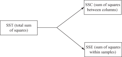
Figure 12.1 Partitioning the total sum of squares of the variation for completely randomized design (one-way ANOVA)
SST (total sum of squares) = SSC (sum of squares between columns) + SSE (sum of squares within samples)
12.4.1 Steps in Calculating SST (Total Sum of Squares) and Mean Squares in One-Way Analysis of Variance
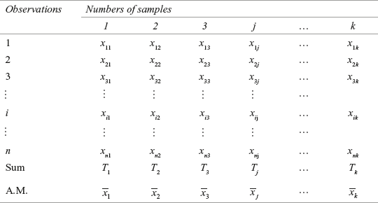
As discussed above, the total sum of squares can be partitioned in two parts: sum of squares between columns and sum of squares within samples. So, there are two steps in calculating SST (total sum of squares) in one-way analysis of variance, in terms of calculating sum of squares between columns and sum of squares within samples. Let us say that the observations obtained for k independent samples is based on one-criterion classification and can be arranged as shown in the Table 12.3 below:
Table 12.3 Observations obtained for k independent samples based on one-criterion classification
The variance between columns measures the difference between the sample mean of each group and the grand mean. The grand mean is the overall mean and can be obtained by adding all the individual observations of the columns and then dividing this total by the number of total observations.
where ![]()
![]() and
and ![]()
- 1. Calculate variance between columns (samples): This is usually referred to as sum of squares between samples and is usually denoted by SSC. The variance between columns measures the difference between the sample mean of each group and the grand mean. Grand mean is the overall mean and can be obtained by adding all the individual observations of the columns and then dividing this total by the total number of observations. The procedure of calculating the variance between the samples is as below:
- (a) In the first step, we need to calculate the mean of each sample. From Table 12.3, the means are

- (b) Next, the grand mean is calculated. The grand mean is calculated as

- (c) In Step 3, the difference between the mean of each sample and grand mean is calculated, that is, we calculate
 .
. - (d) In Step 4, we multiply each of these by the number of observations in the corresponding sample, square each of these deviations and add them. This will give the sum of the squares between samples.
- (e) In the last step, the total obtained in Step 4 is divided by the degrees of freedom. The degrees of freedom is one less than the total number of samples. If there are k samples, the degrees of freedom will be v = k – 1. When the sum of squares obtained in Step 4 is divided by the number of degrees of freedom, the result is called mean square (MSC) and is an alternative term for sample variance.
SSC (sum of squares between columns) =

where k is the number of groups being compared, nj the number of observations in Group j,
 the sample mean of Group j, and
  the grand mean.
 and MSC (mean square) =

where SSC is the sum of squares between columns and k – 1 the degrees of freedom (number of samples – 1).
- (a) In the first step, we need to calculate the mean of each sample. From Table 12.3, the means are
- 2. Calculate variance within columns (samples): This is usually referred to as the sum of squares within samples. The variance within columns (samples) measures the difference within the samples (intra-sample difference) due to chance. This is usually denoted by SSE. The procedure of calculating the variance within the samples is as below:
The variance within columns (samples) measures the difference within the samples (intra-sample difference) due to chance. This is usually denoted by SSE.
- (a) In calculating the variance within samples, the first step is to calculate the mean of each sample. From Table 12.3 this is

- (b) Second step is to calculate the deviation of each observation in k samples from the mean values of the respective samples.
- (c) As a third step, square all the deviations obtained in Step 2 and calculate the total of all these squared deviations.
- (d) As the last step, divide the total squared deviations obtained in Step 3 by the degrees of freedom and obtain the mean square. The number of degrees of freedom can be calculated as the difference between the total number of observations and the number of samples. If there are n observations and k samples then the degrees of freedom is v = n – k
SSE (sum of squares within samples) =

where xij is the ith observation in Group j,
 the sample mean of Group j, k the number of groups being compared, and n the total number of observations in all the groups.
and MSE (mean square) =

where SSE is the sum of squares within columns and n – k the degrees of freedom (total number of observations – number of samples).
- (a) In calculating the variance within samples, the first step is to calculate the mean of each sample. From Table 12.3 this is
- 3. Calculate total sum of squares: The total variation is equal to the sum of the squared difference between each observation (sample value) and the grand mean
 . This is often referred to as SST (total sum of squares). So, the total sum of squares can be calculated as below:
The total variation is equal to the sum of the difference between each observation (sample value) and the grand mean
 This is often referred to as SST (total sum of squares).
SST (total sum of squares) = SSC (sum of squares between columns) + SSE (sum of squares within samples)

SST (total sum of squares) =

where xij is the ith observation in Group j,
 the grand mean, k the number of groups being compared, and n the total number of observations in all the groups
and MST (mean square) =

where SST is the total sum of squares and
n – 1 the degrees of freedom (number of observations – 1).
12.4.2 Applying the F-Test Statistic
As discussed, ANOVA can be computed with three sums of squares: SSC (sum of squares between columns), SSE (sum of squares within samples), and SST (total sum of squares). As discussed in the previous chapter (Chapter 11), F is the ratio of two variances. In case of ANOVA, F value is obtained by dividing the treatment variance (MSC) by the error variance (MSE). So, in case of ANOVA, F value is calculated as below:
In case of ANOVA, F value is obtained by dividing the treatment variance (MSC) by the error variance (MSE).
F test statistic in one-way ANOVA
![]()
where MSC is the mean square column and MSE the mean square error.
The F test statistic follows F distribution with k – 1 degrees of freedom corresponding to MSC in the numerator and n – k degrees of freedom corresponding to MSE in the denominator. The null hypothesis is rejected if the calculated value of F is greater than the upper-tail critical value FU with k – 1 degrees of freedom in the numerator and n – k degrees of freedom in the denominator. For a given level of significance α, the rules for acceptance or rejection of the null hypothesis are shown below:
For a given level of significance α, the rules for acceptance or rejection of the null hypothesis
Reject H0, if calculated F > FU (Upper tail value of F),
otherwise do not reject H0.
Figure 12.2 exhibits the rejection and non-rejection region (acceptance region) when using ANOVA to test the null hypothesis.

Figure 12.2 Rejection and non-rejection region (acceptance region) when using ANOVA to test null hypothesis
12.4.3 The ANOVA Summary Table
The result of ANOVA is usually presented in an ANOVA table (shown in Table 12.4). The entries in the table consist of SSC (sum of squares between columns), SSE (sum of squares within samples) and SST(total sum of squares); corresponding degrees of freedom k – 1, n – k and, n – 1; MSC (mean square column) and MSE (mean square error); and F value. The ANOVA summary table is not always included in the body of a research paper but it is a valuable source of information about the result of the analysis.2 When using software programs such as MS Excel, Minitab, and SPSS, the summary table also includes the p value. The p value allows a researcher to make inferences directly without taking help from the critical values of the F distribution.
Table 12.4 ANOVA Summary Table

Example 12.1
Vishal Foods Ltd is a leading manufacturer of biscuits. The company has launched a new brand in the four metros; Delhi, Mumbai, Kolkata, and Chennai. After one month, the company realizes that there is a difference in the retail price per pack of biscuits across cities. Before the launch, the company had promised its employees and newly-appointed retailers that the biscuits would be sold at a uniform price in the country. The difference in price can tarnish the image of the company. In order to make a quick inference, the company collected data about the price from six randomly selected stores across the four cities. Based on the sample information, the price per pack of the biscuits (in rupees) is given in Table 12.5:
TABLE 12.5 Price per pack of the biscuits (in rupees)
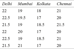
Use one-way ANOVA to analyse the significant difference in the prices. Take 95% as the confidence level.
Solution The seven steps of hypothesis testing can be performed as below:
Step 1: Set null and alternative hypotheses
The null and alternative hypothesis can be stated as below:
![]()
and H1: All the means are not equal
Step 2: Determine the appropriate statistical test
The appropriate test statistic is F test statistic in one-way ANOVA given as below
![]()
where MSC = mean square column
MSE = mean square error
Step 3: Set the level of significance
Alpha has been specified as 0.05.
Step 4: Set the decision rule
For a given level of significance 0.05, the rules for acceptance or rejection of null hypothesis are as follows:
Reject H0 if calculated F > FU (upper-tail value of F),
otherwise, do not reject H0.
In this problem, for the numerator and the denominator the degrees of freedom are 3 and 20 respectively. The critical F-value is F0.05, 3, 20 = 3.10.
Step 5: Collect the sample data
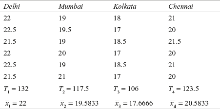
The sample data is as shown in Table 12.6.
Table 12.6 Sample data for Example 12.1
Step 6: Analyse the data
From the table
![]() ;
;
![]()
and n1 = n2 = n3 = n4 = 6
SSC (sum of squares between columns) = ![]()

= 25.0104 + 0.8437 + 31.5104 + 2.3437 = 59.7083
SSE (sum of squares within samples) =![]()
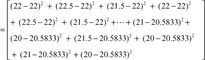
= 9.25
SST (total sum of squares) = ![]()

= 68.9583
MSC (mean square) = ![]()
MSE (mean square) = ![]()
![]()
Figure 12.7 exhibits the ANOVA table for Example 12.1
Table 12.7 ANOVA table for Example 12.1

Step 7: Arrive at a statistical conclusion and business implication
At 95% confidence level, the critical value obtained from the F table is F0.05, 3, 20 = 3.10. The calculated value of F is 43.03, which is greater than the tabular value (critical value) and falls in the rejection region. Hence, the null hypothesis is rejected and the alternative hypothesis is accepted.
There is enough evidence to believe that there is a significant difference in the prices across four cities. So, the management must initiate corrective steps to ensure that the prices should remain uniform. This must be done urgently to protect the credibility of the firm.
12.4.4 Using MS Excel for Hypothesis Testing with the F Statistic for the Difference in Means of More Than Two Populations
MS Excel can be used for hypothesis testing with F statistic for difference in means of more than two populations. One can begin by selecting Tool from the menu bar. From this menu select Data Analysis. The Data Analysis dialog box will appear on the screen. From the Data Analysis dialog box, select Anova: Single Factor and click OK (Figure 12.3). The Anova: Single Factor dialog box will appear on the screen. Enter the location of the samples in the variable Input Range box. Select Grouped By ‘Columns’. Place the value of α and click OK (Figure 12.4). The MS Excel output as shown in Figure 12.5 will appear on the screen.
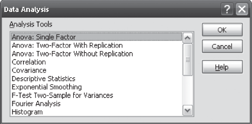
Figure 12.3 MS Excel Data Analysis dialog box
Microsoft Office 2007, copyright © 2007 Microsoft Corporation.
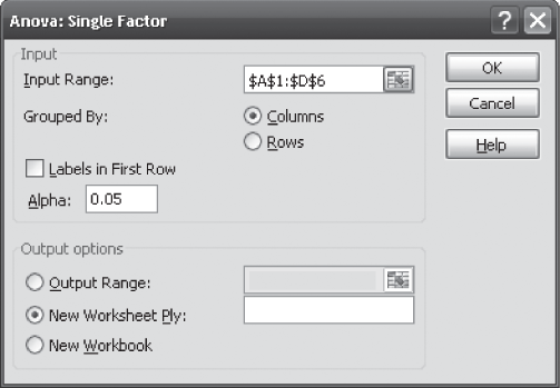
Figure 12.4 MS Excel Anova: Single Factor dialog box
Microsoft Office 2007, copyright © 2007 Microsoft Corporation.
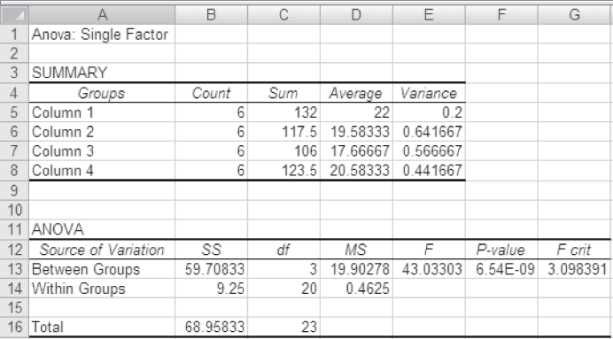
Figure 12.5 MS Excel output for Example 12.1
Microsoft Office 2007, copyright © 2007 Microsoft Corporation.
12.4.5 Using Minitab for Hypothesis Testing with the F Statistic for the Difference in the Means of More Than Two Populations
Minitab can also be used for hypothesis testing with F statistic for testing the difference in the means of more than two populations. As a first step, select Stat from the menu bar. A pull-down menu will appear on the screen, from this menu select ANOVA. Another pull-down menu will appear on the screen, from this pull-down menu select One-Way Unstacked. The One-Way Analysis of Variance dialog box will appear on the screen (Figure 12.6). By using Select, place samples in the Responses (in separate columns) box and place the desired Confidence level (Figure 12.6). Click OK, Minitab will calculate the F and p value for the test (shown in Figure 12.7).
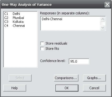
Figure 12.6 Minitab One-Way Analysis of Variance dialog box
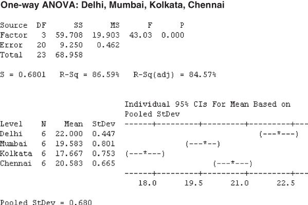
Figure 12.7 Minitab output for Example 12.1
12.4.6 Using SPSS for Hypothesis Testing with the F Statistic for the Difference in Means of More Than Two Populations
Hypothesis testing with F statistic for difference in means of more than two populations can be performed by SPSS. The process begins by selecting Analyse/Compare Means/One-Way ANOVA. The One-Way ANOVA dialog box will appear on the screen (Figure 12.8). Note that cities are coded using numbers. Delhi, Mumbai, Kolkata and Chennai are coded as 1, 2, 3, 4 respectively. Place Price in the Dependent List box and Coding (cities with coding) in the Factor box and click Options. The One-Way ANOVA: Options dialog box will appear on the screen. In this dialog box, from Statistics, click Descriptive and click Continue (Figure 12.9). The One-Way ANOVA dialog box will reappear on the screen. Click OK. The SPSS output as shown in Figure 12.10 will appear on the screen.
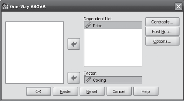
Figure 12.8 SPSS One-Way ANOVA dialog box
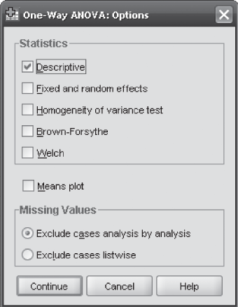
Figure 12.9 SPSS One-Way ANOVA: Options dialog box
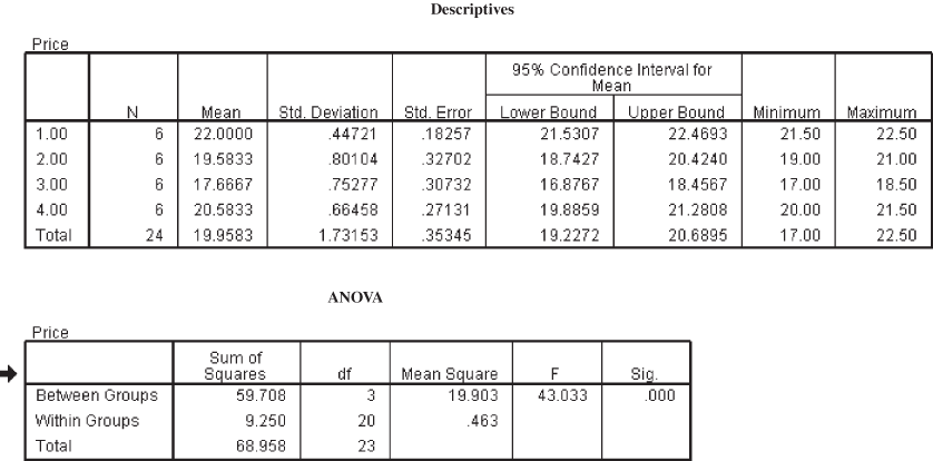
Figure 12.10 SPSS output for Example 12.1
Self-Practice Problems
12A1. Use the following data to perform one-way ANOVA

Use α = 0.05 to test the hypotheses for the difference in means.
12A2. Use the following data to perform one-way ANOVA
Use α = 0.01 to test the hypotheses for the difference in means.
12A3. A company is in the process of launching a new product. Before launching, the company wants to ascertain the status of its product as a second alternative. For doing so, the company prepared a questionnaire consisting of 20 questions on a five-point rating scale with 1 being “strongly disagree” and 5 being “strongly agree.” The company administered this questionnaire to 8 randomly selected respondents from five potential sales zones. The scores obtained from the respondents are given in the table. Use one-way ANOVA to analyse the significant difference in the scores. Take 90% as the confidence level.
12A4.

12.5 Randomized Block Design
We have already discussed that in one-way ANOVA the total variation is divided into two components: variations between the samples or columns, due to treatments and variation within the samples, due to error. There is a possibility that some of the variation, which was attributed to random error may not be due to random error, but may be due to some other measurable factors. If this measurable factor is included in the MSE, it will result in an increase in the MSE. Any increase in the MSE would result in a small F value (MSE being a denominator in the F-value formula), which would ultimately lead to the acceptance of the null hypothesis.
Like the completely randomized design, randomized block design also focuses on one independent variable of interest (treatment variable). Additionally, in randomized block design, we also include one more variable referred to as “blocking variable.” This blocking variable is used to control the confounding variable. Confounding variables, though not controlled by the researcher, can have an impact on the outcome of the treatment being studied. In Example 12.1, the selling price was different in the four metros. In this example, some other variable which is not controlled by the researcher may have an impact on the varying prices. This may be the tax policy of the state, transportation cost, etc. By including these variables in the experimental design, the possibility of controlling these variables can be explored. The blocking variable is a variable which a researcher wants to control but is not a treatment variable of interest. The term blocking has an agriculture origin where “blocking” refers to a block of land. For example, if we apply blocking in Example 12.1, under a given circumstance, each set of the four prices related to four metropolitan cities will constitute a block of sample data. Blocking refers to the division of experimental runs into smaller sub-groups or blocks.3 Blocking provides the opportunity for a researcher to compare prices one to one.
Like the completely randomized design, the randomized block design also focuses on one independent variable of interest (treatment variable). Additionally, in randomized block design, we also include one more variable referred to as “blocking variable.” This blocking variable is used to control the confounding variable. Confounding variables though not controlled by the researcher can have an impact on the outcome of the treatment being studied.
In case of a randomized block design, variation within the samples can be partitioned into two parts as shown in Figure 12.11.

Figure 12.11 Partitioning the SSE in randomized block design
Blocking variable is a variable which a researcher wants to control but is not a treatment variable of interest.
So, in randomized block design, the total sum of squares consists of three parts:
SST (total sum of squares) = SSC (sum of squares between columns) + SSR (sum of squares between rows) + SSE (sum of squares of errors)
12.5.1 Null and Alternative Hypotheses in a Randomized Block Design
It has already been discussed that in a randomized block design the total sum of squares consists of three parts. In light of this, the null and alternative hypotheses for the treatment effect can be stated as below:
Suppose if c samples are being analysed by a researcher then null hypothesis can be stated as:
![]()
The alternative hypothesis can be set as below:
H1: All treatment means are not equal
For blocking effect, the null and alternative hypotheses can be stated as below (when r rows are being analysed by a researcher):
![]()
The alternative hypothesis can be set as below:
H1: All blocking means are not equal
Formulas for calculating SST (total sum of squares) and mean squares in a randomized block design
SSC (sum of squares between columns) = ![]()
where c is the number of treatment levels (columns), r the number of observations in each treatment level (number of blocks), ![]() the sample mean of Group j (Column means), and
the sample mean of Group j (Column means), and ![]() the grand mean
the grand mean
and MSC(mean square) = ![]()
where SSC is the sum of squares between columns and c – 1 the degrees of freedom (number of columns – 1).
SSR (sum of squares between rows) = ![]()
where c is the number of treatment levels (columns), r the number of observations in each treatment level (number of blocks), ![]() the sample mean of Group i (row means), and
the sample mean of Group i (row means), and ![]() the grand mean
the grand mean
and MSR(mean square) = ![]()
where SSE is the sum of squares within columns, and r – 1 the degrees of freedom (number of rows – 1).
SSE (sum of squares of errors) = ![]()
where c is the number of treatment levels (columns), r the number of observations in each treatment level (number of blocks), ![]() the sample mean of Group i (row means), xj the sample mean of Group j (column means), xij the ith observation in Group j, and
the sample mean of Group i (row means), xj the sample mean of Group j (column means), xij the ith observation in Group j, and ![]() the grand mean
the grand mean
and MSE (mean square) = ![]()
where SSE is the sum of squares of errors and n – r – c + 1 = (c – 1)(r – 1) = degrees of freedom (number of observations – number of rows – number of columns + 1). Here, rc = n = number of observations.
12.5.2 Applying the F-Test Statistic
As discussed, the total sum of squares consists of three parts: SST(total sum of squares) = SSC (sum of squares between columns) + SSR (sum of squares between rows) + SSE (sum of squares of errors)
In case of two-way ANOVA, F value can be obtained as below:
F-test statistic in randomized block design
![]()
where MSC is the mean square column and MSE the mean square error.
with c – 1, degrees of freedom for numerator
n – r – c + 1 = (c – 1)(r – 1), degrees of freedom for denominator
and ![]()
where MSR is the mean square row and MSE the mean square error.
with r – 1 = degrees of freedom for numerator and
n – r – c + 1 = (c – 1)(r – 1), degrees of freedom for denominator.
For a given level of significance α, rules for acceptance or rejection of null hypothesis are as below:
For a given level of significance α, rules for acceptance or rejection of null hypothesis
Reject H0 if , Fcalculated > Fcritical . Otherwise, do not reject H0.
12.5.3 ANOVA Summary Table for Two-Way Classification
The results of ANOVA are usually presented in an ANOVA table (shown in Table 12.8). The entries in the table consist of SSC(sum of squares between columns), SSR (sum of squares between rows), SSE (sum of squares of errors), SST (total sum of squares); corresponding degrees of freedom (c – 1); (r – 1); (c – 1)(r – 1), and (n – 1); MSC (mean square column); MSR (mean square row) and MSE (mean square error); F values in terms of Ftreatment and Fblock. As discussed, in randomized block design when using software programs such as MS Excel, Minitab, and SPSS, summary table also includes p value. The p value allows a researcher to make inferences directly without taking help from the critical values of the F distribution.
Table 12.8 ANOVA Summary table for two-way classification

Example 12.2
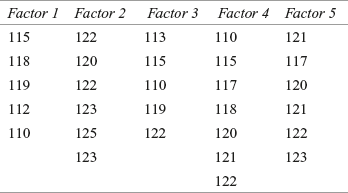
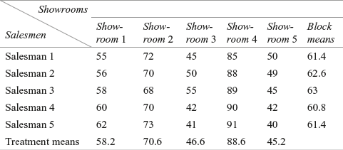
A company which produces stationary items wants to diversify into the photocopy paper manufacturing business. The company has decided to first test market the product in three areas termed as the north area, central area, and the south area. The company takes a random sample of five salesmen S1, S2, S3, S4, and S5 for this purpose. The sales volume generated by these five salesmen (in thousand rupees) and total sales in different regions is given in Table 12.9:
TABLE 12.9 Sales volume generated by five salesmen (in thousand rupees) and total sales in different regions (in thousand rupees)

Use a randomized block design analysis to examine:
- 1. Whether the salesmen significantly differ in performance?
- 2. Whether there is a significant difference in terms of sales capacity between the regions?
Take 95% as confidence level for testing the hypotheses.
Solution The seven steps of hypothesis testing can be performed as below:
Step 1: Set null and alternative hypotheses
The null and alternative hypotheses can be divided into two parts: For treatments (columns) and for blocks (rows).
For treatments (columns), null and alternative hypotheses can be stated as below:
![]()
and H1: All the treatment means are not equal
For blocks (rows), null and alternative hypotheses can be stated as below:
![]()
and H1: All the block means are not equal
Step 2: Determine the appropriate statistical test
F-test statistic in randomized block design
![]()
where MSC is the mean square column and MSE the mean square error.
with c – 1, degrees of freedom for numerator
n – r – c + 1 = (c – 1)(r – 1), degrees of freedom for denominator
and ![]()
where MSR is the mean square row and MSE the mean square error.
with r – 1, degrees of freedom for numerator
n – r – c + 1 = (c – 1)(r – 1), degrees of freedom for denominator.
Step 3: Set the level of significance
Let α = 0.05.
Step 4: Set the decision rule
For a given level of significance 0.05, the rules for acceptance or rejection of null hypothesis are as follows
Reject H0, if Fcalculated > Fcritical, otherwise do not reject H0.
For treatments, degrees of freedom = (c – 1) = (5 – 1) = 4
For blocks, degrees of freedom = (r – 1) = (3 –1) = 2
For error, degrees of freedom = (c – 1)(r – 1) = 4 × 2 = 8
Step 5: Collect the sample data
Sample data is given in Example 12.2. The treatment means and block means are shown in Table 12.10 as follows:
TABLE 12.10 Treatment means and block means for sales data

Step 6: Analyse the data
SSC (sum of squares between columns) = ![]()

= 183.066
SSR (sum of squares between rows) = ![]()
![]()
= 5.2
SSE (sum of squares of errors) = ![]()
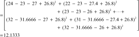
SST (total sum of squares of errors) = ![]()

= 200.40
![]()
![]()
![]()
![]()
![]()
The ANOVA summary table for Example 12.2 is shown in Table 12.11.
TABLE 12.11 ANOVA Summary table for Example 12.2

Step 7: Arrive at a statistical conclusion and business implication
At 95% confidence level, critical value obtained from the F table is F0.05, 4, 8 = 3.84 and F0.05, 2, 8 = 4.46.
The calculated value of F for columns is 30.17. This is greater than the tabular value (3.84) and falls in the rejection region. Hence, the null hypothesis is rejected and alternative hypothesis is accepted.
The calculated value of F for rows is 1.71. This is less than the tabular value (4.46) and falls in the acceptance region. Hence, the null hypothesis is accepted and alternative hypothesis is rejected.
There is enough evidence to believe that there is a significant difference in the performance of five salesmen in terms of generation of sales. On the other hand, there is no significant difference in the capacity of generating sales for the three regions. The result that indicates a difference in the sales volume generation capacity of the three regions may be due to chance. Therefore, the management should concentrate on individual salesmen rather than concentrating on regions.
12.5.4 Using MS Excel for Hypothesis Testing with the F Statistic in a Randomized Block Design
MS Excel can be used for hypothesis testing with F statistic in randomized block design. First select Tool from the menu bar. From this menu, select Data Analysis. The Data Analysis dialog box will appear on the screen. From this Data Analysis dialog box, select Anova: Two-Factor Without Replication and click OK (Figure 12.12). The Anova: Two-Factor Without Replication dialog box will appear on the screen. Enter the location of the sample in Input Range. Place the value of α and click OK (Figure 12.13). The MS Excel output as shown in (Figure 12.14) will appear on the screen.

Figure 12.12 MS Excel Data Analysis dialog box
Microsoft Office 2007, copyright © 2007 Microsoft Corporation.

Figure 12.13 MS Excel Anova: Two-Factor Without Replication dialog box
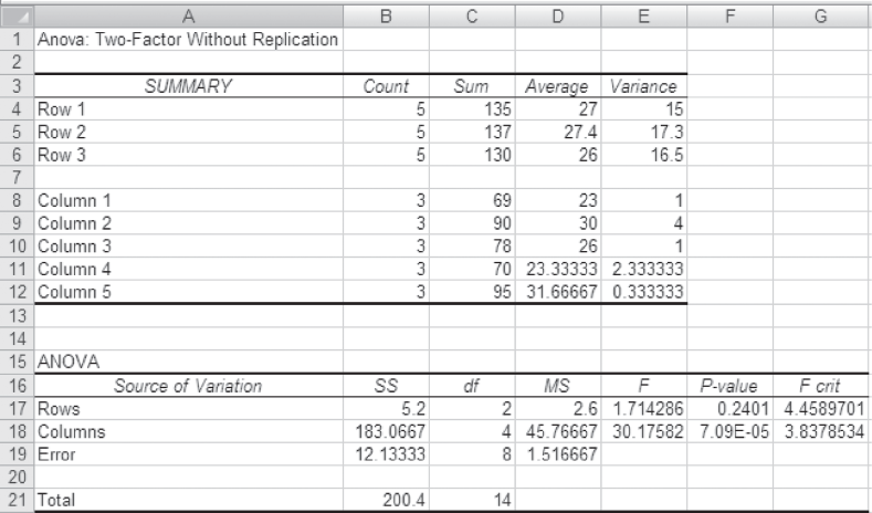
Figure 12.14 MS Excel output for Example 12.2
Microsoft Office 2007, copyright © 2007 Microsoft Corporation.
12.5.5 Using Minitab for Hypothesis Testing with the F Statistic in a Randomized Block Design
Minitab can be used for hypothesis testing with F statistic in randomized block design. The first step is to select Stat from the menu bar. A pull-down menu will appear on the screen, from this menu, select ANOVA. Another pull-down menu will appear on the screen, from this pull down menu, select Two-Way.
The Two-Way Analysis of Variance dialog box will appear on the screen (Figure 12.16). By using Select, place Sales volume generation in Response, region in the Row factor, and different salesmen in the Column factor. Place the desired confidence level in the appropriate box (Figure 12.16). Click OK, Minitab will calculate the F and p value for the test (shown in Figure 12.17).

Figure 12.16 Minitab Two-Way Analysis of Variance dialog box
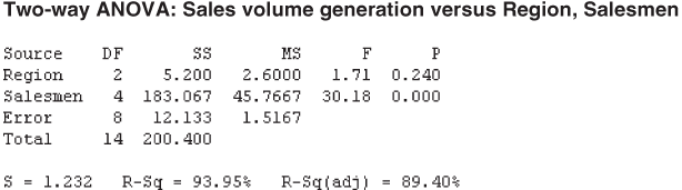
Figure 12.17 Minitab output for Example 12.2
When using Minitab for randomized block design, data should be arranged in a different manner (as shown in Figure 12.15). The observations should be “stacked” in one column. A second column should be created for row (block) identifiers and a third column should be created for column (treatment) identifiers (Figure 12.15).

Figure 12.15 Arrangement of data in Minitab sheet for randomized block design
SELF-PRACTICE PROBLEMS
12B1. The table below shows data in the form of a randomized block design.

Use a randomized block design analysis to examine:
- (1) Significant difference in the treatment level.
- (2) Significant difference in the block level.
Take 95% as confidence level for testing the hypotheses.
12B2. The table below shows data in form of a randomized block design

Use a randomized block design analysis to examine:
- (1) Significant difference in the treatment level.
- (2) Significant difference in the block level.
Take 90% as the confidence level for testing the hypotheses.
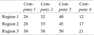
12B3. A researcher has obtained randomly selected sales data (in thousand rupees) of four companies: Company 1, Company 2, Company 3, and Company 4. These data are arranged in a randomized block design with respect to company and region. Use a randomized block design analysis to examine:
- (1) Significant difference in average sales of four different companies.
- (2) Significant difference in average sales of three different regions.
Take α = 0.05 for testing the hypotheses.
12.6 Factorial Design (Two-way ANOVA)
In some real-life situations, a researcher has to explore two or more treatments simultaneously. This type of experimental design is referred to as factorial design.
In some real-life situations, a researcher has to explore two or more treatments simultaneously. This type of experimental design is referred to as factorial design. In a factorial design, two or more treatment variables are studied simultaneously. For example, in the previous example, we had discussed the variation in performance of salesmen due to one blocking variable, region. Salesmen performance may also depend upon various other variables such as support provided by the company, attitude of a particular salesman, support from the dealer network, support from the retailer, etc. All these four variables (and many other variables depending upon the situation) can be included in the experimental design and can be studied simultaneously. In this section, we will study the factorial design with two treatment variables.
Factorial design provides an opportunity to study the interaction effect of two treatment variables.
Factorial design has many advantages over completely randomized design. If we use completely randomized design for measuring the effect of two treatment variables, we will have to apply two complete randomized designs. Factorial design provides a platform to analyse both the treatment variables simultaneously in one experimental design. In a factorial design, a researcher can control the effect of multiple treatment variables. In addition, factorial design provides an opportunity to study the interaction effect of two treatment variables. It is important to understand that the randomized block design concentrates on one treatment (column) and control for a blocking effect (row effect). Randomized block design does not provide the opportunity to study the interaction effect of treatment and block. This facility is available only in factorial design.
12.6.1 Null and Alternative Hypotheses in a Factorial Design
A two-way analysis of variance is used to test the hypothesis of a factorial design having two factors. In light of this, the null and alternative hypotheses for the treatment effect can be stated as below:
Row effect: H0: All the row means are equal.
H1: All the row means are not equal.
Column effect: H0: All the column means are equal.
H1: All the column means are not equal.
Interaction effect: H0: Interaction effects are zero.
H1: Interaction effect is not zero (present).
12.6.2 Formulas for Calculating SST (Total Sum of Squares) and Mean Squares in a Factorial Design (Two-Way Analysis of Variance)
SSC (sum of squares between columns) = ![]()
where c is the number of column treatments, r the number of row treatments, n the number of observations in each cell, ![]() the sample mean of Group j, and
the sample mean of Group j, and ![]() the grand mean
the grand mean
and MSC (mean square) = ![]()
where SSC is the sum of squares between columns and c – 1 the degrees of freedom (number of columns – 1).
SSR (sum of squares between rows) = ![]()
where c is the number of column treatments, r the number of row treatments, n the number of observations in each cell, ![]() the sample mean of Group i (row means), and
the sample mean of Group i (row means), and ![]() the grand mean
the grand mean
and MSR (mean square) = ![]()
where SSR is the sum of squares between rows and r – 1 the degrees of freedom (number of rows – 1).
SSI (sum of squares interaction) = ![]()
where c is the number of column treatments, r the number of row treatments, n the number of observations in each cell, ![]() the sample mean of Group i (row means),
the sample mean of Group i (row means), ![]() the sample mean of Group j (column means),
the sample mean of Group j (column means), ![]() the mean of the cell corresponding to ith row and jth column (cell mean), and
the mean of the cell corresponding to ith row and jth column (cell mean), and ![]() the grand mean
the grand mean
and MSI (mean square) = ![]()
where SSI is the sum of squares interaction and (r – 1)(c – 1) the degrees of freedom.
SSE (sum of squares errors) = ![]()
where c is the number of column treatments, r the number of row treatments, n the number of observations in each cell, xijk the individual observation, ![]() the mean of the cell corresponding to ith row and jth column (cell mean)
the mean of the cell corresponding to ith row and jth column (cell mean)
and MSE (mean square) = ![]()
where SSE is the sum of squares of errors and rc (n – 1) the degrees of freedom.
SST (total sum of squares) = ![]()
where c is the number of column treatments, r the number of row treatments, n the number of observations in each cell, xijk the individual observation, ![]() the grand mean.
the grand mean.
and MST (mean square) = ![]()
where SST is the total sum of squares and N – 1 the degrees of freedom (total number of observa- tions – 1).
12.6.3 Applying the F-Test Statistic
As discussed, the total sum of squares consists of four parts: SST (total sum of squares) = SSC (sum of squares between columns) + SSR (sum of squares between rows) + SSI (sum of squares interaction) + SSE (sum of squares of errors)
In case of two-wayANOVA, the F value can be obtained as below:
F-test statistic in two-way ANOVA
![]()
where MSC is the mean square column and MSE the mean square error
with c – 1, degrees of freedom for numerator and
rc (n – 1) degrees of freedom for denominator.
![]()
where MSR is the mean square row and MSE the mean square error
with r – 1, degrees of freedom for numerator and
rc (n – 1) degrees of freedom for denominator.
![]()
where MSI is the mean square interaction and MSE the mean square error
with (r – 1)(c – 1), degrees of freedom for numerator and
rc (n – 1), degrees of freedom for denominator.
For a given level of significance α, rules for acceptance or rejection of null hypothesis are as below:
For a given level of significance α, rules for acceptance or rejection of null hypothesis
Reject H0, if Fcalculated > Fcritical, otherwise, do not reject H0.
12.6.4 ANOVA Summary Table for Two-Way ANOVA
The result of ANOVA for a factorial design is usually presented in an ANOVA table (shown in Table 12.12).The entries in the table consist of SSC (sum of squares between columns), SSR (sum of squares between rows), SSI (sum of squares interaction), SSE (sum of squares of errors), SST (total sum of squares); corresponding degrees of freedom (c – 1); (r – 1); (c – 1)(r – 1); rc (n – 1) and (N – 1); MSC (mean square column); MSR (mean square row); MSI (mean square interaction) and MSE (mean square error); F values in terms of Ftreatment; Fblock , and Finteraction. Software programs such as MS Excel, Minitab, and SPSS, calculate p-value test in the ANOVA table, which allows a researcher to make inferences directly without taking help from the critical values of the F distribution.
Table 12.12 ANOVA Summary table for two-way ANOVA

Example 12.3
Chhattisgarh Steel and Iron Mills is a leading steel rod manufacturing company of Chhattisgarh. The company produces 8-metre long steel rods, which are used in the construction of buildings. The company has four machines which manufacture steel rods in three shifts. The company’s quality control officer wants to test whether there is any difference in the average length of the iron rods by shifts or by machines. Data given in Table 12.13 is organized by machines and shifts obtained through a random sampling process. Employ a two-way analysis of variance and determine whether there are any significant differences in effects. Take α = 0.05.
TABLE 12.13 Length of the iron rod in different shifts and produced by different machines

Solution The seven steps of hypothesis testing can be performed as below:
Step 1: Set null and alternative hypotheses
The null and alternative hypotheses can be stated as below:
Row effect: H0: All the row means are equal.
H1: All the row means are not equal.
Column effect: H0: All the column means are equal.
H1: All the column means are not equal.
Interaction effect: H0: Interaction effects are zero.
H1: Interaction effect is not zero (present).
Step 2: Determine the appropriate statistical test
F-test statistic in two-way ANOVA
![]()
where MSC is the mean square column and MSE the mean square error
with c – 1, degrees of freedom for numerator and
rc (n – 1) degrees of freedom for denominator.
![]()
where MSR is the mean square row and MSE the mean square error
with r – 1, degrees of freedom for numerator and
rc (n – 1) degrees of freedom for denominator.
![]()
where MSI is the mean square interaction and MSE is the mean square error. with (r – 1)(c – 1), degrees of freedom for numerator and
rc (n – 1) degrees of freedom for denominator.
Step 3: Set the level of significance
Let α = 0.05.
Step 4: Set the decision rule
For a given level of significance α, the rules for acceptance or rejection of the null hypothesis are
Reject H0 if Fcalculated > Fcritical, otherwise, do not reject H0.
For treatments, degrees of freedom = (c – 1) = (3 – 1) = 2
For blocks, degrees of freedom = (r – 1) = (4 – 1) = 3
For interaction, degrees of freedom = (c – 1)(r – 1) = 2 × 3 = 6
For error, degrees of freedom rc(n – 1) = 4 × 3 × 2 = 24
Step 5: Collect the sample data
The sample data is given in Table 12.14:
Table 12.14 Sample data for Example 12.3 and computation of different means

![]() Grand mean = 7.99055
Grand mean = 7.99055
Step 6: Analyse the data
SSR (sum of squares between rows) = ![]()

= 1.02077
SSC (sum of squares between columns) = ![]()

= 0.00376
SSI (sum of squares interaction) = ![]()

= 0.02527
SSE (sum of squares errors) = ![]()

= 0.0568
SST (total sum of squares) = ![]()

= 1.106589
MSR (mean square)![]()
MSC (mean square)![]()
MSI (mean square) ![]()
MSE (mean square)![]()
![]()
![]()
![]()
TABLE 12.15 ANOVA Summary table for Example 12.3

Table 12.15 presents the ANOVA summary table for Example 12.3.
Step 7: Arrive at a statistical conclusion and business implication
At 95% confidence level, the critical value obtained from the table is F0.05, 2, 24 = 3.40, F0.05, 3, 24 = 3.01 and F0.05, 6, 24 = 2.51.
The calculated value of F for columns is 0.79. This is less than the tabular value (3.40) and falls in the acceptance region. Hence, the null hypothesis is accepted and the alternative hypothesis is rejected.
The calculated value of F for rows is 143.77. This is greater than the tabular value (3.01) and falls in the rejection region. Hence, the null hypothesis is rejected and alternative hypothesis is accepted.
The calculated value of F for interaction is 1.78. This is less than the tabular value (2.51) and falls in the acceptance region. Hence, the null hypothesis is accepted and the alternative hypothesis is rejected.
The result indicates that there is a significant difference in the steel rods produced by different machines. The results also indicate that the difference in the length of the steel rods produced in three shifts are not significant and the differences obtained (as exhibited from the sample result) are due to chance. Additionally, interaction between machines and shifts is also not significant and differences (as exhibited from the sample result) are due to chance. Therefore, the management must focus on the machines to ensure that the steel rods produced by all the machines are uniform.
12.6.5 Using MS Excel for Hypothesis Testing with the F Statistic in a Factorial Design
First, select Tool from the menu bar. From this menu, select Data Analysis. The Data Analysis dialog box will appear on the screen. From the Data Analysis dialog box, select Anova: Two-Factor With Replication and click OK (Figure 12.18). The Anova: Two-Factor With Replication dialog box will appear on the screen. Enter the location of the sample in Input Range. Place the value of Rows per sample (number of observations per cell). Place the value of α and click OK (Figure 12.19). The MS Excel output as shown in (Figure 12.20) will appear on the screen. The arrangement of data in MS Excel worksheet for a factorial design (two-way ANOVA) is shown in Figure 12.21.
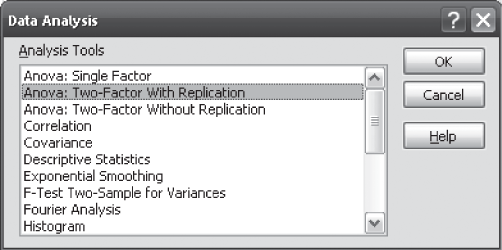
Figure 12.18 MS Excel Data Analysis dialog box
Microsoft Office 2007, copyright © 2007 Microsoft Corporation.

Figure 12.19 MS Excel Anova: Two-Factor With Replication dialog box
Microsoft Office 2007, copyright © 2007 Microsoft Corporation.
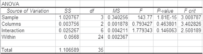
Figure 12.20 MS Excel output for Example 12.3
Microsoft Office 2007, copyright © 2007 Microsoft Corporation.

Figure 12.21 Arrangement of data in MS Excel worksheet for a factorial design (Example 12.3)
Microsoft Office 2007, copyright © 2007 Microsoft Corporation.
12.6.6 Using Minitab for Hypothesis Testing with the F Statistic in a Randomized Block Design
Select Stat from the menu bar. A pull-down menu will appear on the screen, from this menu, select ANOVA. Another pull-down menu will appear on the screen, from this pull-down menu, select Two-Way Analysis of Variance.
The Two-Way Analysis of Variance dialog box will appear on the screen (Figure 12.22). By using Select, place Mean Length in the Response box, Machine in the Row factor box, and Shift in the Column factor box. Check Display means against Row factor and Column factor. Place the desired confidence level in the Confidence level box (Figure 12.22). Click OK, Minitab will calculate the F and p value for the test (shown in Figure 12.23). The placement of data in the Minitab worksheet should be done in the same manner as described for Example 12.2 in the procedure of using Minitab for hypothesis testing with F statistic in a randomized block design.

Figure 12.22 Minitab Two-Way Analysis of Variance dialog box

Figure 12.23 Minitab output for Example 12.3
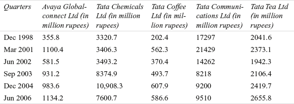
Example 12.4
Suppose a researcher wants to know the difference in average income (in million rupees) of five different companies of the Tata Group. These companies are: Avaya Globalconnect Ltd (Tata Telecom Ltd), Tata Chemicals Ltd, Tata Coffee Ltd, Tata Communications Ltd, and Tata Tea Ltd. With access to the quarterly sales data of these companies, the researcher has randomly selected the income of these companies for six quarters (Table 12.16)
Table 12.16 Income of five companies of the Tata Group in six randomly selected quarters

Source: Prowess (V. 3.1), Centre for Monitoring Indian Economy Pvt. Ltd, Mumbai, accessed November 2008, reproduced with permission.
Use one-way ANOVA to analyse the significant difference in the average quarterly income of companies. Take 95% as the confidence level.
Solution The seven steps of hypotheses testing can be performed as below:
Step 1: Set null and alternative hypotheses
The null and alternative hypotheses can be stated as below:
H0: μ1= μ2 = μ4 = μ5
and H1: All the means are not equal
Step 2: Determine appropriate statistical test
The appropriate test statistic is F-test statistic in one-way ANOVA
![]()
where MSC is the mean square column and MSE the mean square error.
Step 3: Set the level of significance
Alpha has been specified as 0.05. So, confidence level is 95%.
Step 4: Set the decision rule
For a given confidence level 95%, rules for acceptance or rejection of null hypothesis
Reject H0, if F(Calculated) > FU (Upper-tail value of F),
otherwise, do not reject H0.
In this example, for the numerator and denominator, the degree of freedom is 4 and 25, respectively. The critical F value is F0.05, 4, 25 = 2.76.
Step 5: Collect the sample data
The sample data is shown in Table 12.19:
Solution The seven steps of hypothesis testing can be performed as below:
Step 1: Set null and alternative hypotheses
The null and alternative hypotheses can be divided in two parts: For columns (showrooms) and for rows (salesmen).
For columns (showrooms), null and alternative hypotheses can be stated as below:
![]()
and H1: All the column means are not equal
For rows (salesmen), null and alternative hypotheses can be stated as below:
![]()
and H1: All the row means are not equal
Step 2: Determine the appropriate statistical test
F-test statistic in randomized block design
![]()
where MSC is the mean square column and MSE the mean square error.
with c – 1, degrees of freedom for numerator and
n – r – c + 1 = (c – 1)(r – 1), degrees of freedom for denominator.
![]()
where MSR is the mean square row and MSE the mean square error
with r – 1, degrees of freedom for numerator and
n – r – c + 1 = (c – 1)(r – 1), degrees of freedom for denominator.
Step 3: Set the level of significance
Level of significance α is taken as 0.01.
Step 4: Set the decision rule
For a given level of significance 0.01, rules for acceptance or rejection of null hypothesis
Reject H0, if Fcalculated > Fcritical, otherwise do not reject H0.
Step 5: Collect the sample data
The sample data is given in Table 12.23.
Table 12.23 Column means and row means for Example 12.6
Step 6: Analyse the data
Figure 12.37 exhibits the MS Excel output for Example 12.6. It shows the column descriptive statistics, row descriptive statistics, and the ANOVA table.
Step 7: Arrive at a statistical conclusion and business implication
At 1% level of significance, the critical value obtained from the table is F0.01, 4, 16 = 4.77.
The calculated value of F for columns is 99.54. The calculated value of F (99.54) is greater than the critical value of F (4.77) and falls in the rejection region. Hence, null hypothesis is rejected and alternative hypothesis is accepted.
Calculated value of F for rows is 0.25. This is less than the tabular value (4.77) and falls in the acceptance region. Hence, null hypothesis is accepted and alternative hypothesis is rejected.
There is enough evidence to believe that there is a significant difference in the five showrooms in terms of the generation of sales volume. There is no significant difference in the sales volume generation capacity of the five salesmen. The result which we have obtained in terms of difference in sales volume generation capacity of the five salesmen may be due to chance. So, the management should concentrate on the different showrooms in order to generate equal sales from all the showrooms.
Solution The seven steps of hypothesis testing can be performed as follows:
Step 1: Set null and alternative hypotheses
The null and alternative hypotheses can be divided in two parts: For columns (products) and for rows (customers).
For columns (products), null and alternative hypotheses can be stated as below:
![]()
and H1: All the column means are not equal
For rows (customers), null and alternative hypotheses can be stated as below:
![]()
and H1: All the row means are not equal
Step 2: Determine the appropriate statistical test
F-test statistic in randomized block design
![]()
where MSC is the mean square column and MSE the mean square error.
with c – 1, degrees of freedom for numerator and
n – r – c + 1 = (c – 1)(r – 1), degrees of freedom for denominator.
and ![]()
where MSR is the mean square row and MSE the mean square error.
with r – 1, degrees of freedom for numerator and n – r – c + 1 = (c – 1)(r – 1), degrees of freedom for denominator.
Step 3: Set the level of significance
Level of significance α is taken as 0.05.
Step 4: Set the decision rule
For a given level of significance 0.05, rules for acceptance or rejection of null hypothesis:
Reject H0 if Fcalculated > Fcritical, otherwise, do not reject H0
Step 5: Collect the sample data
The sample data is given in Table 12.24.
Step 6: Analyse the data
Figure 12.38 exhibits the Minitab output and Figure 12.39 exhibits the partial MS Excel for Example 12.7.
Step 7: Arrive at a statistical conclusion and business implication
At 5% level of significance, the critical value obtained from the table is F0.05, 9, 36 = 2.15 and F0.05, 4, 36 = 2.63.
For columns, the calculated value of F is 35.29. Calculated value of F (35.29) is greater than the critical value of F (2.63) and falls in the rejection region. Hence, null hypothesis is rejected and alternative hypothesis is accepted.
For rows the calculated value of F is 0.65. This value is less than the tabular value (2.15) and falls in the acceptance region. Hence, null hypothesis is accepted and the alternative hypothesis is rejected.

Figure 12.38 Minitab output exhibiting ANOVA table and summary statistics for Example 12.7
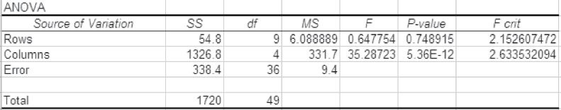
Figure 12.39 Partial MS Excel output exhibiting ANOVA table for Example 12.7
There is enough evidence to believe that there is a significant difference in terms of mean scores for five different products. There is no significant difference in terms of scores obtained by 10 different customers. The result that we have obtained may be due to chance. So, the management should concentrate on ensuring customers loyalty for different products.
Self-Practice Problems
12C1. Perform two-way ANOVA on the data arranged in the form of a two-way factorial design below:

12C2. Perform two-way ANOVA analysis on the data arranged in form of a two-way factorial design as below:

12C3. A company organized a training programme for three categories of officers: sales managers, zonal managers, and regional managers. The company also considered the education level of the employees. Based on their qualifications, officers were also divided into three categories: graduate, post graduates, and doctorates. The company wants to ascertain the effectiveness of the training programme on employees across designation and educational levels. The scores obtained from randomly selected employees across different categories are given below:


Employ a two-way analysis of variance and determine whether there are significant differences in effects. Take α = 0.05
12.7 Post hoc comparisons in ANOVA
In example 12.1, we have discussed null hypothesis and alternative hypothesis as:
![]()
and ![]() All the means are not equal
All the means are not equal
As the overall ANOVA results are significant, we accepted the above alternative hypothesis as “all the means are not equal.” Here, we are not very clear that all the means are different from one another or there is only one mean different from others. Post hoc (after-the-fact) compares two means at a time and tests following six pairs of hypotheses:
![]()
![]()
![]()
![]()
![]()
![]()
ANOVA is used initially to determine a significant effect of independent variable considered for the study. Once a significant effect is achieved, post hoc multiple comparison is then used to find out specific pairs or combinations of means that are not equal.4 Multiple comparisons are based on the concept of family wise type I error rate. This is based on the similar concept of type I error with little bit of logical modification. For example, consider testing three null hypotheses at 90% confidence level. The probability of making a correct decision is 0.90. The probability of making three consecutive correct decisions is![]() Hence, the probability of making at least one correct decision is
Hence, the probability of making at least one correct decision is ![]() This is referred to as family wise type I error.
This is referred to as family wise type I error.
This is obvious that with the increased number of post hoc comparison, family wise type I error rate also increases. For example, the probability of making at least one correct decision, for testing five null hypotheses is: ![]() Hence, the level of significance increases for a family of tests when compared with individual test. Many tests are available to check this family wise error rate. Three most common post hoc procedures are: Tukey, Scheffc and Bonferroni.5 In this section, we will focus on discussing Tuckey HSD test. Figure 12.24 exhibits post hoc comparisons for example 12.1. At 90% confidence level, all the pair wise alternative hypotheses are being accepted.
Hence, the level of significance increases for a family of tests when compared with individual test. Many tests are available to check this family wise error rate. Three most common post hoc procedures are: Tukey, Scheffc and Bonferroni.5 In this section, we will focus on discussing Tuckey HSD test. Figure 12.24 exhibits post hoc comparisons for example 12.1. At 90% confidence level, all the pair wise alternative hypotheses are being accepted.
12.7.1 Using SPSS for Post Hoc Comparision
For running post hoc comparisons in SPSS, select Analyze/General Linear Model/Univariate. Univariate dialogue box as exhibited in Figure 12.25 will appear on the screen. Place price in Dependent Variable box and cities in Fixed Factor(s) box and click Post Hoc.
Univariate: Post Hoc Multiple Comparisons for Observed Means dialogue box will appear on the screen. Place cities in Post Hoc tests for. From Equal Variances Assumed select Tukey and click Continue (see Figure 12.26). Univariate dialogue box will reappear on the screen and click OK. Partial output of SPSS as exhibited in Figure 12.24 will appear on the screen.

Figure 12.25 Dialogue Box for ‘SPSS Univariate’
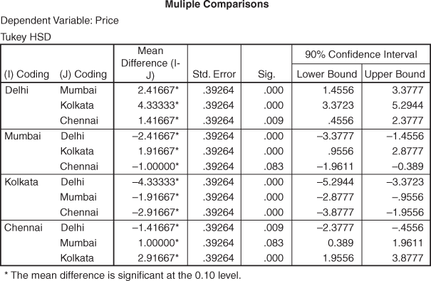
Figure 12.24 Post hoc comparisons for Example 12.1

Figure 12.26 Dialogue box for ‘SPSS Univariate: Post Hoc Multiple Comparisons for Observed Means’
12.8 Three-Way ANOVA
For understanding three-way ANOVA, we will modify Example 12.3. For making it three way, we have inserted one more factor, three levels of operator as operator A, operator B and operator C. For modification in the problem, three machines machine 1, machine 2 and machine 3 are being considered. For executing three-way ANOVA, three shifts are being considered. So, design becomes an example of ![]() ANOVA where there are three machines, three shifts and three operators. Table 12.16 presents this modified example. Three-way ANOVA will present three main effects, three two-factor interaction effect and one three-factor interaction effect. So, in a three-way ANOVA following seven hypotheses can be constructed and further tested:
ANOVA where there are three machines, three shifts and three operators. Table 12.16 presents this modified example. Three-way ANOVA will present three main effects, three two-factor interaction effect and one three-factor interaction effect. So, in a three-way ANOVA following seven hypotheses can be constructed and further tested:
Hypothesis 1: Main effect for machine is present.
Hypothesis 2: Main effect for shift is present.
Hypothesis 3: Main effect for operator is present.
Hypothesis 4: Significant interaction between machine and shift is present.
Hypothesis 5: Significant interaction between machine and operator is present.
Hypothesis 6: Significant interaction between shift and operator is present.
Hypothesis 7: Significant interaction between machine, shift and operator is present.
Table 12.16 Modified Example 12.3 for executing a three-way ANOVA


Figure 12.27 Main effect and interaction effect for modified example
Figure 12.27 is the main SPSS output for three-way ANOVA. At 90% confidence level, the main effect of machine, shift and operator are found to be significant. Interaction effect of machine* shift and machine* operator are not significant. Interaction effect of shift* operator is also significant. In addition, interaction effect of machine* shift* operator is also found to be significant. In this manner, hypothesis 1, hypothesis 2, hypothesis 3, hypothesis 6 and hypothesis 7 are accepted. Hypothesis 4 and hypothesis 5 are being rejected. Similarly, on the basis of p value, post hoc comparison presented in figures 12.28, 12.29 and 12.30 can be easily interpreted.
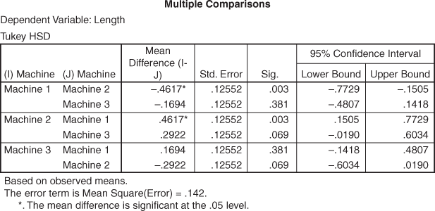
Figure 12.28 Multiple comparisons for machines
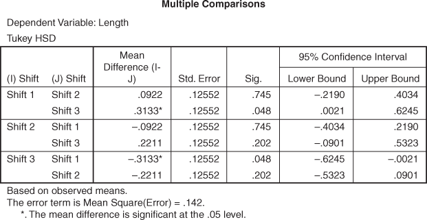
Figure 12.29 Multiple comparisons for shifts

Figure 12.30 Multiple comparisons for operators
12.9 Multivariate Analysis of Variance (MANOVA): A One-way Case
In this chapter, we have discussed the case of one-way ANOVA with one metric dependent variable and more than two levels of independent variable. In two-way ANOVA and three-way ANOVA, cases discussed have one dependent variable and two or multiple independent variables, respectively. In this progression of models, independent variables were changed but dependent variable remained a single metric variable throughout. A study to examine the impact of one or more independent variables on two or more dependent variables is referred to as multivariate analysis of variance (MANOVA). So, MANOVA includes two or multiple dependent variables. In the beginning of the chapter, we have discussed some assumptions of ANOVA. MANOVA has to qualify these assumptions as well. In addition, MANOVA is based on some supplementary assumptions listed below:
- Dependent variables must be multivariate, normally distributed within each group of independent variables. This assumption is referred to as multivariate normality.
- There should be homogeneity of variances – covariances matrices.
- Sample size must be adequately large.
- Absence of multi-colinearity for dependent variables.
It should be noted that violation of any assumption of ANOVA / MANOVA and its corrective action is beyond the scope of this chapter.
In this section, we will take a simple case of multivariate analysis of variance (one-way). For understanding the concept of multivariate analysis of variance (one-way), we will modify Problem 12.1 by inserting one more dependent variable. Table 12.17 exhibits four cities and two dependent variables – Brand 1 and Brand 2. With the insertion of two dependent variables, the one-way problem discussed as Problem 12.1 got converted into a multivariate analysis of variance (one-way) problem. SPSS output (partial) for modified example is given from Figure 12.31 to Figure 12.33.
Table 12.17 Price per pack of biscuits for two brands: Brand 1 and Brand 2
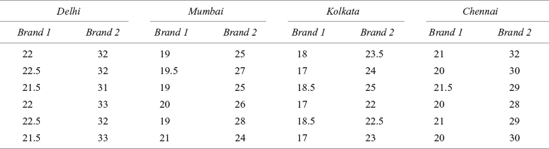

Figure 12.31 Descriptive statistics for MANOVA example
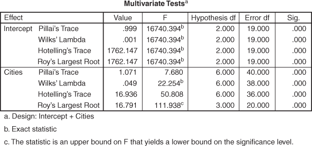
Figure 12.32 Multivariate Tests for MANOVA example
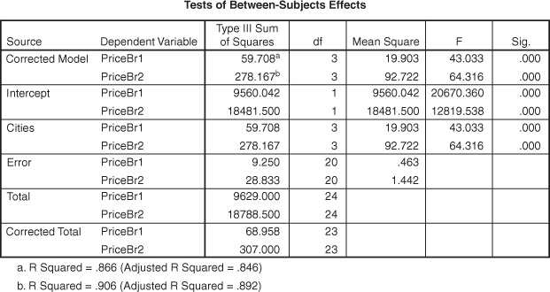
Figure 12.33 Tests of Between-Subjects Effects for MANOVA example
Figure 12.31 presents descriptive statistics (mean and standard deviation) for the MANOVA example. Figure 12.32 presents multivariate test for the MANOVA example and indicates four statistics: Pillai’s Trace, Wilks’ Lambda, Hotelling’s Trace and Roy’s largest root. Each statistics is being used for testing the null hypothesis that the population means for the multiple dependent variables are equal across the group. Each statistic is indicating different F values, so, right selection of any of these statistics is extremely important.
Hotelling’s Trace is used when independent variable has exactly two groups. In case, independent variables have more than two groups, Wilks’ Lambda should be used. It is similar to F-test of univariate ANOVA. Free from restriction of independent variables group, Pillai’s Trace and Roy’s largest root can be used for any number of independent variables categories. Pillai’s Trace seems to be widely applied powerful statistic but its power is being compromised when sample size in the independent sample group is unequal. Violation of homogeneity of variance assumption of MANOVA also restricts use of this statistic. Roy’s largest root is similar to Pillai’s Trace but not advisable with platykurtic distribution. From the last column of the Figure 12.32, we can see a significant p value pertaining to all the statistics. This is the indication of acceptance of alternative hypothesis that population means for the multiple dependent variables are not equal across the group. For our example, Wilks’ Lambda can be considered as an appropriate statistic for testing the equal mean hypotheses across the group.
12.9.1 Using SPSS for MANOVA
For running MANOVA in SPSS, select Analyze/General Linear Model/Multivariate. As exhibited in Figure 12.34, the Multivariate dialogue box will appear on the screen. Place price for Brand 1 and Brand 2 in Dependent Variables box and cities in Fixed Factor(s) box; and repeat the procedure as discussed for post hoc comparisons.

Figure 12.34 SPSS Multivariate dialogue box
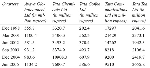
Example 12.4
Suppose a researcher wants to know the difference in average income (in million rupees) of five different companies of the Tata Group. These companies are: Avaya Globalconnect Ltd (Tata Telecom Ltd), Tata Chemicals Ltd, Tata Coffee Ltd, Tata Communications Ltd, and Tata Tea Ltd. With access to the quarterly sales data of these companies, the researcher has randomly selected the income of these companies for six quarters (Table 12.18)
Table 12.18 Income of five companies of the Tata Group in six randomly selected quarters
Source: Prowess (V. 3.1), Centre for Monitoring Indian Economy Pvt. Ltd, Mumbai, accessed November 2008, reproduced with permission.
Use one-way ANOVA to analyse the significant difference in the average quarterly income of companies. Take 95% as the confidence level.
TABLE 12.19 Sample data for Tata Group Example 12.4
Step 6: Analyse the data
The MS Excel analysis of the data is shown in Figure 12.35.
Step 7: Arrive at a statistical conclusion and business implication
At 95% confidence level, the critical value obtained from the table is F0.05,4,25 = 2.76. The calculated value of F is 22.34, which is greater than the tabular value (critical value) and falls in the rejection. Hence, the null hypothesis is rejected and the alternative hypothesis is accepted.
Therefore, there is a significant difference in the average quarterly income of companies.
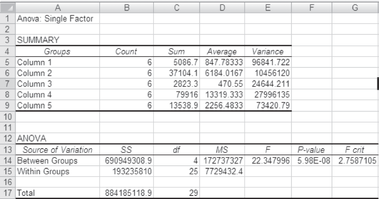
Figure 12.35 MS Excel output exhibiting summary statistics and ANOVA table for Example 12.4
Example 12.5
A researcher wants to estimate the average quarterly difference in the net sales of five companies of JK group. Due to some reasons, he could not obtain the data on average net sales of these companies. He has taken net sales of the five companies for six randomly selected quarters as indicated in Table 12.20.
Table 12.20 Net sales of five companies of JK group in different randomly selected quarters
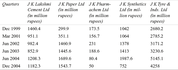
Source: Prowess (V. 3.1), Centre for Monitoring Indian Economy Pvt. Ltd, Mumbai, accessed November 2008, reproduced with permission.
Use one-way ANOVA to analyse the significant difference in the average quarterly net sales. Take 90% as the confidence level.
Solution The seven steps of hypothesis testing can be performed as below:
Step 1: Set null and alternative hypotheses
The null and alternative hypotheses can be stated as below:
![]() = μ5
= μ5
and H1: All the means are not equal
Step 2: Determine the appropriate statistical test
The appropriate test statistic is F-test statistic in one-way ANOVA
![]()
where MSC is the mean square column and MSE is the mean square error.
Step 3: Set the level of significance
For testing the hypotheses, alpha has been specified as 0.05 (α = 0.05).
Step 4: Set the decision rule
For a given level of significance (α = 0.05), rules for acceptance or rejection of the null hypothesis
Reject H0, if F(Calculated) > FU (Upper-tail value of F),
otherwise, do not reject H0.
The degree of freedom for numerator and denominator is 4 and 25, respectively. The critical F value is F0.10, 4, 25 = 2.18.
Step 5: Collect the sample data
The sample data is given in Table 12.21:
Table 12.21 Sample data for Example 12.5
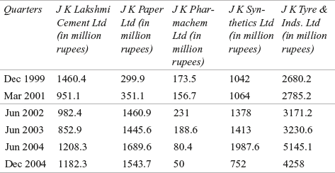
Step 6: Analyse the data
The MS Excel analysis of the data is shown in Figure 12.36.
Step 7: Arrive at a statistical conclusion and business implication
The critical value obtained from the table is F0.10, 4, 25 = 2.18. The computed value of F is obtained as 30.47. This computed value (30.47) is greater than the critical value (2.18) and falls in the rejection region. Hence, null hypothesis is rejected and alternative hypothesis is accepted.
At 90% confidence level, there is a significant difference between the net sales of five companies of the JK group. The researcher is now 90% confident that there exists a significant difference between the net sales of five companies of JK group.
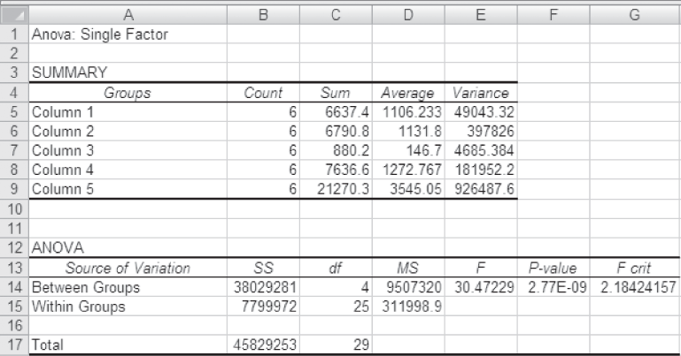
Figure 12.36 Excel output exhibiting summary statistics and ANOVA table for Example 12.5
Microsoft Office 2007, copyright © 2007 Microsoft Corporation.
Example 12.6
A leading shoe manufacturer has 500 showrooms across the country. The company wants to know the average difference in sales of these showrooms. It also wants to know the average sales difference between salesmen. For ascertaining the productivity of different salesmen, the company has adopted a practice of retaining one salesman for three months at one showroom. The company randomly selected five showrooms and five salesmen from each of the showrooms. Table 12.22 exhibits the average sales (in thousand rupees) from showrooms and the individual contribution of the five salesmen placed at different showrooms.
Table 12.22 Sales volume generated by five salesmen and sales from different showrooms (in thousand rupees)

Use a randomized block design analysis to examine
(1) Whether the salesmen significantly differ in productivity?
(2) Whether there is a significant difference between the average sales of showrooms?
Take 99% as confidence level for testing the hypotheses.

Figure 12.37 MS Excel output exhibiting summary statistics and ANOVA table for Example 12.6
Microsoft Office 2007, copyright © 2007 Microsoft Corporation.
Example 12.7
The vice president of a firm that enjoys market monopoly is concerned about the entry of a multinational firm in the market. He wants to analyse the brand loyalty for the firm’s products. The firm has randomly selected 10 customers and obtained their scores on a brand-loyalty measuring questionnaire. This questionnaire consisted of 10 questions with each question rated on a one to seven rating scale. The scores obtained by ten different customers for five different products are arranged in a randomized block design as shown in Table 12.24:
Table 12.24 Scores obtained by ten different customers for five different products
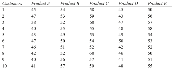
Use a randomized block design analysis to examine
(1) Whether the scores obtained for five different products differ significantly?
(2) Whether there is a significant difference between the average scores of the customers?
Take α = 0.05 as the level of significance for testing the hypotheses
Example 12.8
A company purchased four machines and installed them at four plants located at Raipur, Nagpur, Gwalior, and Indore. The machines are installed to produce one-metre long copper rods. The company provided training to four operators. These operators are employed on rotation basis at the four plants. After some time, the company received complaints about the variation in
the length of copper rods produced by the four machines. The company randomly selected some copper rods produced by four different operators from the four plants. Table 12.25 shows this randomly selected data in form of a two-way factorial design.
TABLE 12.25 Length of randomly selected copper rods arranged in a two-way factorial design

Take α = 0.05 and use the information given in Table 12.25 to perform a two-way ANOVA to determine whether there are significant differences in effects.
Solution The seven steps of hypothesis testing can be performed as below:
Step 1: Set null and alternative hypotheses
The null and alternative hypotheses can be stated as below:
Row effect: H0: All the row means are equal.
H1: All the row means are not equal.
Column effect: H0: All the column means are equal.
H1: All the column means are not equal.
Interaction effect: H0: Interaction effects are zero.
H1: Interaction effect is not zero (present).
Step 2: Determine the appropriate statistical test
F-test statistic in two-way ANOVA is given as
![]()
where MSC is the mean square column and MSE the mean square error
with c – 1, degrees of freedom for numerator and
rc (n – 1), degrees of freedom for denominator.
![]()
where MSR is the mean square row and MSE is the mean square error
with r – 1, degrees of freedom for numerator and
rc (n – 1), degrees of freedom for denominator.
![]()
where MSI is the mean square interaction and MSE the mean square error with (r – 1)(c – 1), degrees of freedom for numerator and
rc (n – 1) degrees of freedom for denominator.
Step 3: Set the level of significance
Level of significance α is taken as 0.05.
Step 4: Set the decision rule
For a given level of significance α, rules for acceptance or rejection of null hypothesis
Reject H0 if Fcalculated > Fcritical, otherwise, do not reject H0.
Step 5: Collect the sample data
The sample data is given in the Table 12.25.
Step 6: Analyse the data
The analysis is presented in the form of Minitab output (Figure 12.40) and partial MS Excel output (Figure 12.41)

Figure 12.40 Minitab output exhibiting ANOVA table and summary statistics for Example 12.8

Figure 12.41 Partial MS Excel output exhibiting ANOVA table for Example 12.8
Microsoft Office 2007, copyright © 2007 Microsoft Corporation.
Endnotes
1. Hair, J.F., M. Celsi, A. Money, P. Samouel and M. Page (2015), Essentials of Business Research, 3rd ed., p. 352. Taylor and Fransis.
2. Gray, C.D. and P.R. Kinner, (2012), IBM SPSS 19 Statistics Made Simple, p. 233, Psychology Press, an imprint of Taylor and Francis.
3. Pilla R. S., D. J. Kitska and C. Loader (2005), “Statistical Analysis of Modified Complete Randomized Designs: Applications to Chemo-Orientation Studies.” The Journal of Experimental Biology, 208: 1267–1276.
4. Holm, K. and N. J. Christman (1985). “Post Hoc Test Following Aanalysis of Variance,” Research in Nursing and Health, 8: 207–210.
5. Twisk, Jos W.R. (2013), Applied Longitudinal Data Analysis for Epidemiology, 2nd ed., p. 44. Cambridge University Press.
Step 7: Arrive at a statistical conclusion and business implication
At 95% confidence level, the critical value obtained from the table is F0.05, 2, 36 = 3.26, F0.05, 3, 36 = 2.87 and F0.05, 6, 36 = 2.36.
The calculated value of F for rows is 10.22. This is greater than the tabular value (3.26) and falls in the rejection region. Hence, the null hypothesis is rejected and alternative hypothesis is accepted.
The calculated value of F for columns is 1.05. This is less than the tabular value (2.87) and falls in the acceptance region. Hence, the null hypothesis is accepted and alternative hypothesis is rejected.
Calculated value of F for interaction is 5.25. This is greater than the tabular value (2.36) and falls in the rejection region. Hence, null hypothesis is rejected and alternative hypothesis is accepted.
The result indicates that there is a significant difference in length of the copper rods with respect to operators. The plant-wise difference in the length of copper rods produced is not found to be significant. Additionally, interaction between plants and operators is also found to be significant. The significant interaction effect indicates that the combination of operators and plants results in difference in the average rod length. So, the management must focus on operators first to check the difference in the length. The combination of plant and operators must also be considered to control the differences in the length of the copper rods.
SUMMARY |
An experimental design is the logical construction of the experiment to test hypotheses in which researcher either controls or manipulates one or more variables. Analysis of variance or ANOVA is a technique of testing a hypothesis about the significant difference in several population means. In analysis of variance (one-way classification), the total variation in the sample data can be divided into two components, namely variance between the samples and variance within the samples. Variance between the samples is attributed to the difference among the sample means. This variance is due to some assignable causes. One-way ANOVA is used to analyse the data from completely randomized designs.
Like completely randomized design, randomized block design also focuses on one independent variable of interest (treatment variable). Additionally, in randomized block design, we also include one more variable referred to as “blocking variable.” This blocking variable is used to control the confounding variable. Confounding variables are not being controlled by the researcher but can have an impact on the outcome of the treatment being studied. In case of a randomized block design, variation within the samples can be partitioned in two parts: unwanted variance attributed to difference between block means (block sum of square) (SSR); variance attributed to random error sum of squares errors) (SSE).
In some real-life situations, a researcher has to explore two or more treatments simultaneously. This type of experimental design is referred to as factorial design. In a factorial design, two or more treatment variables are studied simultaneously. Factorial design provides a platform to analyse both the treatment variables simultaneously at the same time in one experimental design. In a factorial design, a researcher can control the effect of multiple treatment variables. In addition, factorial design provides an opportunity to study the interaction effect of two treatment variables. The total sum of squares consists of four parts: SSC (sum of squares between columns), SSR (sum of squares between rows), SSI (sum of squares interaction), and SSE (sum of squares of errors).
Key terms |
Analysis of variance, 313
Classification variable, 313
Completely randomized design, 313
Dependent variable, 313
Experimental design, 313
Experimental units, 313
Factor, 313
Factorial design, 335
Independent variable, 312
Randomized block design, 335
Treatment variable, 312
notes |
- 1. www.tatamotors.com/our_world/profile.php, accessed August 2008.
Discussion questions |
- 1. Explain the concept of using experimental designs for hypothesis testing.
- 2. Define the following terms:
- Independent variable
- Treatment variable
- Classification variable
- Experimental units
- Dependent variable
- 3. What do you understand by ANOVA? What are the major assumptions of ANOVA?
- 4. What is the concept of completely randomized design and under what circumstances can we use completely randomized design for hypothesis testing?
- 5. Explain the procedure for calculating SSC (sum of squares between columns) and SSE (sum of squares within samples) in a completely randomized design.
- 6. Discuss the concept of randomized block design? Under what circumstances can we adopt randomized block design? Explain your answer in light of blocking variable and confounding variable.
- 7. Explain the procedure of calculating SSC (sum of squares between columns), SSR(sum of squares between rows), and SSE (sum of squares of errors) in a randomized block design.
- 8. Explain the difference between completely randomized design and randomized block design.
- 9. What do you understand by factorial design? Explain the concept of interaction in a factorial design.
- 10. Explain the procedure of calculating SSC (sum of squares between columns), SSR (sum of squares between rows), SSI (sum of squares interaction), and SSE (sum of squares of errors).
Numerical problems |
- 1. There are four cement companies A, B, C, and D in Chhattisgarh. Company “A” is facing a problem of high employee turnover. The personnel manager of this company believes that the low job satisfaction levels of employees may be one of the reasons for the high employee turnover. He has decided to compare the job satisfaction levels of the employees of his plant with those of the three other plants. He has used a questionnaire with 10 questions on a Likert rating scale of 1 to 5. The maximum scores that can be obtained is 50 and the minimum score is 10. The personnel manager has taken a random sample of 10 employees from each of the organizations with the help of a professional research organization. The scores obtained by the employees are given in the table below.

Use one-way ANOVA to analyse the significant difference in the job satisfaction scores. Take 99% as the confidence level.
- 2. A company has launched a new brand of soap Brand 1 in the market. Three different brands of three different companies already exist in the market. The company wants to know the consumer preference for these four brands. The company has randomly selected 10 consumers of each of the four brands and used a 1 to 4 rating scale, with 1 being the minimum and 4 being the maximum. The scores obtained are tabulated below:

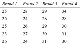
Use one-way ANOVA to analyse the significant difference in the consumer preference scores. Take 95% as the confidence level.
- 3. A consumer durable company located at New Delhi has launched a new advertisement campaign for a product. The company wants to estimate the impact of this campaign on different classes of consumers. For the same purpose, the company has divided consumer groups into three classes based on occupations. These are service class, business class, and consultants. For measuring the impact of the advertisement campaign, the company has used a questionnaire, which consists of 10 questions, on a 1 to 7 rating scale with 1 being minimum and 7 being maximum. The company has randomly selected 8 subjects (respondents) from each of the classes. So, a subject can score a minimum of 10 and maximum of 70. The scores obtained from the three classes of consumers are given below:
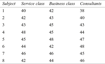
Use one-way ANOVA to determine the significant difference in the mean scores obtained by different consumers. Assume α = 0.05
- 4. A company has employed five different machines with five different operators working on it turn-by-turn. The table given below shows the number of units produced on randomly selected days by five machines with the concerned operator working on it:
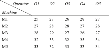
Use a randomized block design analysis to examine:
- (1) Whether the operators significantly differ in performance?
- (2) Whether there is a significant difference between the machines?
Take 90% as the confidence level.
- 5. A woolen threads manufacturer recently purchased three new machines. The company wants to measure the performance of these three machines at three different temperatures (in terms of unit production per day). The following table depicts the performance of the three machines at three different temperatures on randomly selected days:

Use a randomized block design analysis to examine:
- (1) Whether the machines are significantly different in terms of performance?
- (2) Whether there is a significant difference between the three different temperatures in terms of production?
Take 95% as the confidence level.
- 6. A company wants to ascertain the month wise productivity of its salesmen. The sales volume generated by five randomly selected salesmen in the first five months is given in the following table:

Use a randomized block design analysis to examine:
- (1) Whether the salesmen are significantly different in terms of performance?
- (2) Whether there is a significant difference between five months in terms of production?
Take 90% as the confidence level.
- 7. A company wants to measure the satisfaction level of consumers for a particular product. For this purpose, the company has selected respondents belonging to four age groups and asked a simple question, “Are you satisfied with this product?” Respondents were also classified into four regions. On the basis of four different age groups and regions, 48 customers were randomly selected. The company used a nine-point rating scale. The data given below represents the responses of the consumers:

Employ two-way ANOVA to determine whether there are any significant differences in effects. Take α = 0.05.
- 8. A water purifier company wants to launch a new model of its popular product. The company has divided its potential customers into three categories, “middle class,” “upper-middle class,” and “upper class.” Potential customers are further divided among three states of India, “Gujarat,” “Delhi,” and “Punjab.” For determining the purchase intention of the potential randomly selected consumers, the company has used a simple question, “Does this new product appeal to you?” The questionnaire is administered to 36 randomly selected customers from different classes and states. The company has used a five-point rating scale. The table given below depicts the responses of these randomly selected potential consumers:
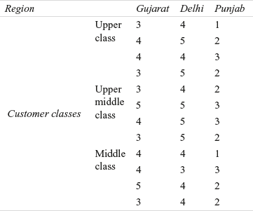
Employ a two-way ANOVA and determine whether there are any significant differences in effects. Take α = 0.01.
- 9. Black Pearl is a leading tyre manufacturing company in Pune. In the last 10 years, the company has achieved success in terms of branding, profitability, and market share. As a downside, the management has realized that the highly competitive and stressful environment has reduced its employee morale. For boosting employee morale, the company has opted for three methods: motivational speeches, meditation, and holidays with pay. The company researchers measure the success of the three-point programme after taking random samples from three departments, marketing, finance, and production. The researchers have used a questionnaire (10 questions) on a five-point rating scale. So, the maximum score can be 50 and minimum score can be 10. The scores obtained from 36 randomly selected employees are as shown in the given table:

Employ a two-way ANOVA and determine whether there are any significant differences in effects. Take α = 0.05.
Formulas |
Formulas for calculating SST (total sum of squares) and mean squares in one-way analysis of variance
SSC (sum of squares between columns) = ![]()
where k is the number of groups being compared, nj the number of observations in Group j, ![]() the sample mean of Group j, and
the sample mean of Group j, and ![]() the grand mean.
the grand mean.
and MSC (mean square) = ![]()
where SSC is the sum of squares between columns and k –1 the degrees of freedom (number of samples –1).
SSE (sum of squares within samples) = ![]()
where xij is the ith observation in Group j, ![]() the sample mean of Group j, k the number of groups being compared, and n the total number of observations in all the groups.
the sample mean of Group j, k the number of groups being compared, and n the total number of observations in all the groups.
and MSE (mean square) = ![]()
where SSE is the sum of squares within columns, and n – k the degrees of freedom (total number of observations–number of samples).
SST (total sum of squares) = ![]()
where xij is the ith observation in Group j, ![]() the grand mean, k the number of groups being compared, and n the total number of observations in all the groups.
the grand mean, k the number of groups being compared, and n the total number of observations in all the groups.
and MST (mean square) = ![]()
where SST is the sum of squares within columns and n – 1 the degrees of freedom (number of observations – 1)
F-test statistic in one-way ANOVA
![]()
where MSC is the mean square column and MSE the mean square error.
Formulas for calculating SST (total sum of squares) and mean squares in a randomized block design
SSC (sum of squares between columns) = ![]()
where r is the number of treatment levels (columns), n the number of observations in each treatment level (number of rows), ![]() the sample mean of Group j, and
the sample mean of Group j, and ![]() the grand mean.
the grand mean.
and MSC (mean square) = ![]()
where SSC is the sum of squares between columns and c – 1 the degrees of freedom (number of columns–1).
SSR (sum of squares between rows) = ![]()
where c is the number of treatment levels (columns), r the number of observations in each treatment level (number of rows), ![]() the sample mean of Group i (row means), and
the sample mean of Group i (row means), and ![]() the grand mean.
the grand mean.
and MSR (mean square) = ![]()
where SSE is the sum of squares within columns and r – 1 the degrees of freedom (Number of rows – 1).
SSE (sum of squares of errors) = ![]()
where c is the number of treatment levels (columns), r the number of observations in each treatment level (number of rows) ![]() the sample mean of Group i (Row means),
the sample mean of Group i (Row means),![]() the sample mean of Group j, xij the ith observation in Group j, and
the sample mean of Group j, xij the ith observation in Group j, and ![]() the grand mean.
the grand mean.
and MSE (mean square) = ![]()
where SSE is the sum of squares of errors and n – r – c + 1 = (c –1)(r –1) the degrees of freedom (number of observations – number of columns – number of rows + 1). Here, rc = n = number of observations.
F-test statistic in randomized block design
![]()
where MSC is the mean square column and MSE the mean square error.
with c – 1, degrees of freedom for numerator and
n – r – c + 1 = (c –1)(r – 1), degrees of freedom for denominator.
and ![]()
where MSR is the mean square row and MSE the mean square error.
with r – 1, degrees of freedom for numerator and
n – r – c + 1 = (c – 1)(r – 1) degrees of freedom for denominator.
Formulas for calculating SST (total sum of squares) and mean squares in a factorial design (two-way analysis of variance)
SSC (sum of squares between columns) = ![]()
where c is the number of column treatments, r the number of row treatments, n the number of observations in each cell, ![]() the sample mean of Group j, and
the sample mean of Group j, and ![]() the grand mean.
the grand mean.
and MSC (mean square) = ![]()
where SSC is the sum of squares between columns and c – 1 the degrees of freedom (number of columns –1).
SSR (sum of squares between rows) = ![]()
where c is the number of column treatments, r the number of row treatments, n the number of observations in each cell, ![]() the sample mean of Group i (row means), and
the sample mean of Group i (row means), and ![]() the grand mean.
the grand mean.
and MSR (mean square) = ![]()
where SSR is the sum of squares between rows and r – 1 the degrees of freedom (Number of rows –1)
SSI (sum of squares interaction) = ![]()
where c is the number of column treatments, r the number of row treatments, n the number of observations in each cell, ![]() the sample mean of Group i (row means),
the sample mean of Group i (row means), ![]() the sample mean of Group j (column means),
the sample mean of Group j (column means), ![]() the mean of the cell corresponding to ith row and jth column (cell mean), and
the mean of the cell corresponding to ith row and jth column (cell mean), and ![]() the grand mean
the grand mean
and MSE (mean square) = ![]()
where SSE is the sum of squares of errors and (r – 1)(c – 1) the degrees of freedom.
SSE (sum of squares errors) = ![]()
where c is the number of column treatments, r the number of row treatments, n the number of observations in each cell, xijk the individual observation, and ![]() the mean of the cell corresponding to ith row and jth column (cell mean)
the mean of the cell corresponding to ith row and jth column (cell mean)
and MSE (mean square) = ![]()
where SSE is the sum of squares of errors and rc (n – 1) is the degrees of freedom.
SST (total sum of squares) = ![]()
where c is the number of column treatments, r the number of row treatments, n the number of observations in each cell, xijk the individual observation, and ![]() the grand mean
the grand mean
and MST (mean square) = ![]()
where SST is the total sum of square and N – 1 the degrees of freedom (total number of observations – 1).
F-test statistic in two-way ANOVA
![]()
where MSC is the mean square column and MSE the mean square error
with c – 1, degrees of freedom for numerator
rc (n – 1) degrees of freedom for denominator.
![]()
where MSR is the mean square row and MSE the mean square error.
with r – 1 degrees of freedom for numerator
rc (n – 1) degrees of freedom for denominator.
![]()
where MSI is the mean square interaction and MSE the mean square error
with (r – 1)(c – 1) degrees of freedom for numerator and
rc (n – 1) degrees of freedom for denominator.
For a given level of significance α, the rules for acceptance or rejection of null hypothesis are as follows
Reject H0, if Fcalculated > Fcritical, otherwise do not reject H0.
Case study |
Case 12: Tyre Industry in India: A History of Over 75 Years
Introduction
The Indian government has been placing high emphasis on the building of infrastructure in the country. This has given a tremendous fillip to the development of road infrastructure and transport. After liberalization, there has been a remarkable increase in the numbers of vehicles on Indian roads. As a direct result of this, a heavy demand for tyres has been forecast in the near future. Indian tyre manufacturing companies have started re-engineering their businesses and are looking at strategic tie-ups worldwide to meet this demand.1 Table 12.01 shows the market segmentation for different categories of tyres.
Table 12.01 Market segmentation for different categories of tyres
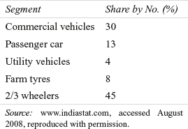
Major Players in the Market
MRF Ltd, Apollo Tyres Ltd, Ceat Ltd, JK Industries Ltd, GoodYear, Dunlop, etc. are some of the major players in the market. MRF Ltd is the leader in the market. The company is involved in the manufacturing, distribution, and the sales of tyres, tubes, and flaps for various vehicles. CEAT, established in 1958, is a part of the PRG group. CEAT is also a key player in the market and offers a wide range of tyres for almost all segments like heavy-duty trucks and buses, light commercial vehicles, earthmovers, forklifts, tractors, trailers, cars, motorcycles, and scooters, etc.
Apollo Tyres Ltd is also a dominant player in the truck, bus, and light commercial vehicle categories. In January 2008, the company announced an investment of Rs 12,000 million to set up a passenger car radial plant in Hungary to cater to the needs of the European and the North American market. It acquired Dunlop Tyre International along with its subsidiaries in Zimbabwe and the UK in April 20061. Apollo Tyres CMD, Mr Onkar Singh Kanwar, optimistically stated, “We believe that alliances offer the power of many companies working together for the benefit of the customer. This ultimately is for the greater good of the market and the individual companies.”2
JK Industries Ltd is the pioneer in launching radial tyres in India. Radial tyres cost 30% more but are technologically superior to conventional tyres. JK Tyres is the key player in the four-wheeler tyre market. In 1922, Goodyear tyre and rubber company Akron, Ohio, USA, entered the Indian market. Goodyear India has pioneered the introduction of tubeless radial tyres in the passenger car segment. Dunlop India Ltd is also a leading player in the market.
Worry Over Chinese Imports
Between April and December 2006, 550,000 trucks and bus tyres were imported from China when compared to just over 3 lakh units during the financial year 2005–2006. The increase in imports of low-priced tyres from China has become a sore point for Indian tyre manufacturers. Indian manufacturers are relying on the superior quality of Indian tyres to fight this battle. Mr Arun K. Bajoria, President, JK Tyre and Industries Ltd argued, “The quality of an Indian tyre and Chinese tyre cannot be compared. Indian tyres are exported to around 80 countries around the world and we have no complaints from anywhere on the quality.”3
With world class products under its stable, Indian tyre companies are getting ready to cater to an estimated demand of 22 million units of car and jeep tyres; 57 million units of two-wheelers tyres; 6.5 million units of LCV tyres; 17 million units of HCV tyres by 2014–2015.4
Let us assume that a researcher wants to compare the mean net sales of four leading companies Apollo Tyres Ltd, Ceat Ltd, JK Industries Ltd and MRF Ltd. The researcher is unable to access the complete net sales data of these companies and has taken a random sample of net sales for six quarters of the four companies taken for the study. Table 12.02 shows the net sales (in million rupees) of four leading tyre manufacturers in randomly selected quarters. Apply techniques presented in this chapter to find out whether:
Table 12.02 Net sales of four leading tyre manufacturers for six randomly selected quarters
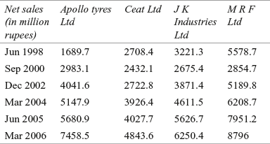
Source: Prowess (V. 3.1), Centre for Monitoring Indian Economy Pvt. Ltd, Mumbai, accessed August 2008, reproduced with permission.
- 1. The companies significantly differ in performance?
- 2. There is a significant difference between the quarterly sales of these companies?
notes |
- 1. Prowess (V. 3.1), Centre for Monitoring Indian Economy Pvt. Ltd, Mumbai, accessed August 2008, reproduced with permission.
- 2. www.tribuneindia.com/2003/200330901/biz.htm, accessed August 2008.
- 3. www.thehindubusinessline.com/2007/07/20/stories/2007072050461400.htm, accessed August 2008.
- 4. www.indiastat.com, accessed August 2008, reproduced with permission.