
Chapter 18
Factor Analysis and Cluster Analysis
Learning Objectives
Upon completion of this chapter, you will be able to:
- Understand the concept and application of factor analysis
- Interpret the factor analysis output obtained from the statistical software
- Use Minitab and SPSS to perform factor analysis
- Understand the concept and application of cluster analysis
- Interpret the cluster analysis output obtained from the statistical software
- Use SPSS to perform cluster analysis
RESEARCH IN ACTION: BATA INDIA LTD
In India, a large population demands a large shoe market, and the demand for footwear is continuously increasing. In the year 2000–2001, the demand for footwear was 900 million pairs, which is estimated to increase to 2290 million pairs by 2014–2015. In the time span of 2009–2010 to 2014–2015, the market is estimated to grow with a market growth rate of 7.5%. Despite this rosy scenario, market is highly segmented in favour of the informal market. Organized market has only 18% market share, whereas 82% of the market share is catered by the unorganized market. The footwear market is also diversified with respect to product variation. In the casuals, sports, formulas, and performance categories, footwear products occupy 53%, 32%, 7%, and 8% of the market share, respectively. Low-priced, medium-priced, and high-priced products occupy 65%, 32%, and 3% of the market share and leather, rubber/PVC, and canvas footwear occupy 10%, 35%, and 55% of the market share, respectively. Bata India, Liberty Shoe, Lakhani India, Nikhil Footwear, Graziella Shoes, Mirza Tanners, Relaxo Footwear, Performance Shoes, and so on are some of the leading players of the market.1
Bata India Ltd is the largest retailer and leading manufacturer of the footwear products in India and is a part of the Bata Shoe Organization. It was incorporated in 1931 as Bata Shoe Company Pvt. Ltd. The company initially started its business as a small operation in Konnagar in 1932. In January 1934, the company laid a foundation stone for the first building of Bata’s operation—now called the Bata. The company went public in 1973 when it changed its name to Bata India Ltd. With a wide retailer network of 1250 stores all over the country, today Bata India has established itself as India’s largest footwear retailer.2 Table 18.1 presents sales and profit after tax (in million rupees) of Bata India Ltd from 1994–1995 to 2008–2009.
Table 18.1 Sales and profit after tax (in million rupees) of Bata India Ltd from 1994–1995 to 2008–2009

Bata India Ltd, the largest shoe company in India, is overhauling its retail strategy to cope with the new dynamics of the marketplace after the centre opened up the segment to foreign single-brand stores. The company has taken a decision to be more visible in shopping malls, open up to franchisee models, and create the shop-in-shop experience in a multibranded store.3 The company has specific objectives to open showrooms in malls to cater the requirement of modern India. If a company wants to determine the features of an attractive showroom in the eyes of consumers and has appointed you as a researcher for conducting this research, with the help of literature and secondary data how will you determine the list of variables to be included in the study? If this list consists of some 70 statements generated from the literature, then how will you factorize these statements into a few factors?
In addition, if the company wants to group customers on some common attributes to present the different brands for the respective groups, then as a researcher, with the help of literature and secondary data, list down some of the common attributes on which the consumers can be clustered. Use the techniques of clustering presented in the chapter and cluster the customers on the basis of their preference for an attribute and then discuss how many cluster solutions will be an appropriate solution. Chapter 18 presents some well-known techniques to answer this question. The chapter deals with some of the commonly used multivariate techniques in the field of business research.
18.1 FACTOR ANALYSIS
Factor analysis is a widely used multivariate technique in the field of business research. It has been observed that many new researchers are using this technique without understanding the prerequisites for using it. The following section focuses on the use and application of factor analysis in the field of business research.
18.1.1 Introduction
The techniques described in this chapter, namely, factor analysis, cluster analysis, multidimensional scaling, and correspondence analysis are often referred as ‘interdependence analysis.’ As different from the regression and discriminant analysis, in the factor analysis, there is no concept of predicting the dependent variables through the independent variables. The factor analysis is most widely applied to multivariate technique of research, especially in the field of social and behavioural sciences. The techniques described in this chapter (factor analysis, cluster analysis, and multidimensional scaling) mainly examine the systematic interdependence among the set of observed variables, and the researcher is mainly focused on determining the base of commonality among these variables.
The techniques described in this chapter, namely, factor analysis, cluster analysis, multidimensional scaling, and correspondence analysis are often referred as “interdependence analysis.”
18.1.2 Basic Concept of Using the Factor Analysis
The factor analysis is a proven analytical technique that has been studied extensively by statisticians, mathematicians, and research methodologists.1 It is a very useful technique of data reduction and summarization. The main focus of the factor analysis is to summarize the information contained in a large number of variables into a few small number of factors. Generally for conducting any kind of research, a researcher has to collect information for a large number of variables. These variables are generally gathered either from the literature or from the experience of a researcher or an executive provides it. Most of these variables are correlated and can be reduced into fewer factors.
The main focus of the factor analysis is to summarize the information contained in a large number of variables into a few small number of factors. Generally for conducting any kind of research, a researcher has to collect information for a large number of variables.
The factor analysis allows a researcher to group the variables into a number of factors based on the degree of correlation among the variables. For example, if a company wishes to examine the degree of satisfaction the consumers are deriving from a launch of a new product, then it can collect variables from different sources such as literature, experience of the company executives, and so on. In fact, the list of these variables may be sufficiently large because this is the discretion of a researcher to include a large number of variables in the research. These variables may then be factor analysed to identify the underlying construct in the data. The name of the new factor (group of correlated variables) or factors can be subjectively defined by the researcher, which can be used for further multivariate analysis (may be regression or discriminant analysis). Thus, the factor analysis is a statistical technique used to determine the prescribed number of uncorrelated factors, where each factor is obtained from a list of correlated variables. The factor analysis can be utilized to examine the underlying patterns or relationships for a large number of variables and to determine whether the information can be condensed or summarized into a smaller set of factors or components.2
The factor analysis allows a researcher to group the variables into a number of factors based on the degree of correlation among the variables.
18.1.3 Factor Analysis Model
It has already been discussed that factor analysis is a statistical technique used to transform the original correlated variables into a new set of uncorrelated variables. These different groups of uncorrelated variables are referred as factors. Each factor is a linear combination of correlated original variables. Mathematically, it can be expressed as
![]()
where Fi is the estimate of the ith factor, ai the weights or factor score coefficients, and n the number of variables.
It is important to note that for forming a factor F1, each variable Xi, which is correlated with other variables, shares some variance with these other variables. This is referred as communality in the factor analysis.
The variable Xi may then be correlated with another group of variables to form another factor F2. It may be possible that another group of variables may not be significantly correlated with the variables, which formed Factor F1. This situation is explained in Figure 18.1.

Figure 18.1 Joining of various variables to form different factors
From Figure 18.1, it can be seen that Variable X1 is highly correlated with Variables X2, X3, and X4 to form Factor F1. It also clearly shows that Variable X1 is correlated with Variables X5 and X6 to form Factor F2. However, Variables X5 and X6 may not be correlated with Variables X2, X3, and X4. The covariance among the variables can be explained by a small number of common factors and the unique factor for each variable. Such Variable Xi may then be defined as
![]()
where Xi is the ith standardized variable, Aij the standardized multiple regression coefficient of Variable Xi on common Factor j, F the common factor, Vi the standardized regression coefficient of Variable Xi on Ui, Ui the unique factor in Xi, and m the number of common factors.
18.1.4 Some Basic Terms Used in the Factor Analysis
The following is the list of some basic terms frequently used in the factor analysis:
Correlation matrix: It is a simple correlation matrix of all the pairs of variables included in the factor analysis. It shows a simple correlation (r) between all the possible pairs of variables included in the analysis. In correlation matrix, the diagonal element is always equal to one, which indicates the correlation of any variable with the same variable.
Kaiser-Meyer-Olkin (KMO) measure of sampling adequacy: This statistic shows the proportion of variance, for variables included in the study is the common variance. In other words, this is the common variance, attributed to the underlying factors. A high value of this statistic (from 0.5 to 1) indicates the appropriateness of the factor analysis for the data in hand, whereas a low value of statistic (below 0.5) indicates the inappropriateness of the factor analysis.
Bartlett’s test of sphericity: This statistic tests the hypothesis whether the population correlation matrix is an identity matrix. This is important to note that with an identity matrix, the factor analysis is meaningless. Using significance level, the degree of relationship among the variables can be identified. A value less than 0.05 indicates that the data in hand do not produce an identity matrix. This means that there exists a significant relationship among the variables, taken for the factor analysis.
Communality: It indicates the amount of variance a variable shares with all other variables taken for the study.
Eigenvalue: It indicates the proportion of variance explained by each factor.
Percentage of variance: It gives the percentage of variance that can be attributed to each specific factor relative to the total variance in all the factors.
Scree plot: It is a plot of eigenvalues and component (factor) number according to the order of extraction. This plot is used to determine the optimal number of factors to be retained in the final solution.
Factor loadings: Also referred as factor–variable correlation. These are a simple correlation between the variables.
Factor matrix: Factor matrix table contains the factor loadings for each variable taken for the study on unrotated factors.
Factor score: It represents a subject’s combined response to various variables representing the factor.
Factor loading plot: It is a plot of original variables, which uses factor loadings as coordinates.
18.1.5 Process of Conducting the Factor Analysis
The factor analysis can be performed using the seven steps as shown in Figure 18.2: problem formulation, construction and examination of correlation matrix, selection of an appropriate factoring technique, a decision regarding the number of factors to be retained in the final solution, factor rotation for enhancing the interpretability of the solution, substantive interpretation, and check the model fit.
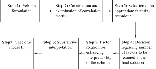
Figure 18.2 Seven steps involved in conducting the factor analysis
The following section describes a detailed discussion of these steps with the help of an example that is included in Step 1 as problem formulation.
18.1.5.1 Problem Formulation
The first step in conducting the factor analysis is to formulate the problem of the factor analysis. As discussed earlier, the main focus of the factor analysis is to reduce data. For this purpose, a researcher has to select a list of variables that will be converted into a new set of factors based on the common essence present in each of the variables. For selecting variables, a researcher can take the help of literature, past research, or use the experience of other researchers or executives. It is important to note that the variables should be measurable on an interval scale or a ratio scale. Another important aspect of the factor analysis is to determine the sample size, which will be used for the factor analysis. As a thumb rule, the sample size should be four or five times of the variable included in the factor analysis.
As a thumb rule, the sample size should be four or five times of the variable included in the factor analysis.
For understanding the factor analysis, let us consider an example of a garment company that wishes to assess the changing attitude of its customers towards a well-established product, in light of many competitors presence in the market. The company has taken a list of 25 loyal customers and administered a questionnaire to them. The questionnaire consists of seven statements, which were measured on a 9-point rating scale with 1 as strongly disagree and 9 strongly agree. The description of the seven statements used in the survey is given as follows:
X1: Price is a very important factor in purchasing.
X2: For marginal difference in price, quality cannot be compromised.
X3: Quality is OK, but competitor’s price of the same product cannot be ignored.
X4: Quality products are having a high degree of durability.
X5: With limited income, one can afford to spend only small portion for cloth purchase.
X6: In the present world of materialism and commercialization, people are evaluated on the basis of good appearance.
X7: By paying more if we can get good quality, why not to go for it.
Table 18.2 gives the rating scores obtained by different consumers for the seven statements described earlier.
Table 18.2 Rating scores obtained by different consumers for the seven statements to determine the changing consumer attitude

Figures 18.3(a)–18.3(m) shows the SPSS factor analysis output.
18.1.5.2 Construction and Examination of Correlation Matrix
The following discussion is based on the SPSS output, which is given in the form of Figures 18.3(a)–18.3(m). Figure 18.3(a) is a simple table that shows the descriptive statistics for the variables taken into study. In this figure, the second column shows the mean value for each item for 25 customers, the third column the degree of variability in scores for each item, and the fourth column the number of observations (sample size).
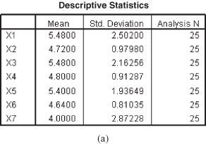

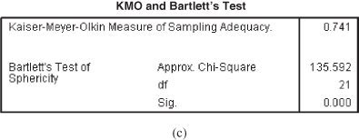

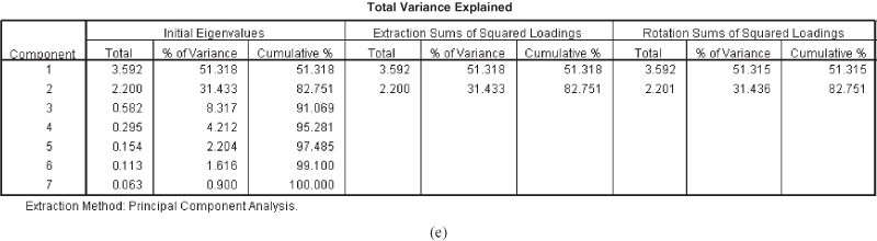
Figure 18.3 (a) Descriptive statistics, (b) Correlation matrix, (c) KMO and Bartlett’s test, (d) Communalities, (e) Total variance explained

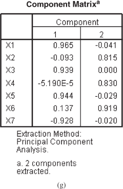
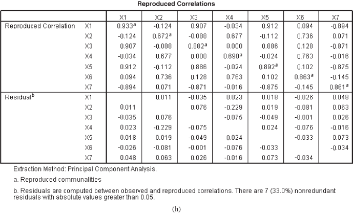
Figure 18.3 (f ) Scree plot, (g) Component matrix, (h) Reproduced correlations
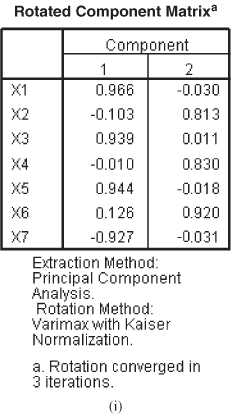
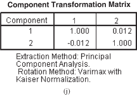


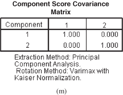
Figure 18.3 (i) Rotated component matrix, (j) Component transformation matrix (k) Component plot in rotated space, (l) Component score coefficient matrix, (m) Component score covariance matrix
Figure 18.3(b) is the SPSS-produced correlation matrix for the descriptor variables. This is the initial stage of the factor analysis, which gives some initial clues about the patterns of the factor analysis. It is important to note that for the appropriateness of the factor analysis, the variables must be correlated. If there is no correlation among the variables or if the degree of correlation among the variables is very low, then the appropriateness of the factor analysis will be under serious doubt. In the factor analysis, a researcher expects that some of the variables are highly correlated with each other to form a factor. Figure 18.3(b) shows that a few variables are relatively highly correlated with each other to form factors.
If there is no correlation among the variables or if the degree of correlation among the variables is very low, then the appropriateness of the factor analysis will be under serious doubt. In the factor analysis, a researcher expects that some of the variables are highly correlated with each other to form a factor.
Figure 18.3(c) shows two important statistics: the KMO measure of sampling adequacy and the Bartlett’s test of sphericity for judging the appropriateness of a factor model. KMO statistic compares the magnitude of the observed correlation coefficient with the magnitude of the partial correlation coefficient. As discussed earlier, a high value of this statistic (from 0.5 to 1) indicates the appropriateness of the factor analysis. Kaiser has presented the range as follows: statistic >0.9 is marvellous, >0.8 meritorious, >0.7 middling, >0.6 mediocre, >0.5 miserable, and <0.5 unacceptable. The figure shows that KMO statistic is computed as 0.741, which indicates the value in the acceptance region of the factor analysis model.
Kaiser has presented the range as follows: statistic >0.9 is marvellous, >0.8 meritorious, >0.7 middling, >0.6 mediocre, >0.5 miserable, and <0.5 unacceptable.
Bartlett’s test of sphericity tests the hypothesis whether the population correlation matrix is an identity matrix. The existence of the identity matrix puts the correctness of the factor analysis under suspicion. Figure 18.3(c) shows that chi square statistic is 135.592 with 21 degrees of freedom. This value is significant at 0.01 level. Both the results, that is, the KMO statistic and Bartlett’s test of sphericity, indicate an appropriate factor analysis model.
Bartlett’s test of sphericity tests the hypothesis whether the population correlation matrix is an identity matrix. The existence of the identity matrix puts the correctness of the factor analysis under suspicion.
18.1.5.3 Selection of an Appropriate Factoring Technique
After deciding the appropriateness of the factor analysis model, an appropriate technique for analysing the data is determined. Most of the statistical software available these days present a variety of methods to analyse the data. The principal component method is the most commonly used method of data analysis in the factor analysis model. When the objective of the factor analysis is to summarize the information in a larger set of variables into fewer factors, the principal component analysis is used.3 The main focus of the principal component method is to transform a set of interrelated variables into a set of uncorrelated linear combinations of these variables. This method is applied when the primary focus of the factor analysis is to determine the minimum number of factors that attributes maximum variance in the data. The obtained factors are often referred as the principal components. Another important method is the principal axis factoring, which will be discussed in the following section. Apart from the principal component method, a variety of other methods are also available. Description of all these methods is beyond the scope of this book.
The main focus of the principal component method is to transform a set of interrelated variables into a set of uncorrelated linear combinations of these variables. This method is applied when the primary focus of the factor analysis is to determine the minimum number of factors that attributes maximum variance in the data.
Figure 18.3(d) shows the initial and extracted communalities. The communalities describe the amount of variance a variable shares with all other variables taken into study. From the figure, it can be seen that the initial communality value is equal to 1 (as can be seen, the unities are inserted in the diagonal of correlation matrix) for all the variables taken into the factor analysis model. The SPSS, by default, assigns a communality value of 1 to all the variables. The extracted communalities as shown in the third column of Figure 18.3(d) is the estimate of variance in each variable, which can be attributed to factors in the factor solution. Relatively small value of the communality suggests that the concerned variable is a misfit for the factor solution and can (should) be dropped out from the factor analysis.
The communalities describe the amount of variance a variable shares with all other variables taken into study.
Figure 18.3(e) presents the initial eigenvalues (total, % of variance, and cumulative %), extraction sums of squared loadings (total, % of variance, and cumulative %), and the rotation sums of squared loadings (total, % of variance, and cumulative %). In this figure, the “Total” column gives the amount of variance in the variable attributed to the concerned component or factor. The“% of variance” column indicates the percentage of variance accounted for by each specific factor or component. It is important to note that the total variance accounted for by all the seven factors is equal to 7. This is equivalent to the number of variables. The variance attributed to factor 1 is 3.592/7 × 100 = 51.31%. The total variance attributed to factor 2 is 2.200/7 × 100 = 31.43%. Similarly, the total variance attributed to all the factors can be computed. The second part of the figure is the extraction sums of squared loadings that gives information related to the extracted factors or components. If a researcher has adopted the “principal component method” as the method of analysis in a factor model, then the values will remain the same, as shown under the heading “initial eigenvalues.” As can be seen from the third part of the figure, rotation sums of squared loadings, the variance accounted for by the rotated factors or components is different from those indicated in the second column of extraction sums of squared loadings. It is important to note that for rotation sums of squared loadings, the cumulative percentage for the set of components (factors) will always remain the same.
% of variance indicates the percentage of variance accounted for by each specific factor or component.
- 18.1.5.4 Decision Regarding the Number of Factors to be Retained in the Final Solution
It is possible to have a number of factors as the number of variables available in the factor analysis. If this is the case, the rationale of applying factor analysis is questionable because the primary objective of the factor analysis is to summarize the information contained in the various variables into a few factors. For this purpose, the basic question in the mind of a researcher while applying factor analysis is that how many factors should be abstracted from the factor analysis. In their research paper “Evaluating the use of exploratory factor analysis in psychological research,” L.R. Fabrigar et al. have stated that determining how many factors to include in the model requires the researcher to balance the need for parsimony (i.e., a model with relatively few common factors) against the need for plausibility (i.e., a model with a sufficient number of common factors to adequately account for the correlations among the measured variables).4 A number of approaches are available to decide the number of factors to be retained in the factor analysis solution. In this section, we will focus on three commonly used criteria for determining the number of factors: eigenvalue criteria, Scree plot criteria, and percentage of variance criteria.
A number of approaches are available to decide the number of factors to be retained in the factor analysis solution.
Eigenvalue Criteria
An eigenvalue is the amount of variance in the variable taken for the study that is associated with a factor. According to the eigenvalue criteria, the factors having more than one eigenvalue are included in the model. A factor that has an eigenvalue of less than 1 is not better than a single variable because due to standardization each variable has a variance of 1.
An eigenvalue is the amount of variance in the variable taken for the study that is associated with a factor. According to eigenvalue criteria, the factors having more than one eigenvalue are included in the model.
Scree Plot Criteria
One of the most popular guides for determining how many factors should be retained in the factor analysis is the Scree test.5 Scree plot is a plot of the eigenvalues and component (factor) number according to the order of extraction [as shown in Figure 18.3(f)]. The shape of the plot is used to determine the optimum number of factors to be retained in the final solution. The objective of the Scree plot is to visually isolate an elbow, which can be defined as the point where the eigenvalues form a liner descending trend.6 For an appropriate factor analysis model, this plot looks like an intersection of two lines (Figure 18.4).
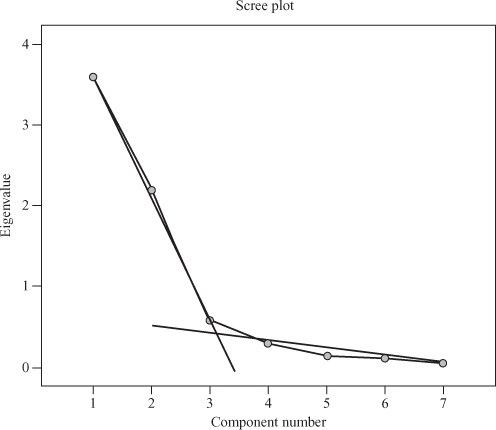
Figure 18.4 Scree plot shown as an intersection of two lines
Scree plot is a plot of the eigenvalues and component (factor) number according to the order of extraction.
Figure 18.5 clearly shows that the factors on the steep slope should be retained in the model and the factors on the shallow slope can be excluded from the model (as these factors contribute relatively little to the factor model).
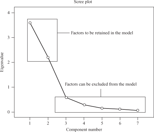
Figure 18.5 Scree plot indicating the number of factors to be retained in the model
Percentage of Variance Criteria
This approach is based on the concept of cumulative percentage of variance. The number of factors should be included in the model for which cumulative percentage of variance reaches a satisfactory level. Now there is a question that what should be that satisfactory level. However, the general recommendation is that the factors explaining 60%–70% of the variance should be retained in the model.
However, the general recommendation is that the factors explaining 60%–70% of the variance should be retained in the model.
Considering Figures 18.3(e) and 18.3(f), all the three approaches suggest that the number of factors to be extracted should be only two. According to the eigenvalue approach, only two factors have eigenvalues more than 1. The Scree plot for the problem in hand also shows that only two factors on the steep slope should be retained in the model. The cumulative percentage of variance for the first two factors is 82.751%, which is well within the prescribed limits, which is why only two factors must be retained in the final factor analysis solution. Above are some criteria; however, the number of factors to be retained is a highly subjective matter. The scope of interpretation can be enhanced by rotating the factors and will be described in the following section.
According to the eigenvalue approach, only two factors have eigenvalues more than 1. The Scree plot for the problem in hand also shows that only two factors on the steep slope should be retained in the model. The cumulative percentage of variance for the first two factors is 82.751%, which is well within the prescribed limits, which is why only two factors must be retained in the final factor analysis solution.
Figure 18.3(g) shows the component matrix table that presents the factor loading for each variable on unrotated factors (components). As can be seen from the figure, each value under the heading component (1 or 2) represents the correlation between the concerned variable and the unrotated factors. The values given under Factor 1 represent the correlation between the concerned variable and Factor 1, and the values given under Factor 2 represent the correlation between the concerned variable and Factor 2. From this figure, it can be seen that Variables X1, X3, X5, and X7 are relatively highly correlated (with values 0.965, 0.939, 0.944, and −0.928) with Factor 1, and Variables X2, X4, and X6 are relatively highly correlated with Factor 2 (with values 0.815, 0.830, and 0.919).
Figure 18.3(h) shows the reproduced correlation and residuals for the factor analysis solution. For an assumed appropriate factor analysis solution, the reproduced correlation shows the predicted pattern of relationship. The residuals are the difference between the predicted and observed values. If a factor analysis solution is good enough, then most of the residual values are small.
The residuals are the difference between the predicted and observed values. If a factor analysis solution is good enough, then most of the residual values are small.
- 18.1.5.5 Factor Rotation for Enhancing the Interpretability of the Solution
After selection of factors, the immediate step is to rotate the factors. The rotated simple structure solutions are often easy to interpret, whereas the originally unextracted (unrotated) factors are often difficult to interpret.7 A rotation is required because the original factor model may be mathematically correct but may be difficult in terms of interpretation. If various factors have a high loading on the same variable, then interpretation will be extremely difficult. Rotation solves this kind of interpretation difficulty. The main objective of rotation is to produce a relatively simple structure in which there may be a high factor loading on one factor and a low factor loading on all other factors
The main objective of rotation is to produce a relatively simple structure in which there may be a high factor loading on one factor and a low factor loading on all other factors.
. Similar to correlation, factor loading varies between +1 and −1 and indicates the degree of relationship between a particular factor and the particular variable. It is interesting to note that rotation never affects the communalities and the total variance explained [from Figure 18.3(e), it can be seen that after rotation, the cumulative percentage of variance is not changed (82.751%)].
A rotation is required because the original factor model may be mathematically correct but may be difficult in terms of interpretation.
Figure 18.6 shows asterisks on the unrotated factor lines, and Figure 18.7 shows asterisks on the rotated factor lines. If we compare both the figures, the rationale of rotation can be easily explained. Rotation enhances the interpretability in terms of association of factor loadings with the concerned factor. When compared with Figure 18.6, Figure 18.7 clearly explains the high factor loading on one factor and the low factor loading on all other factors.
Figure 18.6 Asterisks on the unrotated factor lines

Figure 18.7 Asterisks on the rotated factor lines
Rotation enhances the interpretability in terms of association of factor loadings with the concerned factor.
Figure 18.3(i) represents the rotated component matrix that is often referred as the ‘pattern matrix for oblique rotation.’ The columns in this figure represent the factor loading for each variable, for the concerned factor, after rotation. The figure clearly shows the interpretability importance of the rotation.
Earlier, the rotation was done manually by the researchers, whereas nowadays, a variety of statistical softwares present a variety of methods of rotation such as Varimax procedure, Quartimax procedure, Equamax procedure, Promax procedure, and so on. However, the different rotation procedures more or less reflect the same result about the data; by performing different procedures and later comparing the results of the different schemes, obtaining the ‘most interpretable’ solution will always be beneficial for researchers.
The widely applied method of rotation is the ‘Varimax procedure.’
The widely applied method of rotation is the ‘Varimax procedure.’ Although a number of rotation methods have been developed, varimax has been generally regarded as the best orthogonal rotation and is overwhelmingly the most widely used orthogonal rotation in psychological research.8 This section focuses on varimax procedure of rotation.
Nowadays, a variety of statistical software present a variety of methods of rotation such as Varimax procedure, Quartimax procedure, Equamax procedure, Promax procedure, and so on.
The rotation is often referred as ‘orthogonal rotation’ if the axes are maintained at right angles. Varimax procedure is an orthogonal rotation procedure. Orthogonal rotation generates the factors that are uncorrelated. On the other hand, in oblique rotation, axes are not rotated at right angle and the factors are correlated. If the factors are truly uncorrelated, orthogonal and oblique rotation produce nearly identical results.9
The rotation is often referred as ‘orthogonal rotation’ if the axes are maintained at right angles. Varimax procedure is an orthogonal rotation procedure.
The rotated factor matrix as shown in Figure 18.3(i) shows that the Variables X1, X3, X5, and X7 are having high loadings on Factor 1 and the Variables X2, X4, and X6 are having high loadings on Factor 2.
18.1.5.6 Substantive Interpretation
At this stage, there is a point to identify the factors with concerned variables as the constituents of the factor. Figure 18.3(k), as the component plot in rotated space, provides this opportunity. Before that, it is important to interpret Figure 18.3(j). Figure 18.3(j) shows the component transformation matrix. The component transformation matrix is used to construct the rotated factor matrix from the unrotated factor matrix by using a simple formula (unrotated factor loading × factor transformation matrix = rotated factor loadings). In the case in which off-diagonal elements are close to zero indicates a relatively smaller rotation and off-diagonal elements are large (greater than ±5) indicates a relatively larger rotation.
As described in the previous paragraph, Figure 18.3(k) is the component plot in rotated space. This plot is a pictorial representation of the factor loadings of the variables taken in the study on the first few factors. The variables near or on the axis show a high factor loading on the concerned factor. Figure 18.3(k) shows that the Variables X1, X3, X5, and X7 are highly loaded on Factor 1. It is interesting to see here that the Variable X7 has got the high negative value, and hence, it is in the opposite direction of the three Variables X1, X3, and X5. If a variable is not a part of any factor (neither close to horizontal axis nor close to vertical axis), then it should be treated as an undefined or a general factor. Similarly, the Variables X2, X4, and X6 have high factor loadings on Factor 2.
Factor 1 consists of Variables X1 (price is important), X3 (competitor’s price cannot be ignored), X5 (limited affordability), and X7 (get good quality by paying more). Negative factor loading value of Variable X7 on Factor 1 indicates that this segment of customers is more concerned about the price even at the cost for compromising quality. Hence, Factor 1 can be named as ‘Economy Seekers.’ Similarly, Factor 2 consists of Variables X2 (quality cannot be compromised), X4 (quality products are having a high degree of durability), and X6 (societal evaluation of an individual is based on quality products). Thus, Factor 2 can be named as ‘Quality seekers.’ After applying the factor analysis, the original seven variables are categorized into two factors economy seekers and quality seekers.
Figure 18.3(l) shows the component score coefficient matrix. For each subject, the factor score is calculated by multiplying the values of variable (can be obtained from Table 18.2) by factor score coefficients. For example, for Subject 1, factor score can be computed as follows:
For Factor 1:
(0.269) × (8) + (−0.030) × (4) + (0.261) × (7) + (−0.005) × (5) + (0.263) × (7) + (0.033) × (4) + (−0.258) × (2) = 4.211.
For Factor 2:
(−0.015) × (8) + (0.370) × (4) + (0.003) × (7) + (0.377) × (5) + (−0.010) × (7) × (0.418) × (4) + (−0.012) × (2) = 4.844.
Similarly, using the factor score coefficient, factor scores for other subjects can also be computed. Instead of all the original variables, the factor scores can be used in the subsequent multivariate analysis. Sometimes instead of computing a factor score, researchers select the substitute variable commonly known as surrogate variable by selecting some of the original variables for further multivariate analysis. It is important to note that a researcher can also select the variables on a discretionary basis. This means that on the basis of experience or literature or any other logical basis, if a researcher believes that the variable with a high factor loading is less important than the variable with a low factor loading, then he or she can select the relatively important variable with a low factor loading as the surrogate variable.
Sometimes instead of computing a factor score, researchers select the substitute variable commonly known as surrogate variable by selecting some of the original variables for further multivariate analysis.
18.1.5.7 Check the Model Fit
The last step in the factor analysis is to determine the fitness of the factor analysis model. In factor analysis, the factors are generated on the basis of observed correlation between the variables. The degree of correlation between the variables can be reproduced as shown in Figure 18.3(h). For an appropriate factor analysis solution, the difference between the reproduced and observed correlation should be small (less than 0.05). As can also be seen from Figure 18.3(h), only seven residuals are greater than 0.05, which indicates an appropriate factor analysis model.
For an appropriate factor analysis solution, the difference between the reproduced and observed correlation should be small (less than 0.05).
18.1.6 Using Minitab for the Factor Analysis
For conducting the factor analysis using Minitab, click Start/Multivariate/Factor Analysis. Factor Analysis dialogue box will appear on the screen (Figure 18.8). Place the variables taken for the study in the ‘Variables’ box. From ‘Method of Extraction’ select ‘Principal components.’ From ‘Type of Rotation’ select ‘Varimax’ and click on ‘Options’ box. Factor Analysis-Options dialogue box as shown in Figure 18.9 will appear on the screen. In this dialogue box, from ‘Matrix to Factor’ select ‘Correlation,’ from ‘Source of Matrix’ select ‘Compute from variables,’ and from ‘Loading for Initial Solution’ select ‘Compute from variables’ and click OK. Factor Analysis dialogue box will reappear on the screen. From this dialogue box select ‘Graphs.’ Factor Analysis-Graphs dialogue box will appear on the screen (Figure 18.10). Select all the four plots shown in this dialogue box as shown in Figure 18.10 and click OK. Factor Analysis dialogue box will reappear on the screen. From this dialogue box select ‘Results.’ Factor Analysis-Results dialogue box will appear on the screen (Figure 18.11). From this dialogue box select ‘Display of Results,’ ‘Loading and factor score coefficients’ and click OK. Factor Analysis dialogue box will reappear on the screen. From this dialogue box click OK. Minitab output in session window will appear on the screen (Figures 18.12–18.17).

Figure 18.8 Minitab Factor Analysis dialogue box

Figure 18.9 Minitab Factor Analysis-Options dialogue box
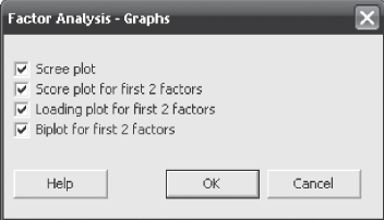
Figure 18.10 Minitab Factor Analysis-Graphs dialogue box

Figure 18.11 Minitab Factor Analysis-Results dialogue box
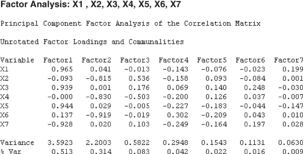
Figure 18.12 Partial Minitab output for garment company example (before rotation)

Figure 18.13 Partial Minitab output for garment company example (after rotation)

Figure 18.14 Minitab-produced Scree plot
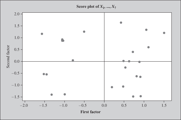
Figure 18.15 Minitab-produced factor score plot for the first two factors

Figure 18.16 Minitab-produced factor loading plot for the first two factors

Figure 18.17 Minitab-produced biplot for the first two factors
In the principal component method of extraction, if a researcher does not specify the ‘Number of factors to extract’ (as in our case), Minitab produces the number of factors equal to the number of variables in the data set. As can be seen from Figures 18.12 and 18.13, the number of factors extracted from Minitab is seven because we have taken seven variables for the study. Figures 18.14–18.17 are Minitab-produced Scree plot, factor score plot for the first two factors, factor loading plot for the first two factors, and biplot for the first two factors, respectively. Factor score plot (Figure 18.15) is a plot between the first factor scores and the second factor scores. This plot checks the assumption of normality and the status of outlier. When the data are normally distributed and no outlier is present, the points around zero are randomly distributed as shown in Figure 18.15. The factor loading plot (Figure 18.16) indicates information about the loading of the first two factors. The biplot shows the factor scores and loadings in one plot.
18.1.7 Using the SPSS for the Factor Analysis
For conducting the factor analysis using the SPSS, click Analyse/Data Reduction/Factor. Factor Analysis dialogue box will appear on the screen (Figure 18.18). From this dialogue box click ‘Descriptives.’ Factor Analysis: Descriptives dialogue box will appear on the screen (Figure 18.19). In this dialogue box, from ‘Statistics’ select ‘Univariate descriptives’ and ‘Initial solution.’ From ‘Correlation Matrix’ select ‘Coefficients,’ ‘Significance levels,’ ‘Determinant,’ ‘KMO and Bartlett’s test of sphericity,’ ‘Reproduced,’ and click Continue. Factor Analysis dialogue box will reappear on the screen. From this dialogue box, click Extraction. Factor Analysis: Extraction dialogue box will appear on the screen (Figure 18.20). In this dialogue box, from ‘Method’ select ‘Principal components’ and from ‘Display’ select ‘Unrotated factor solution’ and ‘Scree plot.’ Against ‘Extract’ specify ‘Eigenvalues greater than 1’ and click Continue. Factor Analysis dialogue box will reappear on the screen. In this dialogue box, click ‘Rotation.’ Factor Analysis: Rotation dialogue box will appear on the screen (Figure 18.21). In this dialogue box, from ‘Method’ select ‘Varimax’ and from ‘Display’ select ‘Rotated solution’ and ‘Loading plot(s)’ and click Continue. Factor Analysis dialogue box will reappear on the screen. From this dialogue box, click Scores. Factor Analysis: Factor Scores dialogue box will appear on the screen (Figure 18.22). In this dialogue box, click ‘Display factor score coefficient matrix’ and Continue. Factor Analysis dialogue box will reappear on the screen. From this dialogue box, click Options. Factor Analysis: Options dialogue box will appear on the screen (Figure 18.23). In this dialogue box, from ‘Missing Values’ select ‘Exclude cases listwise’ and click Continue. Factor Analysis dialogue box will reappear on the screen. From this dialogue box, click OK. The SPSS will produce the output as shown in Figures 18.3(a)–18.3(m).
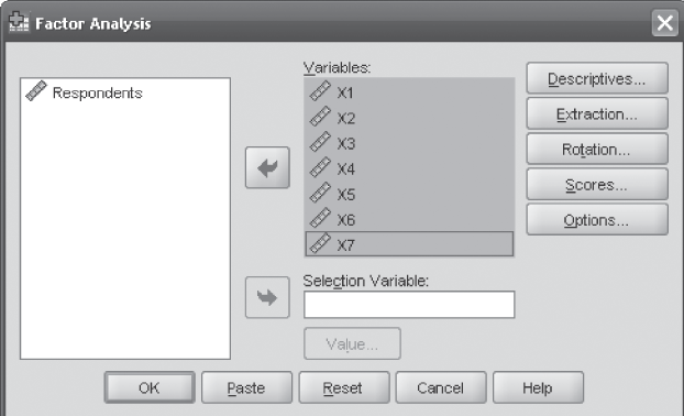
Figure 18.18 SPSS Factor Analysis dialogue box
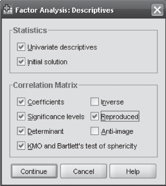
Figure 18.19 SPSS Factor Analysis: Descriptives dialogue box
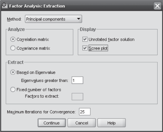
Figure 18.20 SPSS Factor Analysis: Extraction dialogue box

Figure 18.21 SPSS Factor Analysis: Rotation dialogue box
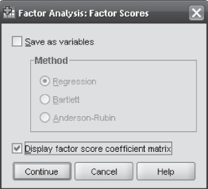
Figure 18.22 SPSS Factor Analysis: Factor Scores dialogue box
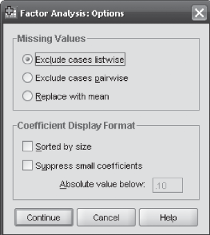
Figure 18.23 SPSS Factor Analysis: Options dialogue box
18.2 CLUSTER ANALYSIS
This section focuses on a popular multivariate technique known as cluster analysis. It deals with all important dimensions related to the application of cluster analysis. Use of SPSS output for explaining the concept will make its use very convenient for a researcher.
18.2.1 Introduction
In every field of the study, researchers or scientists or marketing executives will like to group the objects on the basis of some similarity. Specifically, in the field of marketing, mangers try to identify a similar group of customers, so that the marketing strategies can be chalked out for the concerned similar group of customers. These customers can be grouped or clustered on the basis of a variety of common features such as the benefits the consumers seek from the product, lifestyle of the consumers with special reference to its impact on their purchase behaviour, and so on. The main objective of the marketing executives is to find out a similar group of customers to develop products or services according to their specific need. Thus, the researchers or executives face a common problem in terms of availability of some scientific technique to group the objects on the basis of some similarity. Cluster analysis provides a solution to this kind of problem. It has become a common tool for the marketing researcher.10 In some aspects, the factor analysis and cluster analysis are similar. In both, a researcher tries to reduce a larger number of variables (in factor analysis) or cases (in cluster analysis) into a smaller number of factors (in factor analysis) or clusters (in cluster analysis) on the basis of some commonality that within-group members share with each other. However, the statistical procedure to do this and the interpretations are different in these two methods.
Specifically, in the field of marketing, mangers try to identify a similar group of customers, so that marketing strategies can be chalked out for the concerned similar group of customers. These customers can be grouped or clustered on the basis of a variety of common features such as the benefits the consumers seek from the product, lifestyle of the consumers with special reference to its impact on their purchase behaviour, and so on.
18.2.2 Basic Concept of Using the Cluster Analysis
Cluster analysis is a technique of grouping individuals or objects or cases into relatively homogeneous (similar) groups that are often referred as clusters. The subjects grouped within the cluster are similar to each other, and there is a dissimilarity between the clusters. In other words, we can say that the individuals or objects or cases when correlated with each other form a cluster. The main focus of the cluster analysis is to determine the number of mutually exclusive and collectively exhaustive clusters in the population, on the basis of similarity of profiles among the subjects. In the field of marketing, cluster analysis is mainly used in market segmentation, understanding purchase behaviour of the consumers, test marketing, and so on. A typical use of cluster analysis is to provide market segmentation by identifying subjects or individuals who have similar needs, lifestyles, or responses to marketing strategies.11 For example, in the process of launching a new product, the CEO of a company wants to group cities of the country on the basis of age group and education of the consumers. If a company has collected data from 15 customers of various cities, then a simple way to group the subjects is to plot the result on two variables, that is, age and education of the consumers. Figures 18.24(a) and 18.24(b) present two different situations: before clustering and after clustering. In most of the cases, the researchers or business executives find situations as explained in Figure 18.24(a). This is a situation when there is no clustering and the subjects are scattered with respect to the two variables: age and education. Figure 18.24(b) shows after clustering situation in which subjects join to form different clusters based on some similarity.
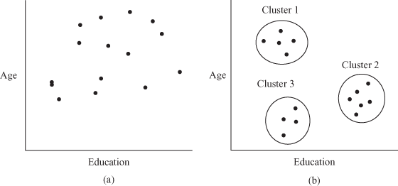
Figure 18.24 (a) Before clustering situation, (b) After clustering situation
Cluster analysis is a technique of grouping individuals or objects or cases into relatively homogeneous (similar) groups that are often referred as clusters. The subjects grouped within the cluster are similar to each other, and there is a dissimilarity between the clusters.
The main focus of the cluster analysis is to determine the number of mutually exclusive and collectively exhaustive clusters in the population, on the basis of similarity of profiles among the subjects.
18.2.3 Some Basic Terms Used in the Cluster Analysis
The following list presents some basic terms that are commonly used in the cluster analysis:
Agglomeration Schedule: It presents the information on how the subjects are clustered at each stage of the hierarchical cluster analysis.
Cluster Membership: It indicates the cluster to which each subject belongs according to the number of cluster requested by a researcher.
Icicle plot: It provides a graphical representation on how the subjects are joined at each step of the cluster analysis. This plot is interpreted from bottom to top.
Dendrogram: Also referred as tree diagram. It is a graphical representation of relative similarities between the subjects. It is interpreted from left to right in which the cluster distances are rescaled, so that the plot shows the range from 0 to 25.
18.2.4 Process of Conducting the Cluster Analysis
The process of conducting the cluster analysis involves six steps as shown in Figure 18.25: problem formulation, choice of an appropriate proximity or similarity measure, selection of an appropriate clustering technique, a decision regarding the number of clusters to be retained in the final solution, substantive interpretation, and check the model fit.
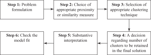
Figure 18.25 Six steps involved in conducting the cluster analysis
The following section describes a detailed discussion of these steps with the help of an example that is included in Step 1 as problem formulation.
18.2.4.1 Problem Formulation
The first and most important step in the cluster analysis is to formulate the problem properly in terms of properly defining the variables on which the clustering procedure is to be performed. For understanding the procedure of conducting the cluster analysis, let us formulate a problem. A famous motorbike company wants to launch a new model of motorbike with some additional features. Before launching the product to an entire country, the company has to test market it in select cities. The company is well aware that the majority of the target consumer group consists of urban youth (aged below 45). For understanding the future purchase behaviour of the consumers, the company administered a questionnaire to the potential future customers. The questionnaire consists of seven statements that were measured on a 9-point rating scale with 1 as strongly disagree and 9 as strongly agree. The description of the seven statements used in the survey is given as follows:
X1: I am trying very hard to understand the loan schemes offered by different banks to purchase the product when it will be coming in the market.
X2: I am still in confusion whether to sell my old bike or not.
X3: My old bike is old fashioned; I want to get rid of it.
X4: My company has promised that it will be releasing a much awaited new incentive scheme; purchase of a new model is based on this factor.
X5: I will not wait for the product’s performance in the market, I know the company is reputed and will certainly launch a quality product.
X6: Companies always claim high about its product, let the product come in the market only then I will be taking any decision about the purchase.
X7: I want to purchase a new bike but my kids are growing up and are demanding to purchase a car instead of a bike, which I already have.
Table 18.3 gives the rating scores obtained by different potential consumers for the seven statements, as described earlier, to determine the future purchase behaviour.
Table 18.3 Rating scores obtained by different consumers for the seven statements to determine the future purchase behaviour
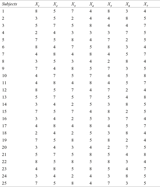
For explaining the procedure of conducting cluster analysis, only 25 subjects are selected, but in practice, the cluster analysis is performed on more than or equal to 100 subjects.
18.2.4.2 Choice of an Appropriate Proximity or Similarity Measure
It has already been discussed in the beginning of the chapter that in the cluster analysis, the subjects are grouped on the basis of similarity or commonality. Thus, there is a need to have a measurement of similarity method by which similarity between the subjects can be identified, to group similar subjects in a cluster.
In the cluster analysis, the subjects are grouped on the basis of similarity or commonality. Thus, there is a need to have a measurement of similarity method by which similarity between the subjects can be identified, to group similar subjects in a cluster.
The method that is widely used for measuring the similarity is the Euclidean distance or its square. The Euclidean distance is the square root of the sum of squared differences between the values for each variable. The squared Euclidean distance is the sum of squared differences between the values for each variable. This distance measure is used for the interval data. Varieties of other measures are also available, but this section will mainly focus on the squared Euclidean distance method. The Euclidean distance measure also has one disadvantage in terms of varying result with varying units. This disadvantage can be overcome by expressing all the variables in a standardized form with a mean value of zero and standard deviation one.
The method that is widely used for measuring the similarity is the Euclidean distance or its square. The Euclidean distance is the square root of the sum of squared differences between the values for each variable. The squared Euclidean distance is the sum of squared differences between the values for each variable.
18.2.4.3 Selection of an Appropriate Clustering Technique
There are two approaches of clustering: hierarchical clustering approach and non-hierarchical clustering approach. Hierarchical clustering starts with all the subjects in one cluster and then dividing and subdividing them till all the subjects occupy their own single-subject cluster. As different from hierarchical clustering, non-hierarchical clustering allows subjects to leave one cluster and join another in the cluster forming process if by doing so the overall clustering criterion will be improved. The various clustering procedures are shown in Figure 18.26.

Figure 18.26 Different methods of clustering
There are two approaches of clustering: hierarchical clustering approach and non-hierarchical clustering approach. Hierarchical clustering starts with all the subjects in one cluster and then dividing and subdividing them till all the subjects occupy their own single subject cluster. As different from hierarchical clustering, non-hierarchical clustering allows subjects to leave one cluster and join another in the cluster forming process if by doing so the overall clustering criterion will be improved.
In the hierarchical clustering method, various approaches are available to cluster the subjects in different clusters. It can mainly be divided into two categories: agglomerative and divisive. In agglomerative clustering, initially each subject occupies a separate cluster. In this process of clustering, clusters are created by grouping the subjects into bigger and bigger clusters until all the subjects join a single cluster. In divisive clustering, as clear from the name itself, initially all the subjects or members are grouped into a single cluster and then the clusters are divided until each subject occupies a single cluster.
The hierarchical clustering method can mainly be divided into two categories: agglomerative and divisive.
As discussed, varieties of clustering methods are available, but in the field of marketing, the agglomerative methods are widely used. From Figure 18.26, we can see that agglomerative methods are categorized into linkage method, variance method, and centroid method. Linkage method is based on how the distance between the two clusters is defined. On the basis of the procedure of measuring the distance, it can be categorized into three categories: single linkage method, complete linkage method, and average linkage method.
Agglomerative methods are categorized into linkage method, variance method, and centroid method. Linkage method is based on how the distance between the two clusters is defined. On the basis of the procedure of measuring the distance, it can be categorized into three categories: single linkage method, complete linkage method, and average linkage method.
The single linkage method also referred as the nearest neighbour approach is based on the principle of the shortest distance. This method measures the shortest distance between the two individual subjects and places them into the first cluster. Then on the basis of the next shortest distance, either the third subject joins the first two or a new subject cluster is constituted [Figure 18.27(a)]. This process continues until all the subjects become a member of one cluster. The complete linkage method also referred as the farthest neighbour approach is based on the principle of the longest distance. This method is similar to the single linkage method except the measurement pattern in which the distance between the two clusters is measured as the distance between their two furthest points [Figure 18.27(b)]. As the name indicates, in the average linkage method, the distance between the two clusters is defined in terms of the average of the distance between all pairs of the subjects, in which one subject of the pair is from each of the clusters [Figure 18.27(c)]. This method is preferred over the single linkage and complete linkage methods because it avoids taking two extreme members while taking the distance between the two clusters. In fact, this method considers all the members of the cluster rather than the two extreme members of the clusters.
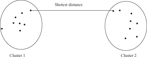
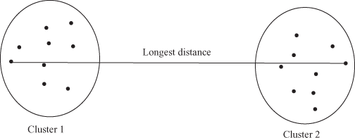

Figure 18.27 (a) Single linkage method, (b) Complete linkage method, (c) Average linkage method
The single linkage method also referred as the nearest neighbour approach is based on the principle of the shortest distance. The complete linkage method also referred as the farthest neighbour approach is based on the principle of the longest distance. In average linkage method, the distance between two clusters is defined in terms of the average of the distance between all the pairs of the subjects, in which one subject of the pair is from each of the clusters.
The second type of agglomerative method is the variance method. This method is mainly based on the concept of minimizing within the cluster variance. The most common and widely applied variance method is the ward’s method. In ward’s method, the distance is measured as the total sum of squared deviation from the mean of the concerned cluster to which the subject is allocated. In other words, for each subject, the squared Euclidean distance to cluster means is computed and then these computed distances are summed up for all the subjects. The formation of new clusters tends to increase the total sum of the squared deviations (error sum of squares). At each stage, two clusters are joined to produce the smallest increase in the overall sum of the squared within the cluster distances [Figure 18.28(a)]. The third type of agglomerative method is the centroid method. A cluster centroid is a vector containing one number for each variable, in which each number is the mean of the variable for the observations in that cluster. In this method, the distance between the two clusters is measured as the distance between their centroid. The two clusters are combined on the basis of the shortest distance between their centroids [Figure 18.28(b)].
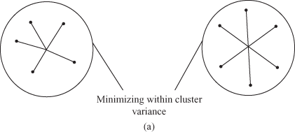
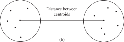
Figure 18.28 (a) Ward’s method, (b) Centroid method
The second type of agglomerative method is the variance method. This method is mainly based on the concept of minimizing within the cluster variance. The most common and widely applied variance method is the ward’s method.
The third type of agglomerative method is the centroid method. A cluster centroid is a vector containing one number for each variable, where each number is the mean of the variable for the observations in that cluster.
The second type of clustering method is the non-hierarchical clustering method that is also referred as k-means cluster analysis or iterative partitioning. As clear from Figure 18.26, this method can be classified into three categories: sequential threshold, parallel threshold, and optimizing partitioning.
The second type of clustering method is the non-hierarchical clustering method that is also referred as k-means cluster analysis or iterative partitioning.
In the sequential threshold non-hierarchical clustering method, first a cluster centre is selected and all the subjects within a pre-specified threshold value are grouped together. Next, a new cluster centre is selected, and the process is repeated for the unclustered subjects. It is important to note that once a subject is selected as a member of a cluster or as an associate of a cluster centre, it is not considered for clustering with the subsequent cluster centre or it is removed from further processing. The mode of operation in the parallel threshold method is the same except one difference in terms of the selection of several cluster centres simultaneously and then the subjects within a threshold level are clubbed to the nearest cluster centre. Then, this threshold level can be adjusted to accommodate some more subjects to the concerned cluster. In the optimizing threshold method, the subjects once assigned to a cluster can later be reassigned to another cluster to optimize an overall criterion measure such as the average within the cluster distance.
In the sequential threshold non-hierarchical clustering method, first a cluster centre is selected and all the subjects within a pre-specified threshold value are grouped together.
The mode of operation in the parallel threshold method is the same except one difference in terms of the selection of several cluster centres simultaneously and then the subjects within a threshold level are clubbed to the nearest cluster centre. Then, this threshold level can be adjusted to accommodate some more subject to the concerned cluster. In the optimizing threshold method, the subjects once assigned to a cluster can later be reassigned to another cluster to optimize an overall criterion measure such as the average within the cluster distance.
The non-hierarchical clustering method suffers from two major drawbacks. First, one has to pre-specify the number of clusters, and second, the cluster centre selection is arbitrary. This method is recommended when the number of observations is large. It has been recommended to first obtain the initial clustering solution by applying the hierarchical methods (may be ward’s). Next, the number of clusters or cluster centroids can be used as an input material to the optimizing partitioning method. Figures 18.29(a)–18.29(f) present the SPSS output for the problem already defined in the problem formulation stage. To understand the concept of the cluster analysis completely, it is important to understand the interpretation of Figures 18.29(a)–18.29(f).
The non-hierarchical clustering method suffers from two major drawbacks. First, one has to pre-specify the number of clusters, and second, the cluster centre selection is arbitrary.
Figure 18.29(a) is the simple statement of the number of cases, missing cases, and total number of cases. Figure 18.29(b) presents the Proximity matrix and is the matrix of proximity between subjects. The values in the table represent dissimilarities between each pair of items. The distance measure used in Figure 18.29(b) is the measure of dissimilarities (squared Euclidean distance). In the case of dissimilarities, the larger values indicate items that are very different. This figure gives some initial clues about clustering of subjects.


Figure 18.29 (a) Case processing summary, (b) Proximity matrix
Figure 18.29(c) presents the agglomeration schedule. This figure gives the information of how subjects are being clustered at each stage of the cluster analysis. The cluster analysis starts with 24 clusters at Stage 1, where Case 11 and Case 17 are combined (being minimum squared Euclidean distance). The coefficient column in Figure 18.29(c) indicates the squared Euclidean distance between the two clusters (or subjects) joined at each stage. After “coefficient column” “stage cluster first appears column” is shown. When we started the analysis, single cases existed, so it is indicated by zero at the initial stage. The last column “Next stage” indicates the subsequent stage at which the case combined in this cluster will be combined to another case. In the first row of this Column ‘2’ can be seen. Its interpretation can be done in Stage 2, where Case 7 is clustered with Case 11. Remember that Case 11 has already been clustered with Case 17 in Stage 1. On the basis of the squared Euclidean distance, this process continues until all the cases are clustered in a single group.

Figure 18.29 (c) Agglomeration schedule

Figure 18.29 (d) Cluster membership
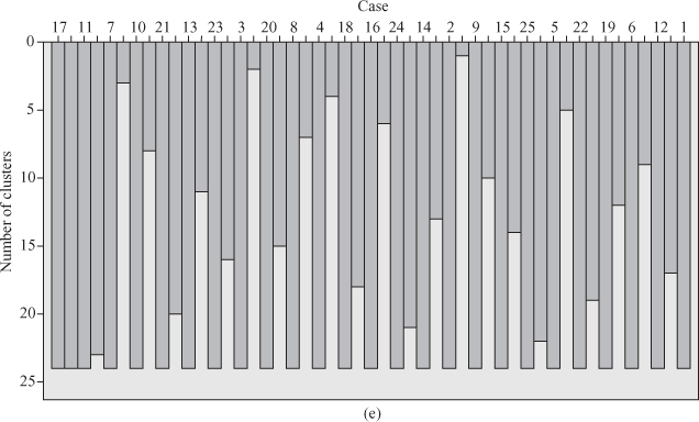
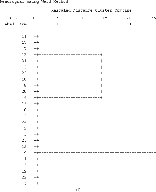
Figure 18.29 (e) Vertical icicle plot, (f) Dendrogram
Agglomeration schedule table gives the information of how subjects are being clustered at each stage of the cluster analysis.
The process described in the earlier paragraph can be well explained with the help of three examples in terms of clustering of Case 11 and Case 17 at Stage 1, Case 5 and Case 15 at Stage 11, and Case 3 and Case 13 at Stage 14, and Case 1 and Case 5 at Stage 20.
Cases 11 and 17 are grouped at Stage 1 with minimum squared Euclidean distance. These cases are not clustered before (see two zeros in “stage cluster first appears” below Clusters 1 and 2). In the “Next stage” column, Stage 2 is mentioned. This shows that Case 11 that was grouped with Case 17 in the first stage is grouped again with Case 7, making it a three-case cluster (Case 11, Case 17, and Case 7). This situation is shown in Figure 18.30.
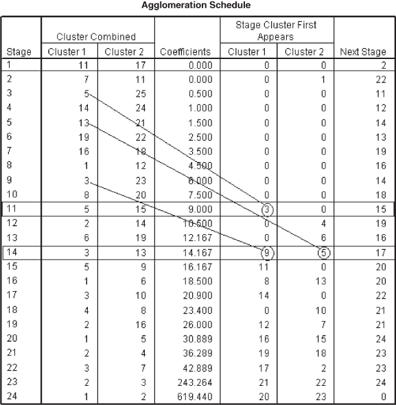
Figure 18.30 Joining of the cases or clusters at different stages
Cases 5 and 15 are grouped at Stage 11. In the “stage cluster first appears,” 3 and 0 are mentioned. It means that before clustering at this stage (Stage 11), cluster or Case 5 is first clubbed with Case 25 at Stage 3. Against Stage 11 in the “Next stage” column, Stage 15 is mentioned. This means at Stage 15, Case 5 will be grouped with Case 9 making it a three-case cluster (Case 5, Case 15, and Case 9). This situation is also shown in Figure 18.30.
At Stage 14, in the case of grouping of Case 3 and Case 13, it can be seen from Figure 18.30 that in the column “stages cluster first appears,” 9 and 5 are mentioned. It means that before clustering at this stage (Stage 14), cluster or Case 3 is first clubbed with Case 23 at Stage 9. Similarly, before clustering at this stage (Stage 14), cluster or Case 13 is first grouped with Case 21 at Stage 5. Thus, at Stage 14 there is a four-case cluster (Case 3, Case 13, Case 21, and Case 23). Against Stage 14 in the “Next stage” column Stage 17 is mentioned. This means at Stage 17, Case 3 will be grouped with Case 10 making it a five-case cluster. Interpretation of the other parts of the agglomeration schedule can be done on the same lines.
Figure 18.29(d) indicates ‘Cluster membership’ for each case. The SPSS has presented “two- to five-cluster” solutions as requested (is described in using the SPSS for Cluster analysis section). For example, if we take a three-cluster solution, Cases 1, 5, 6, 9, 12, 15, 19, 22, and 25 are the members of ‘Cluster 1.’ Cases 2, 4, 8, 14, 16, 18, 20, and 24 are the members of ‘Cluster 2.’ Cases 3, 7, 10, 11, 13, 17, 21, and 23 are the members of ‘Cluster 3.’ Similar interpretation can be done for other cluster solutions as well.
Figure 18.29(e) exhibits ‘Vertical icicle plot’ that displays some important information graphically. In fact, this plot generates the same information as generated by agglomeration schedule except that the values of distant measures are not shown in this plot. As can be seen from the first column of Figure 18.29(e), rows indicates “number of clusters.” Most importantly, this plot is interpreted from ‘bottom to top.’ In this problem, there are 25 subjects, and in the beginning, each subject is considered as individual cluster, so there are 25 initial clusters. At the first stage, two nearest subjects are combined (here these objects are Case 11 and Case 17) that results in 24 clusters. The bottom line of Figure 18.29(e) indicates that 24 clusters (as the plot is interpreted from “bottom to top”). As can also be seen from the agglomeration schedule, in the second stage two subjects Cases 7 and 11 are combined. Figure 18.29(e) shows that the column between 7 and 11 is of maximum length after the column between 11 and 17. In the next stage, Cases 5 and 25 are combined. See Figure 18.29(e), column between 5 and 25 is the third in length (from bottom to top) after “7 and 11” and “11 and 17”. In a similar manner, interpretation of other stages can be obtained.
Vertical icicle plot that displays some important information graphically.
Figure 18.29(f) is another graphical display as an output part of cluster analysis from the SPSS. This graphical plot is referred to as “dendrogram.” This tree diagram is a critical component of hierarchical clustering output.12 The dendrogram exhibits a relative similarity between subjects considered for cluster analysis. Dendrogram is interpreted from “left to right” in the form of “branches” that merge together as can be seen from Figure 18.29(f). On the upper part of the plot, one can see “Rescaled Distance Cluster Combine.” This indicates that cluster distances are rescaled to get the range of the output from “0 to 25” with 0 representing no distance and 25 representing the highest distance. Cases or clusters that are joined by nearest vertical line (from the left) are very similar, and cases or clusters that are joined by relative distant vertical line (from the left) are very dissimilar (Figure 18.31).
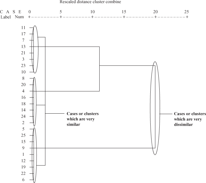
Figure 18.31 Joining of cases or clusters in a rescaled cluster distance
The “dendrogram” exhibits a relative similarity between subjects considered for cluster analysis.
- 18.2.4.4 A Decision Regarding Number of Clusters to be Retained in the Final Solution
A very important question in the cluster analysis is to determine the number of clusters. Virtually all clustering procedures provide little if any information as to the number of clusters present in the data.13 In fact, there is no strict rule to adhere to determine the number of clusters in cluster analysis. There are few guidelines that can be followed when determining the number of clusters. A brief discussion of these guidelines is given below:
In fact, there is no strict rule to adhere, to determine the number of clusters in cluster analysis.
- On the basis of theoretical considerations or experience of an executive, number of clusters can be prespecified.
- Agglomeration schedule and dendrogram can also be used to determine the required number of clusters in cluster analysis in terms of the distance measurement at which the clusters are combined. While reading agglomeration schedule, in a good cluster solution, a sudden jump appears. The stage just before the sudden jump point indicates the stopping point for merging of clusters. In the example taken for this chapter, at Stage 22 a sudden jump can be seen. So, this is a stopping point, and three-cluster solution will be a good solution in our case (Figure 18.32).

Figure 18.32 Determining number of clusters through agglomeration schedule
Dendrogram can also be used to determine the number of clusters in cluster analysis. Drawing an imaginary vertical line through dendrogram will present different cluster solutions. The first line in Figure 18.33 presents a three-cluster solution, one for each cut point where the branch of the dendrogram intersects the imaginary drawn vertical line. By considering different cut points, different number of cluster solutions can be obtained (as can be seen that second vertical line presents a two-cluster solution). A good cluster solution can be obtained by considering small within-cluster distances and large between-cluster distances. By tracing backward down the branches, cluster membership can be obtained.
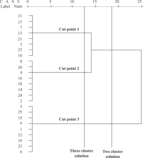
Figure 18.33 Determining number of clusters through dendrogram
Dendrogram can also be used to determine number of clusters in cluster analysis. Drawing an imaginary vertical line through the dendrogram will present different cluster solutions.
Number of clusters can also be determined by simply considering relative cluster size. From Figure 18.29(d) if we take simple frequency count of the cluster membership, then the number of clusters can be determined. Table 18.4 presents different number of cluster solutions with the number of subjects in the concerned cluster.
Table 18.4 Different number of cluster solutions with number of subjects in the concerned cluster
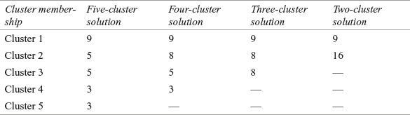
Number of clusters can also be determined by simply considering relative cluster size.
So, it can be seen from the table that a three-cluster solution presents a meaningful cluster solution with relative equal distribution of the subjects in concerned clusters.
18.2.4.5 Substantive Interpretation
After clustering, it is important to find the meaning of the concerned clusters in terms of finding some natural or compelling structure in the data. For this purpose, cluster centroid can be a useful tool. Remember that cluster centroid can be obtained through discriminant analysis. Figure 18.34 exhibits these cluster centroids. From the figure, it can be seen that Cluster 1 is associated with high values on Variables X1 (I am trying very hard to understand the loan schemes offered by different banks to purchase the product when it will be coming in the market), X3 (my old bike is old fashioned; I want to get rid of it), and X5 (I will not wait for product’s performance in the market, I know company is reputed and will certainly launch quality product). This cluster (Cluster 1) can be named as ‘desperate consumers.’ Cases 1, 5, 6, 9, 12, 15, 19, 22, and 25 are the members of ‘Cluster 1’ [see Figure 18.29(d)]. Cluster 2 has relatively low values on Variables X1, X3, and X5 and relative high value on Variable X6. Variable X6 is “companies always claim high about its product, let the product come in the market then only I will be taking any decision about the purchase.” This cluster (Cluster 2) can be named as ‘patient consumers.’ Cases 2, 4, 8, 14, 16, 18, 20, and 24 are the members of ‘Cluster 2’ [see Figure 18.29(d)]. Cluster 3 has relative high values on Variables X2 (I am still in confusion whether to sell my old bike), X4 (my company has promised that it will be releasing a much awaited new incentive scheme; purchase of new model is based on this factor), and X7 (I want to purchase a new bike but my kids are growing up and are demanding to purchase a car instead of bike, which I already have). This cluster (Cluster 3) can be named ‘perplexed consumers.’ Cases 3, 7, 10, 11, 13, 17, 21, and 23 are the members of ‘Cluster 3’ [see Figure 18.29(d)].
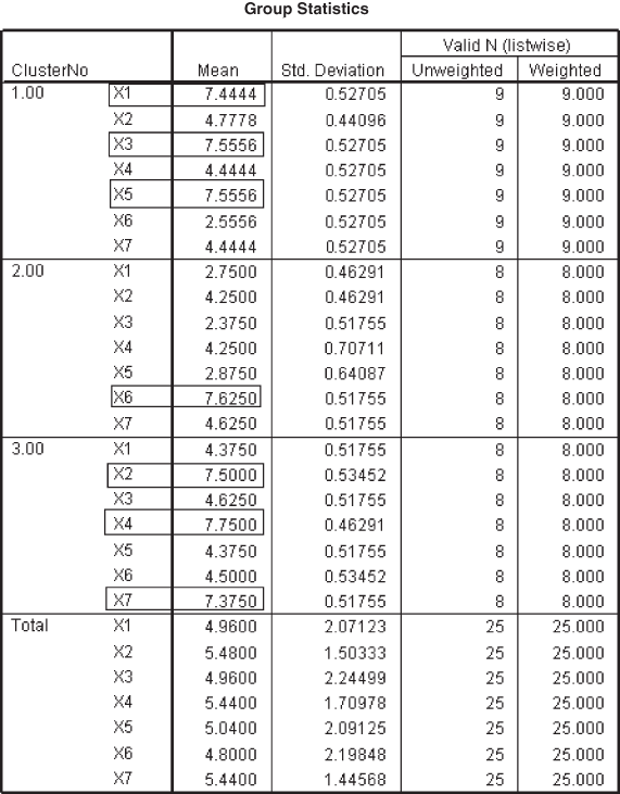
Figure 18.34 Cluster centroids obtained through discriminant analysis
18.2.4.6 Check the Model Fit
Formal procedures for testing statistical reliability of clusters are not fully defensible. Following are some ad hoc procedures to put a rough check on the quality of cluster analysis.
- Perform the cluster analysis on same data using different distance measures and compare the results across distance measures. In addition, different methods of clustering for the same data can be used and the result can be compared.
- Split the data into halves and perform the cluster analysis on the halves. Obtained cluster centroid can be compared across subsamples.
- Delete various variables from the original sets of variables and perform the cluster analysis on remaining set of variables. Obtained result should be compared with the result obtained from the original set of variables.
18.2.5 Non-Hierarchical Clustering
As discussed earlier, to get the optimum cluster solution, hierarchical clustering procedure must be used first to obtain the number of clusters and then these number of clusters can be used as the basis of initial information to perform k-means cluster analysis (non-hierarchical clustering procedure). The k-means cluster analysis typically involves minimizing the within-cluster variation or, equivalently, maximizing the between-cluster variation.14 In the hierarchical clustering method, a three-cluster solution is obtained for the motorbike company example discussed in the beginning of this section. Using this information, the SPPS output for the problem at the beginning of this section through k-means cluster analysis (non-hierarchical clustering procedure) is presented in the form of Figure 18.35(a) to 18.35(g).
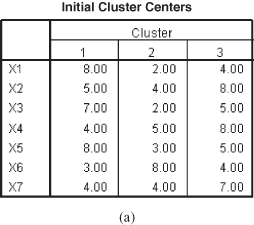
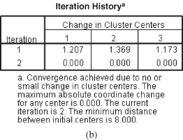
Figure 18.35 (a) Initial cluster centers, (b) Iteration history
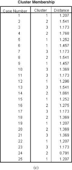

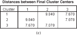

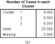
Figure 18.35 (c) Cluster membership, (d) Final cluster centers, (e) Distance between final cluster centers, (f) ANOVA table, (g) Number of cases in each cluster
First, the hierarchical clustering procedure must be used to obtain the number of clusters and then these numbers of clusters can be used as the basis of initial information to perform the k-means cluster analysis (non-hierarchical clustering procedure).
Figure 18.35(a) exhibits Initial cluster centers. These initial cluster centers are the values of three randomly selected cases. The SPSS by default selects the cases that are dissimilar and then cases join these initial values (based on similarity) to make distinct clusters. Each subject joins nearest classification cluster center and the process continues until the stopping criteria is reached.
Figure 18.35(b) presents Iteration history and is the progress of estimation process for each iteration. In each iteration, cases join different clusters, as a result cluster center changes. Any number in the second row of Figure 18.35(b) against “iteration 2” indicates the distance of new cluster center (after joining of cases) from the previous cluster center. When a zero appears in the rows against iteration, change in distance is very small, and stopping criteria is achieved to obtain final solution.
Figure 18.35(c) presents Cluster membership. As the name indicates, this figure shows the cluster membership information for each case. In the “Distance” column, distance between the subject and cluster center is given. This distance can be used to obtain some knowledge about the “representativeness” of the case for the concerned cluster. A small distance indicates that the cases are good representative of the cluster and a large distance indicates the cases are not good representative of the cluster.
Figure 18.35(d) shows ‘Final cluster centers’. Values in the figure indicate means for each variable within each final cluster. It can be seen that first cluster has high cluster-center values on Variables X1, X3, and X5. This cluster has also a relatively low value for Variable X6. Second cluster has relatively high cluster-center value for Variable X6. Third cluster has relatively high cluster-center value on Variables X2, X4, and X7.
Figure 18.35(e) shows Distance between final cluster centers and the “Euclidean Distances” between the final cluster centers. Relatively large values indicate that clusters are different from each other. However, relatively small values indicate that clusters are not so different from each other.
Figure 18.35(f) exhibits ANOVA table. This figure indicates the variables that are most important in cluster solution and cluster analysis. Mean square in the Cluster column indicates the variance in the variable that can be attributed to clusters. Mean square in the Error column indicates the variance in the variable that cannot be attributed to clusters. F ratio indicates the ratio of cluster variance to error variance. Large F value indicates variables that are important for segregating the clusters. Small F value (close to 1) indicates variables that are not very useful in identifying the membership of the clusters. F statistic should not be interpreted in the traditional way and hence the significance value associated with F value cannot be interpreted in the traditional manner, in terms of acceptance or rejection of null hypothesis.
Large F value indicates variables that are important for segregating the clusters. Small F value (close to 1) indicates variables that are not very useful in identifying the membership of cluster.
F statistic should not be interpreted in the traditional way and hence the significance value associated with F value cannot be interpreted in the traditional manner, in terms of acceptance or rejection of null hypothesis.
Figure 18.35(g) presents Number of cases in each cluster. This figure shows number of cases assigned to each cluster. A big mismatch in the proportional size of the cluster is an indication of some problem in the cluster solution. For example, if Cluster 1 has got 18 members and Clusters 2 and 3 have only 3 and 4 members, respectively, then there is some problem with the cluster solution. In this kind of situation, the number of clusters requested should be rechecked, and included list of variables in the cluster analysis must be re-examined in light of its importance in the cluster analysis.
18.2.6 Using the SPSS for Hierarchical Cluster Analysis
In case of using the SPSS for conducting cluster analysis, first click Analyze/Classify/Hierarchical Cluster. Hierarchical Cluster Analysis dialogue box will appear on the screen (Figure 18.36). In this dialogue box, first select all the seven variables taken for the study and place it in the ‘Variables’ box. From ‘Cluster’ select ‘Cases’ and from ‘Display’ select ‘Statistics’ and ‘Plots.’ As a next step, click ‘Statistics,’ given in the right upper part of the Hierarchical Cluster Analysis dialogue box (Figure 18.36). Hierarchical Cluster Analysis: Statistics dialogue box will appear on the screen. In this dialogue box, select ‘Agglomeration schedule’ and ‘Proximity matrix.’ From ‘Cluster Membership’ select ‘Range of solutions.’ Against ‘Minimum number of clusters’ place ‘2’ and against ‘Maximum number of clusters’ place ‘5’ (Figure 18.37). It has already been discussed that a researcher can select number of clusters on the basis of different ground or his discretion. Click Continue. Hierarchical Cluster Analysis dialogue box will reappear on the screen. From this dialogue box, click ‘Plots.’ Hierarchical Cluster Analysis: Plots dialogue box will appear on the screen. In this dialogue box, select ‘Dendrogram,’ from ‘Icicle’ select ‘All clusters,’ from ‘Orientation’ select ‘Vertical’ and click Continue (Figure 18.38). Hierarchical Cluster Analysis: Plots dialogue box will reappear on the screen. In this dialogue box, click ‘Method.’ Hierarchical Cluster Analysis: Method dialogue box will appear on the screen. From ‘Cluster Method’ select ‘Ward’s method,’ and from ‘Measure’ select ‘Interval’ and then select ‘Squared Euclidean distance’ (Figure 18.39). Click Continue. Hierarchical Cluster Analysis dialogue box will reappear on the screen. In this dialogue box, click Save. Hierarchical Cluster Analysis: Save dialogue box will appear on the screen (Figure 18.40). In this dialogue box, if “Range of solutions” are selected and if against minimum number of clusters and maximum number of clusters “2 and 5” are placed then the SPSS will print “cluster membership” in the data sheet also (Figure 18.40). Click Continue. Hierarchical Cluster Analysis dialogue box will reappear on the screen. Click OK. The SPSS output as exhibited in Figures 18.35(a) to 18.35(g) will appear on the screen.
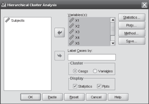
Figure 18.36 SPSS Hierarchical Cluster Analysis dialogue box
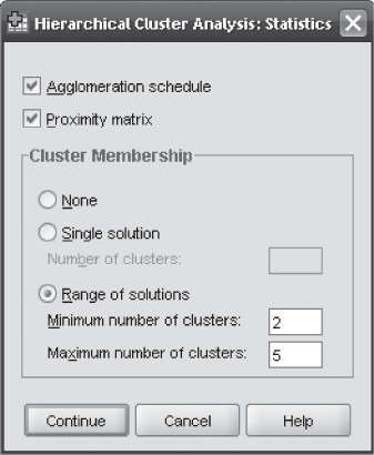
Figure 18.37 SPSS Hierarchical Cluster Analysis: Statistics dialogue box

Figure 18.38 SPSS Hierarchical Cluster Analysis: Plots dialogue box

Figure 18.39 SPSS Hierarchical Cluster Analysis: Method dialogue box

Figure 18.40 SPSS Hierarchical Cluster Analysis: Save dialogue box
18.2.7 Using the SPSS for Non-Hierarchical Cluster Analysis
In case of using the SPSS for conducting non-hierarchical cluster analysis, first click Analyze → Classify → k-Means Cluster. The k-Means Cluster Analysis dialogue box will appear on the screen (Figure 18.41). In this dialogue box, first select all the seven variables taken for the study and place it in the ‘Variables’ box. In the hierarchical clustering method, we have already found out that the required number of clusters are three. In k-Means Cluster Analysis dialogue box, place ‘3’ in the ‘Number of Clusters’ box. From ‘Method’ select ‘Iterate and classify’ and click Iterate given at the upper right in the k-Means Cluster Analysis dialogue box. The k-Means Cluster Analysis: Iterate dialogue box will appear on the screen (Figure 18.42). In this dialogue box, place ‘2’ against ‘Maximum Iterations’ and place ‘0’ against ‘Convergence Criterion.’ It is important to note that in the SPSS, by default, maximum iterations are 10. Here, if we had placed “10” (as by default) instead of “2” then we would have got the same solution as exhibited in Figure 18.35 because convergence criterion 0 has already been achieved in the second iteration. For complex problems, by default the SPSS iteration 10 can be increased to obtain the convergence criterion 0. Click Continue. The k-Means Cluster Analysis dialogue box will reappear on the screen. From this dialogue box, click Save. K-Means Cluster Analysis: Save dialogue box will appear on the screen (Figure 18.43). In this dialogue box, select ‘Cluster membership’ and ‘Distance from cluster centre’ and click Continue. The k-Means Cluster Analysis dialogue box will reappear on the screen. From this dialogue box, Click ‘Options.’ The k-Means Cluster Analysis: Options dialogue box will appear on the screen (Figure 18.44). In this dialogue box, from ‘Statistics’ select ‘Initial cluster centres,’ ‘ANOVA table,’ and ‘Cluster information for each case.’ Click Continue. The k-Means Cluster Analysis dialogue box will reappear on the screen. In this dialogue box, Click OK, the SPSS output as exhibited in Figures 18.35(a) to 18.35(g) will appear on the screen.
Endnotes |
1. Raven, M. R. (1990). “The Application of Exploratory Factor Analysis in Agriculture Education Research”, Journal of Agriculture Education, 35(4): 9–14.
2. Hair, J. F., W. C. Black, B. J. Babin, R. E. Anderson and R. L. Tatham (2009). Multivariate Data Analysis, 6th ed., p. 125. Pearson Education.
3. Aaker, D. A., V. Kumar and G. S. Day (2000). Marketing Research, 7th ed., p. 554. Wiley.
4. Fabrigar, L. R., D. T. Wegener, R. C. MacCallum and E. J. Strahan (1999). “Evaluating the Use of Exploratory Factor Analysis in Psychological Research”, Psychological Methods, 4(3): 272–99.
5. Cattell, R. B. (1966). “The Screen Test for the Number of Factors”, Multivariate Behavioural Research, 1(2): 245–76.
6. Bentler, P. M. and K. H. Yuan (1998). “Tests for Linear Trend in the Smallest Eigenvalues of the Correlation Matrix”, Psychometrica, 63(2): 131–44.
7. Reise, S. P., N. G. Waller and A. L. Comrey (2000). “Factor Analysis and Scale Revision”, Psychological Assesment, 12(3): 287–97.
8. Fabriger, op. cit., p. 650.
9. Costello, A. B. and J. W. Osborne (2005). “Best Practices in Exploratory Factor Analysis: Four Recommendations for Getting the Most from Your Analysis”, Practical Assessment, Research & Evaluation, 10(7): 1–9.
10. Punj, G. and D. W. Stewart (1983). “Cluster Analysis in Marketing Research: Review and Suggestions for Applications”, Journal of Marketing Research, 20: 134–48.
11. Zikmund, W. G. (2007). Business Research Methods, 7th ed., p. 589. South-Western Thomson Learning.
12. Lehmann, D. R., S. Gupta and J. H. Steckel (1998). Marketing Research, p. 575. Addison-Wesley.
13. Milligan, G. W. and M. C. Cooper (1985). “An Examination of Procedures for Determining the Number of Clusters in a Data Set”, Psychometrica, 50(2): 159–79.
14. Magidson, J. and J. K. Vermunt (2002). “Latent Class Models for Clustering: A Comparison with K-Means”, Canadian Journal of Marketing Research, 20: 37–44.
Summary |
The techniques described in this chapter, namely, factor analysis and cluster analysis are often referred to as “interdependence analysis.” Factor analysis is a very useful technique of data reduction and summarization. The main focus of factor analysis is to summarize the information contained in a large number of variables into few small numbers of factors. Factor analysis is performed using the following steps: problem formulation, construction and examination of correlation matrix, selection of an appropriate factoring technique, a decision regarding the number of factors to be retained in the final solution, factor rotation for enhancing the interpretability of the solution, substantive interpretation, and check the model fit.
Cluster analysis is a technique of grouping individuals or objects or cases into relatively homogeneous (similar) groups. These homogeneous groups are often referred to as clusters. The subjects grouped within the cluster are similar to each other, and there is dissimilarity between the clusters. Cluster analysis is performed using six steps. These six steps are as follows: problem formulation, choice of an appropriate proximity or similarity measure, selection of an appropriate clustering technique, a decision regarding the number of clusters to be retained in the final solution, substantive interpretation, and check the model fit. To get the optimum cluster solution, first hierarchical clustering procedure must be used to obtain the number of clusters and then this number of clusters can be used as the basis of initial information to perform k-means cluster analysis (non-hierarchical clustering procedure).
Key Terms |
% of variance, 660
Agglomeration schedule, 681
ANOVA table, 691
Average linkage method, 678
Bartlett’s test of sphericity, 654
Centroid method, 679
Cluster analysis, 674
Cluster membership, 674
Communality, 654
Complete linkage method, 678
Correlation matrix, 654
Dendrogram, 674
Distance between final cluster centers, 691
Euclidean distance, 676
Eigenvalue, 654
Factor loading plot, 655
Factor loadings, 654
Factor matrix, 654
Factor score, 655
Factors, 660
Final cluster center, 691
Hierarchical clustering approach, 677
Icicle plot, 674
Initial cluster centres, 689
Interdependence analysis, 652
Iteration history, 690
Kaiser-Mayer-Olkin measure of sampling adequacy, 654
Linkage method, 678
Non-hierarchical clustering approach, 679
Number of cases in each cluster, 691
Oblique rotation, 664
Orthogonal rotation, 664
Parallel threshold optimizing partitioning, 679
Principal axis factoring, 660
Rotation, 663
Scree plot, 654
Sequential threshold, 679
Single linkage method, 664
Sudden jump, 678
The principal component method, 660
Variance method, 679
Variance methods and centroid method, 679
Varimax procedure, 664
Ward’s method, 679
Notes |
- 1. www.indiastat.com, accessed September 2009, reprinted with permission.
- 2. http://www.bata.in/page.php?kon=5_2_1, accessed October 2009.
- 3. http://www.telegraphindia.com/1060331/asp/others/print.html.
Discussion Questions |
- 1. What is the conceptual framework of factor analysis? Under what circumstances a researcher should apply factor analysis.
- 2. What are the steps used in performing factor analysis?
- 3. Write short note on following topics related to factor analysis:
(a) Estimation or analysis sample
(b) Communality
(c) Correlation matrix
(d) Kaiser-Mayer-Olkin measure of sampling adequacy
(e) Bartlett’s test of sphericity
(f) Eigenvalue, % of variance
(g) Scree plot, factor loadings
(h) Factor matrix and factor score
(i) Factor loading plot
(j) The principal component method
(k) Principal axis factoring
(l) Varimax procedure
(m) Orthogonal rotation
(n) Oblique rotation
- 4. What is the conceptual framework of cluster analysis? Under what circumstances a researcher should apply cluster analysis.
- 5. What are the steps used in performing cluster analysis?
- 6. Explain the difference between hierarchical clustering technique and non-hierarchical clustering technique. What is the use and application of clustering technique in making managerial decisions.
- 7. Write short note on following topics related to cluster analysis:
(a) Agglomeration schedule
(b) Cluster membership
(c) Icicle plot
(d) Dendrogram
(e) Euclidean distance
(f) Linkage method
(g) Variance methods and centroid method
(h) Single linkage method
(i) Complete linkage method
(j) Average linkage method
(k) Variance method
(l) Ward’s method
(m) Centroid method
(n) Dissimilarity matrix
(o) Cluster membership
(p) Final cluster centre
(q) Distance between final cluster centres
(r) ANOVA table in clustering
Case Study |
Case 18: Britannia Industries Ltd: A leading player in Indian Bakery Industry
Introduction: An Overview of Indian Bakery Industry
Indian bakery industry is mainly dominated by small-scale sector. In India, bakery products primarily include biscuits and bread. The two major bakery products in India are biscuits and bread that accounts for 82% of all bakery production. For all the leading companies producing bakery products, biscuits have got the lion’s share in total sales. In the year 2001–2002, demand for biscuits was 1188 thousand metric tonnes, which is estimated to increase to 2758 thousand metric tonnes in the year 2014–2015. Market segmentation wise organized and unorganized market secure 50% of the total market size. In the time span of 2009–2010 to 2014–2015, the market is estimated to grow at a rate of 6.2%. Biscuit market is also segmented with respect to product line. Glucose, Milk, Marie, Cream, Crackers, and others occupy 60%, 10%, 10%, 5%, 7%, and 8% of the total market, respectively. Britannia and Parle are two major players in the biscuit market. In the year 2001–2002, demand for bread was 12.85 billion rupees, which is estimated to increase to 26.90 billion rupees in the year 2014–2015. For bread, only 15% market is occupied by the organized players and 85% market is captured by unorganized players. In the time span of 2009–2010 to 2014–2015, bread market is estimated to grow at a rate of 5.0%. Milk bread has got the lion’s share with 85% of share of the total market. Modern food and Britannia are two major producers of bread.1
Britannia Industries Limited: A Leading Player in Indian Bakery Industry
Britannia Industries Ltd is a leading bakery products company in India with a predominant focus on the sale of branded biscuits. The company’s history goes back to 1892, when it was incorporated in Kolkata under the name of Britannia Biscuit Company. BIL got its current name in 1979. In 1993, the Nusli Wadia group acquired a stake in BIL’s parent company, Associated Biscuits International Ltd, UK and became an equal partner in BIL with the French Major Groupe Danone. The company is engaged in the business of biscuits, bread, cakes, and rusks. It caters to diverse needs and tastes of the Indian consumer across age groups through its optimum range of biscuit brands. Some of its popular brands are Tiger, Good Day, Marigold, Milk Bikis, Treat, 50:50, Little Heart, Bourbon, Pure Magic, Snax, Premium Bake, and Nutrichoice. The company’s strategy of consistently renovating its existing brands and launching new ones has helped it to garner larger share of the Indian biscuits market every year. In the year 2005–2006, the company’s market share stood at 37.2%. Britannia is the pioneer in the sliced bread business in India. Today, it caters to almost half the branded bread market in India. Its cake and rusk business, albeit small, has been growing at a healthy pace. However, the bread, cakes, and rusk business together accounts for only 8.9% of the company’s total turnover. It is essentially a biscuit company with 90.2% revenue coming from the sale of biscuits.2
The company has also been following the inorganic route of expansion quite actively in the recent past. It made its first international acquisition in March 2007 by buying 70% stake in Strategic Food International Co LLC, Dubai, a leading company in the biscuits and cookies segment in the GCC (Gulf Cooperation Council) markets. In July 2005, it acquired 50% stake in Bangalore-based Daily Bread. The company believes that this acquisition will help increase its presence in select markets with a range of gourmet sold under the brand names Daily Bread and Deluca. In addition to the bakery business, Britannia runs its dairy operations through its joint venture Britannia New Zealand Foods Pvt. Ltd. This joint venture with Fonterra of New Zealand was formed in 2002 by demerging the dairy products business from the Britannia Industries Limited.2 Table 18.01 below exhibits sales and profit after tax (in million rupees) of the Britannia Industries Limited from 1994–1995 to 2007–2008. The company has registered encouraging profit after tax figure in the financial year 2007–2008.
TABLE 18.01 Sales and profit after tax (in million rupees) of Britannia Industries Limited from 1994–1995 to 2007–2008
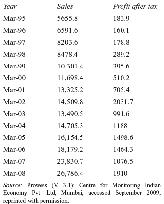
Britannia Plans to Consolidate Factories, Realign Operations
Britannia’s non-biscuit business like breads, rusks, cakes, and dairy business is gaining in size. In the light of this development, biscuit giant Britannia is working on operational realignment aimed at streamlining the number of manufacturing locations as well as reworking its distribution strategy. Company’s Managing Director Ms Vinita Bali told The Economic Times, “Britannia’s bread, cake and rusk portfolio has quadrupled in the past four years with a run rate of about Rs 4000 million right now. We will consolidate factories across our bakery products and realign operations wherever it makes sense.” Ms Bali added about the realignment strategy of the Britannia Industries, “The realignment is being done to increase cost effectiveness, reduce complexity and to adopt a synergistic go-to-market strategy.” Britannia has also strategies to streamline its marketing play into four key paths, namely, modern trade, general trade, rural markets, and transit routes. In the line of this segment, Britannia has introduced smaller SKUs at more buoyant price points over the past 2–3 months. Company has plans to sale through confectionary selling points by offering small packets of biscuits. This is a strategy to shift from grocery segment to confectionary segment. Vice President and COO of Britannia Industries Mr Neeraj Chandra said, “By positioning it as a single serve offering, we have made the range more accessible. It will bring a larger section of the customer base into our ambit.”3
Suppose the Britannia Industries wants to introduce a very small packet of a famous brand of biscuits to stick to its policy of catering market through grocery stores. For this purpose, suppose the company wants to ascertain consumer perception about the policy of launching very small packets of biscuits. Take the help of literature to list down the statements that can be used to ascertain consumer perception. Use the techniques presented in the chapter to factorize (group) these statements into some variables. Use any software output to determine the required factors and discuss the result in the light of launching a research plan indicating required multivariate analysis to treat the independent variables and dependent variable (consumer perception).
Suppose the company wants to place few products as per the preference or taste of the consumers. Use literature to list down some attributes (statements) related to the taste of the customers for biscuits. These statements can be collected on some taste attributes like salty, light salty, spicy, sweet, light sweet, mix of sweet and salt, and so on. Collect data on these statements on a 7-point rating scale from randomly selected consumers. Apply the clustering techniques (using any statistical software) presented in this chapter to group individuals on common clustering attributes. Discuss the result to present a suitable strategy to the company on the basis of clustering of the consumers.
Notes |
- 1. www.indiastat.com, accessed September 2009, reprinted with permission.
- 2. Prowess (V. 3.1): Centre for Monitoring Indian Economy Pvt. Ltd, Mumbai, accessed September 2009, reprinted with permission.
- 3. http://economictimes.indiatimes.com/articleshow/ 4553714.cms?prtpage=1, accessed September 2009, reprinted with permission.