
Chapter 14
Non-Parametric Statistics
Learning Objectives
Upon completion of this chapter, you will be able to:
- Analyse nominal as well as ordinal level of data
- Learn relative advantages of non-parametric tests over parametric tests
- Understand when and how to use the runs test to test randomness
- Understand when and how to use the Mann–Whitney U test, the Wilcoxon matched-pairs signed rank test, the Kruskal–Wallis test, the Friedman test, and Spearman’s rank correlation
Statistics in Action: Bajaj Electricals ltd
Bajaj Electricals Ltd (BEL) is part of the Rs 200 billion Bajaj group, which is in the business of steel, sugar, two wheelers, and three wheelers besides an impressive range of consumer electrical products. BEL is a 70-year old company with a turnover of over Rs 14,040 million and aiming to be a Rs 20,010 million company in the next couple of years. The company operates across diverse sectors such as home appliances, fans, lightings, luminaries and engineering, and projects. It has also undertaken various engineering projects in the area of manufacturing and erection of transmission line towers, telecom towers, mobile, and wind energy towers.1
Bajaj has embarked on an ambitious journey “Action 2008” to achieve a sales turnover of Rs 20,010 million in the financial year 2009–2010 after emerging victorious in mission “Zoom Ahead” by becoming a Rs 14,040 million company in the financial year 2007–2008.2 Bajaj Electricals Ltd has its own unique work culture. Mr Shekher Bajaj in an article published in the Economic Times wrote “Every individual has the potential to perform if he or she gets proper motivation, the right opportunity, and freedom to work. In the long run, success is achieved when ordinary people perform extraordinarily. It is important to keep an open mind rather than drawing preconceived impression about people. More often that not, such impressions will be proven wrong.”3
Let as assume that a researcher wants to study the differences in the satisfaction levels of Bajaj dealers with respect to the company’s policies in Madhya Pradesh and Chhattisgarh. The satisfaction scores (taken from 7 dealers) from the two states are given in Table 14.1.
Table 14.1 Satisfaction scores of dealers

As discussed in previous chapters, the t-test to compare the means of two independent populations can be applied. Here, the researcher might be doubtful about the normality assumption of the population. Is there any way to analyse the data in this situation? Suppose the researcher wants to ascertain the difference in dealer satisfaction levels in four states: Madhya Pradesh, Chhattisgarh, Gujarat, and Maharashtra. The researcher has collected scores from 7 dealers of Gujarat and Maharashtra. One-way analysis of variance (ANOVA) technique can be applied for finding out the difference in mean scores. However the researcher is doubtful about the ANOVA assumptions of normality, independent groups, and equal population variance. Is there any way to analyse the data when assumptions of ANOVA are not met?
In most research processes, data are either nominal or ordinal. How can nominal and ordinal data be analysed. This chapter focuses on answers to such questions. It also discusses the runs test; the Mann–Whitney U test, the Wilcoxon matched-pairs signed rank test, the Kruskal–Wallis test, the Friedman test, and Spearman’s rank correlation.
14.1 Introduction
All the tests that we have discussed so far except the chi-square test are parametric tests. We will focus on some important non-parametric tests in this chapter. First, we need to understand the difference between parametric and non-parametric tests. Parametric tests are statistical techniques to test a hypothesis based on some restrictive assumptions about the population. Generally, these assumptions are with respect to the normality of the population and random selection of samples from the normal population. Additionally, parametric tests require quantitative measurement of the sample data in the form of an interval or ratio scale.
Parametric tests are statistical techniques to test a hypothesis based on some restrictive assumptions about the population. Generally, these assumptions are with respect to the normality of the population and random selection of samples from the normal population. Additionally, parametric tests require quantitative measurement of the sample data in the form of an interval or ratio scale.
When a researcher finds that the population is not normal or the data being measured is qualitative in nature, he cannot apply parametric tests for hypothesis testing and he has to use non-parametric tests. Non-parametric tests are not dependent upon the restrictive normality assumption of the population. Additionally, non-parametric tests can be applied to nominal and ordinal scaled data. These tests are also referred to as distribution free statistics (do not require the population to be normally distributed). The relative advantages of non-parametric tests over parametric tests are as follows:
Non-parametric tests are not dependent upon the restrictive normality assumption of the population. Additionally, non-parametric tests can be applied to nominal and ordinal scaled data. These tests are also referred to as distribution free statistics (do not require the population to be normally distributed).
- Non-parametric tests can be used to analyse nominal as well as ordinal level of data.
- When sample size is small, non-parametric tests are easy to compute.
- Non-parametric tests are not based on the restrictive normality assumption of the population or any other specific shape of the population.
However, non-parametric tests also possess some limitations. Some of the limitations of non-parametric tests are as follows:
- When all the assumptions of parametric tests are met, non-parametric tests should not be applied.
- When compared to parametric tests, availability and applicability of non-parametric tests are limited.
- When sample size is large, non-parametric tests are not easy to compute.
Though a large number of non-parametric tests are available, this chapter will focus only on a few widely used non-parametric tests. In general, the vast majority of non-parametric tests are rank-based tests.1 Specifically, we will discuss the following tests;
- Runs test
- Mann–Whitney U test
- Wilcoxon matched-pairs signed rank test
- Kruskal–Wallis test
- Friedman test
- Spearman’s rank correlation
14.2 Runs Test for Randomness of Data
All statistical tests are based on the randomness of samples drawn from the population. In some cases, researchers are apprehensive about the randomness of the sample when the sample exhibits orderly arrangement, which is rarely obtained by random sampling. The following example explains this concept clearly.
A company wants to send 20 employees (from the Finance and Marketing departments) for advanced training from a large population (all the employees of the company). The company’s administrative officer has selected the following samples randomly (where F represents selection from the Finance department and M represents selection from the Marketing department):
F,F,F,F,M,M,M,M,F,F,F,F,M,M,M,M,F,F,F,F
One can doubt the randomness of the sample just by inspection as it is rare to find such ordered arrangement in a random sample. We can test the randomness of the sample using the runs test. A run is defined as the sequence of identical occurrence of the elements (numbers or symbols), preceded or followed by different occurrence of the elements or by no elements at all. The number of observations in each run defines the length of a run.2 In the above example, there are five runs as shown below:
The randomness of the sample can be tested by using the runs test. A run is defined as the sequence of identical occurrence of the elements (numbers or symbols), preceded or followed by different occurrence of the elements or by no elements at all.
14.2.1 Small-Sample Runs Test
The small-sample runs test is an appropriate choice in cases where the sample size is small. The sample size is considered to be small when n1 and n2 are less than or equal to 20, where n1 is the number of occurrences of Type 1 and n2 is the number of occurrences of Type 2. When the sample size is small, the runs tests is carried out by comparing the observed number of runs, R, with the critical values of runs for given values of n1 and n2. The critical values of R for the lower tail and for the upper tail is given in the appendices. The null and alternative hypotheses can be stated as below:
In cases where the sample size is small, the small-sample runs test is an appropriate choice. The sample is considered to be small when n1 and n2 are less than or equal to 20, where n1 is the number of occurrences of Type 1 and n2 is the number of occurrences of Type 2.
H0: The observations in the sample are randomly generated.
H1: The observations in the sample are not randomly generated.
If the observed value of R falls in between the lower-tail critical value and the upper-tail critical value of R, the null hypothesis is accepted and the alternative hypothesis is rejected. To check the randomness of samples in the example stated above, we need to adopt the seven step procedure of hypothesis testing discussed previously. Example 14.1 explain how the hypothesis testing procedure can be used for the runs test.
Example 14.1
A company wants to send 20 employees selected randomly from the finance and marketing departments for advanced training. The company’s administrative officer has selected random samples as below:
F,F,F,F,M,M,M,M,F,F,F,F,M,M,M,M,F,F,F,F
Test the randomness of the sample.
SolutionThe seven steps of hypothesis testing can be performed as below:
Step 1: Set null and alternative hypotheses
H0: The observations in the samples are randomly generated.
H1: The observations in the samples are not randomly generated.
Step 2: Determine the appropriate statistical test
In this example, n1 is the number of occurrences of Type 1 that is, the number of occurrences from the Finance department and n2 is the number of occurrences of Type 2, that is, the number of occurrences from the Marketing department. So, n1 = 12 and n2 = 8. Both n1 and n2 are less than 20. Hence, the small-sample runs test is an appropriate choice.
Step 3: Set the level of significance
The confidence level is taken as 95% (a = 0.05) in this case.
Step 4: Set the decision rule
For n1 = 12 and n2 = 8, from the table (given in the appendices), the critical value of R for the lower tail is 6 and the critical value of R for the upper tail is 16. If runs are less than 6 and more than 16, the decision is to reject the null hypothesis and accept the alternative hypothesis.
Step 5: Collect the sample data
The sample data are given as
F,F,F,F,M,M,M,M,F,F,F,F,M,M,M,M,F,F,F,F
Step 6: Analyse the data
The number of runs are 5 as shown below:
Step 7: Arrive at a statistical conclusion and business implication
The number of runs 5 is less than the critical value of R for the lower tail, that is, 6. Hence, the decision is to reject the null hypothesis and accept the alternative hypothesis. So, it can be concluded that the observations in the sample are not randomly generated.
The company has to reconsider the sampling technique used to maintain the randomness of the sample. Figures 14.1 and 14.2 are the outputs for Example 14.1 produced using Minitab and SPSS, respectively.
14.2.2 Using Minitab for Small-Sample Runs Test
The first step is to click Stat/Nonparametrics/Runs Test. The Runs Test dialog box will appear on the screen (Figure 14.3). In the Variables box, numeric data should be entered. We need to code the data for this purpose. Finance is coded as 1 and Marketing is coded as 2. Place the coded data in the Variables box. From Figure 14.3, we can see that the test default is “Above and below the mean.” This means that the test will use the mean of the numbers to determine when the run stops. One can place a value by selecting the second circle. Click OK. Minitab will produce the output as shown in Figure 14.1. In the output, K, is the average of values, which is generally used as the divider of runs. From the output, the p value clearly indicates the rejection of the null hypothesis and the acceptance of the alternative hypothesis.
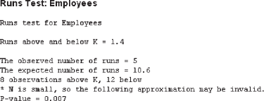
Figure 14.1 Minitab output for Example 14.1
14.2.3 Using SPSS for Small-Sample Runs Tests
The first step is to click Analyze/Nonparametric/Runs. The Runs Test dialog box will appear on the screen (Figure 14.4). Place employees in the Test Variable List box and select Mean as a Cut Point and click OK. The output shown in Figure 14.2 will appear on the screen. Note that the data coding procedure is exactly the same as discussed in the section on using Minitab for small-sample runs tests.
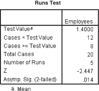
Figure 14.2 SPSS output for Example 14.1
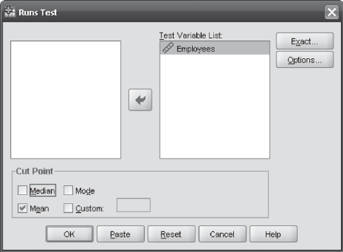
Figure 14.4 SPSS Runs Test dialog box
Note: MS Excel cannot be used directly for any of the non-parametric tests. It can only be used indirectly for simple computations that help in these tests.
14.2.4 Large-Sample Runs Test
For n1 and n2 greater than 20 (or either n1 or n2 is greater than 20), the tabular values of run are not available. Fortunately, the sampling distribution of R can be approximated by the normal distribution with defined mean and standard deviation. The mean of the sampling distribution of the R statistic can be defined as
Mean of the sampling distribution of R statistic
![]()
Standard deviation of the sampling distribution of the R statistic can be defined as
Standard deviation of the sampling distribution of the R statistic
![]()
Test statistic z can be computed as:

Example 14.2
A company has installed a new machine. A quality control inspector has examined 62 items selected by the machine operator in a random manner. Good (G) and defective (D) items are sampled in the following manner:
G,G,G,G,G,G,G,D,D,D,D,G,G,G,G,G,G,D,D,D,D,D,G,G,G,G,G,G,G,G,D,D,D,D,G,G,G,G,G,G,G,G,G,D,D,D,D,D,G,G,G,G,G,G,G,G,D,D,D,D,D,D
Use a = 0.05 to determine whether the machine operator has selected the sample randomly.
SolutionThe seven steps of hypothesis testing can be performed as below:
Step 1: Set null and alternative hypotheses
H0: The observations in the samples are randomly generated.
H1: The observations in the samples are not randomly generated.
Step 2: Determine the appropriate statistical test
For large-sample runs test, the test statistic z can be computed by using the following formula

Step 3: Set the level of significance
The confidence level is taken as 95% (a = 0.05).
Step 4: Set the decision rule
For 95% (a = 0.05) confidence level and for a two-tailed test ![]() , the critical values are z0.025 = ±1.96. If the computed value of z is greater than +1.96 and less than –1.96, the null hypothesis is rejected and the alternative hypothesis is accepted.
, the critical values are z0.025 = ±1.96. If the computed value of z is greater than +1.96 and less than –1.96, the null hypothesis is rejected and the alternative hypothesis is accepted.
Step 5: Collect the sample data
In this example, the number of runs are 10 as shown below:
Step 6: Analyse the data
The test statistic z can be computed as below:

Step 7: Arrive at a statistical conclusion and business implication
The z statistic is computed as –5.51, which is less than –1.96. Hence, the decision is to reject the null hypothesis and accept the alternative hypothesis. So, it can be concluded that the observations in the sample are not randomly generated.
In order to maintain the randomness of the sample, the quality control inspector has to reconsider the sampling process. Figures 14.5 and 14.6 are the Minitab and SPSS outputs for Example 14.2.

Figure 14.5 Minitab output for Example 14.2

Figure 14.6 SPSS output for Example 14.2
The procedure of using Minitab and SPSS for large-sample runs test is almost the same as the procedure for using Minitab and SPSS for small-sample runs test.
Self-Practice Problems
14A1. Use runs test to determine the randomness in the following sequence of observations. Use α = 0.05.
X,X,X,Y,Y,Y,X,X,X,Y,Y,Y,X,X,X
14A2. Use runs test to determine the randomness in the following sequence of observations. Use α = 0.05.
X,X,X,Y,Y,X,X,X,Y,Y,Y,X,X,Y,Y,Y,Y,X,X,X,X,X,Y, Y,Y,Y, Y,Y,X,X,X,X,X,Y,Y,Y,X,X,X,X,Y,Y,Y,X,X,X,X,X,Y,Y,Y,Y, X,X,X,Y,Y,Y,Y,X,X
14.3 MANN–WHITNEY u TEST
The Mann–Whitney U test3 (a counterpart of the t-test) is used to compare the means of two independent populations when the normality assumption of population is not met or when data are ordinal in nature. Mann–Whitney U test is an excellent alternative to parametric t-test in case when its assumptions cannot be respected. Though, it is more reliable to apply a t-test when its postulates can be met.4 This test was developed by H. B. Mann and D. R. Whitney, in 1947. The Mann–Whitney U test is based on two assumptions. The assumptions relate to independency of samples and the ordinal nature of data.
The Mann–Whitney U test (a counterpart of the t test) is used to compare the means of two independent populations when the normality assumption of population is not met or when data are ordinal in nature.
In order to perform the Mann–Whitney U test, the sample values are combined into one group and then these values are arranged in ascending order. These pooled values are ranked from 1 to n, the smallest value being assigned the Rank 1 and the highest value being assigned the highest rank. The sum of ranks of values from Sample 1 is denoted by R1 and the sum of ranks of values from Sample 2 is denoted by R2. While pooling values, each value has a group identifier. The Mann–Whitney U test is conducted differently for small samples and large samples.
14.3.1 Small-Sample U Test
When n1 (number of items in Sample 1) and n2 (number of items in Sample 2) are both less than or equal to 10, samples are considered to be small. The U statistic for R1 and R2 can be defined as
![]()
and ![]()
The test statistic U is the smallest of these two U values. We do not need to calculate both U1 and U2. If either U1 or U2 is calculated, the other can be computed by using the equation:
U1 = n1n2 – U2
The p value for test statistic U can be obtained from the table given in the appendices. The p value for a one-tailed test is located at the intersection of U in the left column of the table and n1. The p value obtained should be multiplied by 2 to obtain the p value for a two-tailed test. The null and alternative hypotheses for a two-tailed test can be stated as below:
H0: The two populations are identical.
H1: The two populations are not identical.
Example 14.3
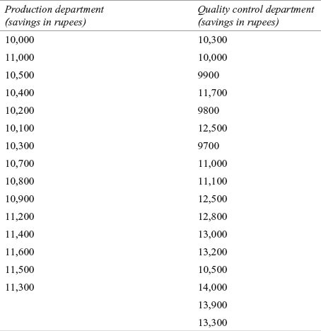
The HR manager of a firm has received a complaint from the employees of the production department that their weekly compensation is less than the compensation of the employees of the marketing department. To verify this claim, the HR manager has taken a random sample of 8 employees from the production department and 9 employees from the marketing department. The data collected are shown in Table 14.2.
Table 14.2 Weekly compensation of the employees of the production and marketing departments

Use the Mann–Whitney U test to determine whether the firm offers different compensation packages to employees of the production and marketing departments. Take α = 0.05 for the test.
Solution The seven steps of hypothesis testing can be performed as below:
Step 1: Set null and alternative hypotheses
H0: The two populations are identical.
H1: The two populations are not identical.
Step 2: Determine the appropriate statistical test
We are not very sure that the distribution of the population is normal. In this case, we will apply the Mann–Whitney U test as an alternative to the t test.
The U statistic for R1 and R2 can be defined as
![]()
and ![]()
Step 3: Set the level of significance
Confidence level is taken as 95% (α = 0.05).
Step 4: Set the decision rule
At 95% (α = 0.05) confidence level, if the p value (double) is less than 0.05, accept the alternative hypothesis and reject the null hypothesis.
Step 5: Collect the sample data
The sample data are as follows:

Step 6: Analyse the data
The test statistic U can be computed as in Table 14.3.
Table 14.3 Weekly compensation (in rupees) of production and marketing department employees with ranks and respective groups

R1 = 1 + 2 + 3 + 6 + 8 + 11 + 12 + 14 = 57
R2 = 4 + 5 + 7 + 9 + 10 + 13 + 15 + 16 + 17 = 96
![]()
![]()
When we compare U1 and U2, we find that U2 is smaller than U1. We have already discussed that test statistic U is the smallest of U1 and U2. Hence, test statistic U is 21.
Step 7: Arrive at a statistical conclusion and business implication
For n1 = 8 and n2 = 9, one-tail p-value is 0.0836 (From the table given in the appendices). For obtaining the two-tail p-value, this one-tail p-value should be multiplied by 2. Hence, for two-tail test, p-value is 0. 0836 × 2 = 0.1672 This p-value is greater than 0.05. So, the null hypothesis is accepted and the alternative hypothesis is rejected. It can be concluded that at 5% level of significance, the two populations are identical.
The complaint from the production department employees that the compensation offered to them is less than the marketing department employees is not genuine (statistically significant). Figures 14.7 and 14.8 are Minitab and SPSS outputs for Example 14.3.

Figure 14.7 Minitab output for Example 14.3

Figure 14.8 SPSS output for Example 14.3
14.3.2 Using Minitab for the Mann–Whitney U Test
The first step is to click Stat/Nonparametrics/Mann-Whitney. The Mann-Whitney dialog box will appear on the screen (Figure 14.9). By using Select, place values of the first sample in the First Sample box, and values of the second sample in the Second Sample box. Place the desired Confidence level in the Confidence level box and select Alternative as not equal. Click OK (as shown in Figure 14.9). Minitab will produce the output as shown in Figure 14.7.
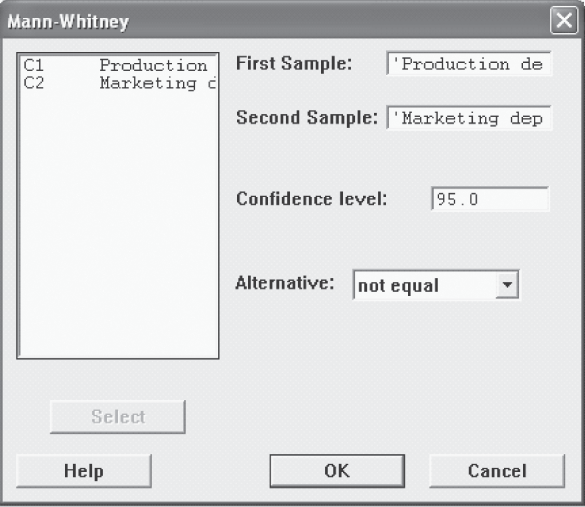
Figure 14.9 Minitab Mann–Whitney dialog box
Note: Minitab tests the alternative hypothesis “two population medians are not equal.” The confidence interval in Figure 14.7 indicates that one is 95.1% confident that the difference between the two population medians is greater than or equal to –379.9 and less than or equal to 49.9. It is important to note that zero is also within the confidence interval. Hence, the null hypothesis cannot be rejected. Therefore, it can be concluded that the two medians are equal.
14.3.3 Using Minitab for Ranking
Minitab can be used for ranking the items very easily. For this, first construct a combined column for production and marketing. The second step is to click Calc/Calculator. The Calculator dialog box will appear on the screen (Figure 14.10). Type Ranking in the “Store result in variable” box and from the Functions box, select Rank and place it in the Expression box. RANK will populate the Expression box. Place Combined besides Rank in the Expression box as shown in Figure 14.10. Click OK. The ranking of columns will be attached with the data sheet under the head Ranking as the output from Minitab.

Figure 14.10 Minitab Calculator dialog box
14.3.4 Using SPSS for the Mann–Whitney U Test
The first step is to click Analyze/Nonparametric/Two-Independent-Sample. The Two-Independent-Samples Tests dialog box will appear on the screen (Figure 14.11). From the Test Type, select, Mann-Whitney U test. Place Departments in the Test Variable List box. Place VAR1 in the Grouping Variable box (Figure 14.12). Click Define Groups. The Two Independent Samples: Define Groups dialog box will appear on the screen (Figure 14.13). Place 1 against Group 1 and place 2 against Group 2 (where 1 represents the production department and 2 represent the marketing department). It is important to note that while feeding the data in SPSS, VAR1 is nothing but the symbolic notations of both the departments in numerical figure, that is, 1 and 2. Figures from the departments (weekly compensation) are placed against 1 and 2 for the production and the marketing department in a vertical column and then titled Departments. After placing 1 and 2 against Group 1 and 2, click Continue. The Two-Independent-Samples Tests dialog box will reappear on the screen with grouping Variable 1 and 2. Click OK. SPSS will produce output as shown in Figure 14.8.
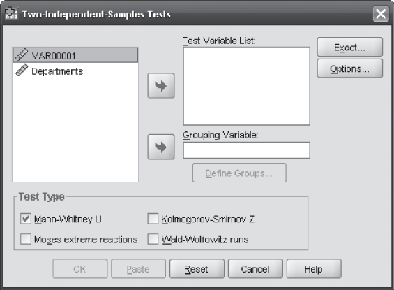
Figure 14.11 SPSS Two-Independent-Samples Tests dialog box
14.3.5 Using SPSS for Ranking
The first step is to construct a combined column for production and marketing. The second step is to click Transform/Rank Cases. The Rank Cases dialog box will appear on the screen (Figure 14.14). Select smallest value from Assigned Rank 1 to check box. Place Departments in the Variable(s) box. Click Rank Types. The Rank Cases: Types dialog box will appear on the screen (Figure 14.15). Select Rank and click Continue from this dialog box. The Rank Cases dialog box will reappear on the screen. Click Ties. The Rank Cases: Ties dialog box will appear on the screen (Figure 14.16). In this dialog box, from Rank Assigned to Ties, select Mean and click Continue. The Rank Cases dialog box will reappear on the screen. Click OK. The ranking of columns will be attached with the data sheet as the output from SPSS.

Figure 14.16 SPSS Rank Cases: Ties dialog box
14.3.6 U Test for Large Samples
When n1(number of items in Sample 1) and n2(number of items in Sample 2) are both greater than 10, the samples are considered to be large samples. In case of large samples, sampling distribution of the U statistic can be approximated by the normal distribution. The z statistic can be computed by using the following formula
When n1(number of items in Sample 1) and n2 (number of items in Sample 2) are both greater than 10, samples are considered to be large samples. In case of large samples, the sampling distribution of the U statistic can be approximated by the normal distribution.
![]()
where mean ![]() and standard deviation
and standard deviation ![]() .
.
The process of using the Mann–Whitney U test, for large samples, can be understood clearly by Example 14.4.
Example 14.4
A manufacturing firm claims that it has improved the saving pattern of its employees, including employees from the production and quality control departments through some special initiatives. The company further claims that it provides equal compensation opportunities to staff from all departments without any discrimination. Therefore, the savings pattern of all employees are the same irrespective of departments. To verify the company’s claim, an investment expert has taken a random sample of size 15 from the production department and a random sample of size 17 from the quality control department. The investment details of employees from the production and quality control departments are given in Table 14.4.
Table 14.4 Investment made by 15 randomly selected employees from the production department and 17 randomly selected employees from the quality control department

Use the Mann–Whitney U test, to determine whether the two populations differ in saving pattern.
Solution The seven steps of hypothesis testing can be performed as below:
Step 1: Set null and alternative hypotheses
H0: The two populations are identical.
H1: The two populations are not identical.
Step 2: Determine the appropriate statistical test
Since we are not very sure that the distribution of the population is normal, we apply the Mann–Whitney U test for large populations
![]()
where mean ![]() and standard deviation
and standard deviation ![]()
Step 3: Determine the level of significance
The confidence level is taken as 95% (α = 0.05).
Step 4: Set the decision rule
At 95% (α = 0.05) confidence level, the critical values are z0.025 = ±1.96. If the computed values are less than –1.96 or greater than +1.96, the decision is to reject the null hypothesis and accept the alternative hypothesis.
Step 5: Collect the sample data
The sample data are given as follows:
Step 6: Analyse the data
The test statistic z can be computed as indicated in Table 14.5.
Table 14.5 Details of the savings made by 15 employees of the production department and 17 employees of the quality control department with ranks and respective groups
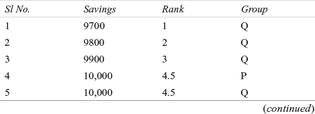

R1 = 4.5 + 6 + 7 + 8.5 + 10 + 11.5 + 13 + 14 + 15 + 16.5 + 19 + 20 + 21 + 22 + 23 = 211
R2 = 1 + 2 + 3 + 4.5 + 8.5 + 11.5 + 16.5 + 18 + 24 + 25.5 + 25.5 + 27 + 28 + 29 + 30 + 31 + 32 = 317
![]()
![]()
When we compare U1 and U2, we find that U2 is smaller than U1. We have discussed earlier that the test statistic U is the smallest of U1 and U2. Hence, the test statistic U is 91.
Mean ![]()
and standard deviation ![]()
![]()
Hence, ![]()
Step 7: Arrive at a statistical conclusion and business implication
The observed value of z is –1.37. This value falls in the acceptance region. Hence, the null hypothesis is accepted and the alternative hypothesis is rejected. It can be concluded that at 5% level of significance, the two populations are identical and they do not differ in savings pattern.
The firm’s claim that since it provides equal compensation to employees of all departments without any discrimination, the savings pattern is also the same for all employees irrespective of the departments can be accepted. Figures 14.17 and 14.18 are the Minitab and SPSS output respectively for Example 14.4.
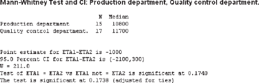
Figure 14.17 Minitab output for Example 14.4
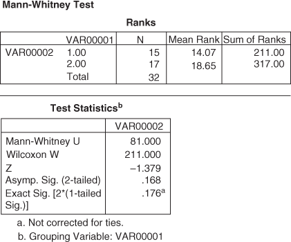
Figure 14.18 SPSS output for Example 14.4
Note: The procedure of using Minitab and SPSS to solve Example 14.4 is the same as the procedure used for Example 14.3.
Self-Practice Problems
14B1. Use Mann–Whitney U test to determine whether there is a significant difference in the data about two groups provided in the table below. Use α = 0.05.
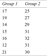
14B2. Use Mann–Whitney U test to determine whether there is a significant difference in the data about two groups provided in the table below. Use α = 0.05.

14.4 Wilcoxon Matched-Pairs Signed Rank Test
The Mann–Whitney U test is an alternative to the t-test to compare the means of two independent populations when the normality assumption of the population is not met or when data are ordinal in nature. There may be various situations when two samples are related. In this case, the Mann–Whitney U test cannot be used. The Wilcoxon test5 is a non-parametric alternative to the t-test for related samples. This test is often described as the non parametric version of paired t-test.6
Wilcoxon test is a non- parametric alternative to the t test for related samples.
The difference scores of two matched groups are computed as the first step for conducting the Wilcoxon test. After computing the difference scores, Rank 1 to n are assigned to the absolute value of the differences. Ranks are assigned from the smallest value to the largest value. Zero difference values are ignored. If the differences are equal, a rank equal to the average of ranks assigned to these values should be assigned. If a difference is negative, the corresponding rank is given a negative sign. This test is called a sign test as it allocates a sign either positive (+) or negative (−) to each observation.7 The next step is to compute the sums of the ranks of positive and negative differences. The sum of positive differences is denoted by T+ and the sum of negative differences is denoted by T–. The Wilcoxon statistic T is defined as the smallest sum of ranks. Symbolically, Wilcoxon statistic T = Minimum of (T+, T–). Similar to the Mann–Whitney U test, different procedures are adopted for small samples and large samples in the Wilcoxon test. When the sample size (number of pairs) is less than or equal to 15 (n ≤ 15), it is treated as a small sample and when the sample size (number of pairs) is greater than 15 (n > 15), it is treated as a large sample.
In the Wilcoxon test, when the sample size (number of pairs) is less than or equal to 15 (n ≤ 15), it is treated as a small sample and when the sample size (number of pairs) is greater than 15 (n > 15), it is treated as a large sample.
The null and alternative hypotheses for the Wilcoxon test can be stated as below:
Hypotheses for a two-tailed test
H0: Md = 0
H1: Md ≠ 0
For one-tailed test (Left tail) For one-tailed test (Right tail)
H0: Md = 0 H0: Md = 0
H1: Md < 0 H1: Md > 0
The decision rules are as below:
For two-tailed test
Reject H0 when T ≤ Tα, otherwise, accept H0.
For one-tailed test
Reject H0 when T– < Tα or T+ < Tα, otherwise, accept H0.
14.4.1 Wilcoxon Test for Small Samples (n ≤ 15)
In case of a small sample, the critical value for which we want to compare T can be found by using n and α. The Wilcoxon test table provided in the appendices can be used for this. For a given sample size n and level of significance α, if the calculated value of T is less than or equal to the tabular (critical) value of T, the null hypothesis is rejected and the alternative hypothesis is accepted. This procedure is explained in Example 14.5.
Example 14.5
A company is trying to improve the work efficiency of its employees. It has organized a special training programme for all employees. In order to assess the effectiveness of the training programme, the company has selected 10 employees randomly and administered a well-structured questionnaire. The scores obtained by the employees are given in the Table 14.6.
Table 14.6 Scores of 10 randomly selected employees before and after training
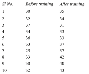
At 95% confidence level, examine whether the training programme has improved the efficiency of employees.
Solution The seven steps of hypothesis testing can be performed as follow:
Step 1: Set null and alternative hypotheses
The hypotheses can be stated as
H0: Md = 0
H1: Md ≠ 0
Step 2: Determine the appropriate statistical test
Since the sample size is less than 15, the small-sample Wilcoxon test will be an appropriate choice.
Step 3: Set the level of significance
Confidence level is taken as 95% (α = 0.05).
Step 4: Set the decision rule
At 95% (α = 0.05) confidence level, the critical value of T is 8. If the computed values are less than or equal to 8, the decision is to reject the null hypothesis and accept the alternative hypothesis.
Step 5: Collect the sample data
The sample data are as follows

Step 6: Analyse the data
The test statistic T can be computed as indicated in Table 14.7.
Table 14.7 Training scores of employees with differences and ranks for before and after the training programme
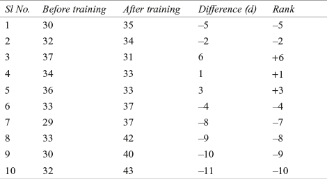
Wilcoxon statistic T = Minimum of (T+, T–)
T+ = 1 + 3 + 6 = 10
T– = 2 + 4 + 5 + 7 + 8 + 9 + 10 = 45
T = Minimum of (T+, T–) = Minimum of (10, 45) = 10
Step 7: Arrive at a statistical conclusion and business implication
At 95% (α = 0.05) confidence level, the critical value of T is 8. The computed value of T is 10 (which is greater than 8); therefore, the decision is to accept the null hypothesis and reject the alternative hypothesis.
We can say that training has not significantly improved the efficiency levels of employees. Figures 14.19 and 14.20 are the Minitab and SPSS output, respectively, for Example 14.5.

Figure 14.19 Minitab output for Example 14.5
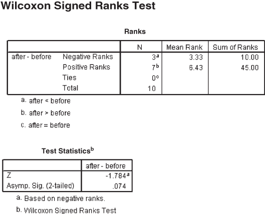
Figure 14.20 SPSS output for Example 14.5
14.4.2 Using Minitab for the Wilcoxon Test
The first step is to click Calc/Calculator. The Calculator dialog box will appear on the screen (Figure 14.21). To create a third column, type “difference” in the Store result in variable box. In the Expression box, place “Before Training”, select a ‘–’ sign and then place ‘After Training’ and click OK. A third column for difference will be created under the column heading “difference.”

Figure 14.21 Minitab Calculator dialog box
The second step is to click Stat/Non parametrics/1-Sample Wilcoxon. The 1-Sample Wilcoxon dialog box will appear on the screen (Figure 14.22). By using Select, place the differences in the Variables box. Select Test Median as 0 and Alternative as not equal and click OK. Minitab will produce the output as shown in Figure 14.19.
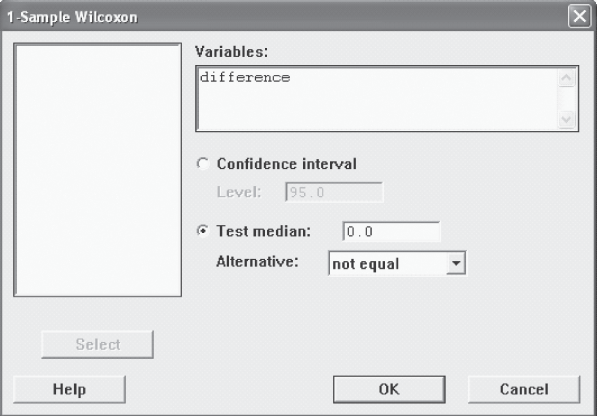
Figure 14.22 Minitab 1-Sample Wilcoxon dialog box
14.4.3 Using SPSS for the Wilcoxon Test
The first step is to click Analyze/Non parametric/Two-Related-Samples. The Two-Related-Samples Tests dialog box will appear on the screen (Figure 14.23). From the Test Type, select Wilcoxon. In the ‘Test Pairs’ box, place before against Variable 1 and place after against Variable 2 (Figure 14.24). Click OK. SPSS will produce the output as shown in Figure 14.20.
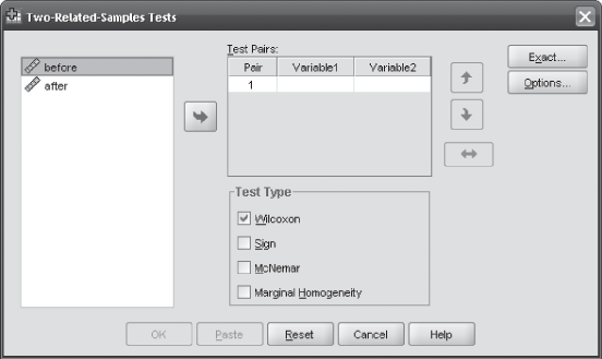
Figure 14.23 SPSS Two-Related-Samples Tests dialog box
14.4.4 Wilcoxon Test for Large Samples (n > 15)
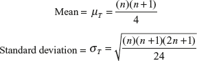
In case of a large sample (n > 15), the sampling distribution of T approaches normal distribution with mean and standard deviation given as below:
Mean = ![]()
Standard deviation = ![]()
The sampling distribution of T approaches normal distribution; hence, the z statistic can be defined as
![]()
where n is the number of pairs and T the Wilcoxon test statistic.
Example 14.6
A software company wants to estimate the change in expenditure of its employees on children’s education in the last five years. The monthly expenditure of 17 randomly selected employees on children’s education in 2000 and 2005 is given in Table 14.8.
Table 14.8 Expenditure of employees (monthly) on children’s education for the year 2000 and 2005 for the software company
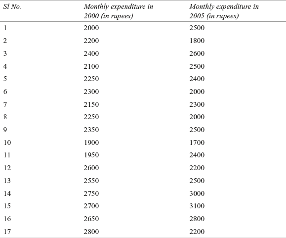
Is there any evidence that there is a difference in expenditure in 2000 and 2005?
Solution The seven steps of hypothesis testing can be performed as below:
Step 1: Set null and alternative hypotheses
The hypotheses can be stated as
H0: Md = 0
H1: Md ≠ 0
Step 2: Determine the appropriate statistical test
The sample size is more than 15. In this case, the large sample Wilcoxon test will be an appropriate choice. The z statistic can be computed by using the following formula:
![]()
Step 3: Set the level of significance
Confidence level is taken as 95% (α = 0.05).
Step 4: Set the decision rule
At 95% (α = 0.05) confidence level, the critical value of z is ±1.96. If the computed value is greater than 1.96 or less than –1.96, the decision is to reject the null hypothesis and accept the alternative hypothesis.
Step 5: Collect the sample data
The sample data are as follows:

Step 6: Analyse the data
The test statistic z can be computed as indicated in Table 14.9.
Table 14.9 Monthly expenditure of 17 randomly selected employees on children’s education in 2000 and 2005 for the software company with difference and rank
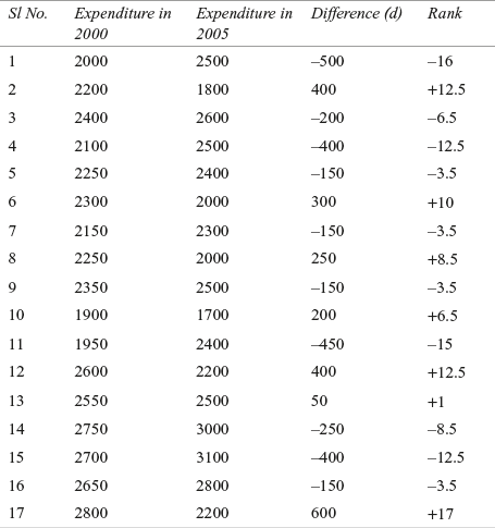
Wilcoxon statistic T = Minimum of (T+, T– )
T+ = 12.5 + 10 + 8.5 + 6.5 + 12.5 + 1 + 17 = 68
T– = 16 + 6.5 + 12.5 + 3.5 + 3.5 + 3.5 + 15 + 8.5 + 12.5 + 3.5 = 85
T = Minimum of (T+, T–) = Minimum of (68, 85) = 68
Mean = ![]()
Standard deviation = ![]()
![]()
Step 7: Arrive at a statistical conclusion and business implication
At 95% confidence level (α = 0.05), the critical value of z is ±1.96. The computed value of z is –0.40 (which falls in the acceptance region). Hence, the decision is to accept the null hypothesis and reject the alternative hypothesis.
There is no evidence of any difference in expenditure for children’s education in 2000 and 2005. Figures 14.25 and 14.26 are the Minitab and SPSS outputs for Example 14.6.

Figure 14.25 Minitab output for Example 14.6
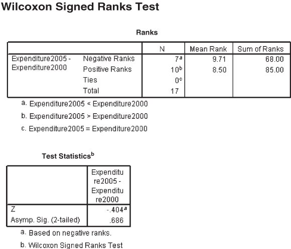
Figure 14.26 SPSS output for Example 14.6
Self-Practice Problems
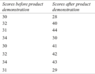
14C1. The table below gives the scores obtained from a random sample of 8 customers before and after the demonstration of a product. Is there any evidence of difference in scores before and after demonstration.
14C2. Use the Wilcoxon test to analyse the following scores obtained from 16 employees (selected randomly) before and after a training programme. Use α = 0.05
14.5 Kruskal–Wallis Test
The Kruskal–Wallis test8 is the non-parametric alternative to one-way ANOVA. There may be cases where a researcher is not clear about the shape of the population. In this situation, the Kruskal–Wallis test is a non-parametric alternative to one-way ANOVA. One-way ANOVA is based on the assumptions of normality, independent groups, and equal population variance. In order to perform one-way ANOVA, it is essential that data is atleast interval scaled. On the other hand, Kruskal–Wallis test can be performed on ordinal data and is not based on the normality assumption of the population. Kruskal–Wallis test is based on the assumption of independency of groups. It is also based on the assumption that individual items are selected randomly. Kruskal–Wallis (KW) test is to be among the most useful of available hypothesis testing procedures for behavioural and social research, though it is also one of the many under-utilized non-parametric procedures.9
Kruskal–Wallis test is the non-parametric alternative to one-way ANOVA.
A researcher has to first draw k independent samples from k different populations. Let these samples of size n1, n2, n3, …, nk be from k different populations. These samples are then combined such that n = n1 + n2 + n3 + ... + nk . The next step is to arrange n observations in an ascending order. The smallest value is assigned Rank 1 and the highest value is assigned the highest rank. In case of a tie, average ranks of ties are assigned. Then ranks corresponding to different samples are added. These totals are denoted by T1, T2, T3, …, Tk. The Kruskal– Wallis statistic is computed by using the following formula
Kruskal–Wallis statistic (K)

where k is the number of groups, n the total number of observations (items), Tj the sum of ranks in a group, and nj the number of observations (items) in a group.
Here, it is important to note that the K value is approximately χ2 distributed with k – 1 degrees of freedom, as long as nj is not less than 5 items for any group.
The null and alternative hypotheses for the Kruskal–Wallis test can be stated as below:
H0: The k different populations are identical.
H1: At least one of the k populations is different.
Decision rule
Reject H0, when the calculated K value > χ2 at k – 1 degrees of freedom and α level of significance, otherwise, accept H0.
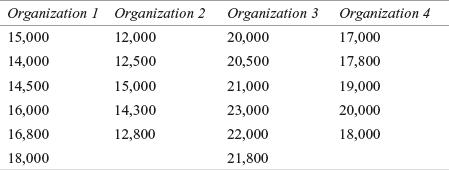
Example 14.7
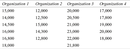
A travel agency wants to know the amount spent by employees of four different organizations on foreign travel. The agency’s researchers have taken random samples from the four organizations. The amount spent is given in Table 14.10. Use the Kruskal–Wallis test to determine whether there is a significant difference between employees of organizations in terms of the amount spent on foreign travel. Use α = 0.05
Table 14.10 Expenditure on foreign travel by employees of four organizations
Solution The seven steps of hypothesis testing can be performed as below:
Step 1: Set null and alternative hypotheses
The null and alternative hypotheses can be stated as below:
H0: The k different populations are identical.
H1: At least one of the k populations is different.
Step 2: Determine the appropriate statistical test
The Kruskal–Wallis statistic is the appropriate test statistic.
Step 3: Set the level of significance
Confidence level is taken as 95% (α = 0.05).
Step 4: Set the decision rule
In this example, degrees of freedom is k – 1 = 4 – 1 = 3. At 95% confidence level and 3 degrees of freedom, the critical value of chi-square is ![]() Reject H0 when the calculated K value > 7.8147.
Reject H0 when the calculated K value > 7.8147.
Step 5: Collect the sample data
The sample data are as follows:
Step 6: Analyse the data
The test statistic K can be computed as indicated in Table 14.11.
Table 14.11 Computation of rank total for determining the significant difference in the amount spent on travel by the employees of four organizations
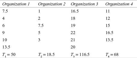
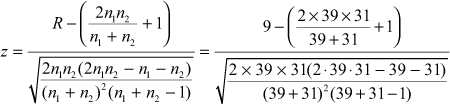
Kruskal–Wallis statistic (K)
where 
![]()
Step 7: Arrive at a statistical conclusion and business implication
At 95% confidence level and 3 degrees of freedom, the critical value of chi-square is ![]() Reject H0, when the calculated K value > 7.8147. The calculated K value is 18.08, which is greater than 7.8147. Hence, the null hypothesis is rejected and the alternative hypothesis is accepted. Here, it is important to note that the test is always one-tailed and rejection region will always be in the right tail of the distribution.
Reject H0, when the calculated K value > 7.8147. The calculated K value is 18.08, which is greater than 7.8147. Hence, the null hypothesis is rejected and the alternative hypothesis is accepted. Here, it is important to note that the test is always one-tailed and rejection region will always be in the right tail of the distribution.
On the basis of the test result, it can be concluded that the amount spent by employees of the four organizations on foreign travel is different. So, the travel company should chalk out different plans for different organizations. Figures 14.27 and 14.28 are the Minitab and SPSS output, respectively for Example 14.7
14.5.1 Using Minitab for the Kruskal–Wallis Test
In the Kruskal–Wallis test, the data are arranged in the Minitab worksheet in a different manner (shown in Figure 14.29). It can be noticed that all the organizations are placed in one column with different treatment levels (in this example, it is 1, 2, 3, and 4, for four different organizations). The corresponding amount is placed in the second column. The next step is to click Stat/Nonparametrics/Kruskal-Wallis. The Kruskal-Wallis dialog box will appear on the screen (Figure 14.30). Place Organizations in the Factor box and “Amount spent” in the Response box. Click OK. The Minitab output (as shown in Figure 14.27) will appear on the screen.
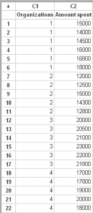
Figure 14.29 Arrangement of data for Example 14.7 in the Minitab worksheet

Figure 14.30 Minitab Kruskal–Wallis dialog box
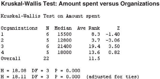
Figure 14.27 Minitab output for Example 14.7

Figure 14.3 Minitab Runs Test dialog box
14.5.2 Using SPSS for the Kruskal–Wallis Test
The first step is to click Analyze/Nonparametric/K Independent Samples. The Tests for Several Independent Samples dialog box will appear on the screen (Figure 14.31). From the Test Type, select Kruskal–Wallis H (Figure 14.31). Place AmtSpent in the Test Variable List and Organizations in the Grouping Variable box. Click Define Range; The Several Independent Samples: Define Range dialog box will appear on the screen (Figure 14.32). In the Range for Grouping Variable box, place 1 against Minimum and 4 against Maximum as shown in Figure 14.32. Click Continue. The Tests for Several Independent Samples dialog box will reappear on the screen. Click OK. SPSS will produce the output as shown in Figure 14.28.

Figure 14.28 SPSS output for Example 14.7
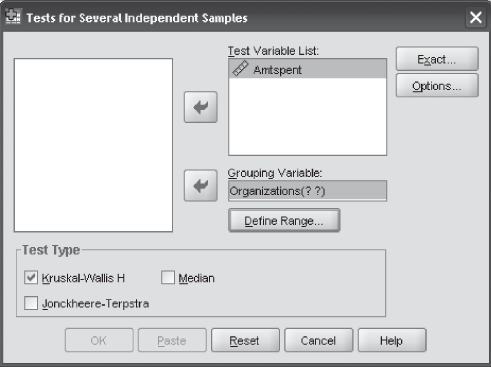
Figure 14.31 SPSS Tests for Several Independent Samples dialog box
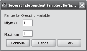
Figure 14.32 SPSS Several Independent Samples: Define Range dialog box
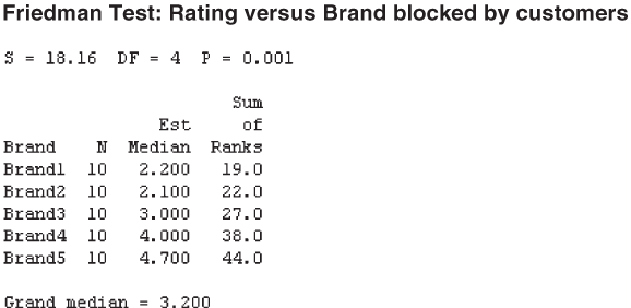
Figure 14.33 Minitab output for Example 14.8
Self-Practice Problems
14D1. The following table provides the yearly savings of employees (in thousand rupees) selected randomly from four organizations. Use the Kruskal–Wallis test to determine whether there is a significant difference in the savings of employees of the four organizations.

14.6 Friedman Test
Friedman test10 is the non-parametric alternative to randomized block design. Developed by M. Friedman in 1937, the Friedman test is used when assumptions of ANOVA are not met or when researchers have ranked data.11 In fact, the Friedman test is very useful when data are ranked within each block. The Friedman test is based on the following assumptions:
- 1. The blocks are independent.
- 2. There is no interaction between blocks and treatments.
- 3. Observations within each block can be ranked.
The null and alternative hypotheses in the Friedman test can be set as
H0 : The distribution of k treatment populations are identical.
H1 : All k treatment populations are not identical.
The first step in the Friedman test is to rank data within each block from 1 to k (unless the data are already ranked). In other words, the smallest item in the block gets the Rank 1, second smallest item in the block gets the Rank 2, and the highest value gets the Rank k. After assigning ranks to the items of all the blocks, the ranks pertaining to treatment (columns) are summed. The sum of all the ranks for Treatment 1 is denoted by R1 and is denoted by R2 for Treatment 2 and so on. As the null hypothesis states that the distribution of k treatment populations are identical, then the sum of ranks obtained from one treatment will not be very different from the sum of ranks obtained from other treatments. This difference among the sum of ranks between various treatment is measured by the Friedman test statistic and denoted by ![]() . The formula used for calculating this test statistic can be stated as
. The formula used for calculating this test statistic can be stated as
Friedman test statistic
![]()
where k is the number of treatment levels (columns), b the number of blocks (rows), ![]() the rank total for a particular treatment (column), and j the particular treatment level.
the rank total for a particular treatment (column), and j the particular treatment level.
The Friedman test statistic described above is approximately χ2 distributed, with degrees of freedom = k – 1 when k > 4 or when k = 3 and b > 9 or when k = 4 and b > 4. For small values of k and b, tables of the exact distribution of χ2 may be found in some specific books based on non-parametric statistics. Example 14.8 explains the procedure of conducting the Friedman test.
Example 14.8
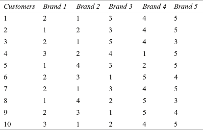
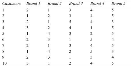
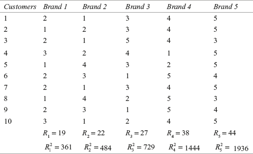
A two-wheeler manufacturing company wants to assess the satisfaction level of customers with its latest brand as against their satisfaction with four other leading brands. Researchers at the company have selected 8 customers randomly and asked them to rank their satisfaction levels on a scale from 1 to 5. The results are presented in Table 14.12. Determine whether there is any significant difference between the ranking of brands. Use α = 0.05

Figure 14.12 SPSS Two-Independent-Samples Tests dialog box (after placing departments in the Test Variable List box and Variable 1 in the Grouping Variable box)
Table 14.12 Ranking of satisfaction levels of eight randomly selected customers
Solution The seven steps of hypothesis testing can be performed as below:
Step 1: Set null and alternative hypotheses
The null and alternative hypotheses can be stated as below:
H0 : The distribution of the population of five brands are identical.
H1 : The distribution of the population of five brands are not identical.
Step 2: Determine the appropriate statistical test
The Friedman test statistic is the appropriate test statistic.
Step 3: Set the level of significance
The confidence level is taken as 95% (α = 0.05).
Step 4: Set the decision rule
In this example, degrees of freedom is k – 1 = 5 – 1 = 4. At 95% confidence level and 4 degrees of freedom, the critical value of chi-square is ![]() Reject H0, when the calculated
Reject H0, when the calculated ![]() value > 9.4877.
value > 9.4877.
Step 5: Collect the sample data
The sample data are as follows:
Step 6: Analyse the data
The test statistic ![]() can be computed as indicated in Table 14.13.
can be computed as indicated in Table 14.13.
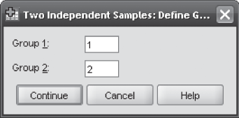
Figure 14.13 SPSS Two Independent Samples: Define Groups dialog box
Table 14.13 Computation of the rank total and rank total square for determining the significant difference between the ranking of brands by eight randomly selected customers
The Friedman test statistic is given as
![]()
where
![]()
![]()
Step 7: Arrive at a statistical conclusion and business implication
At 95% confidence level and 4 degrees of freedom, the critical value of chi-square is ![]() The calculated value of
The calculated value of ![]() is greater than the critical value of chi-square. Hence, the null hypothesis is rejected and the alternative hypothesis is accepted.
is greater than the critical value of chi-square. Hence, the null hypothesis is rejected and the alternative hypothesis is accepted.
On the basis of the test results, it can be concluded that there is a significant difference between the rankings of brands. So, the two-wheeler manufacturing company can decide on its marketing strategies according to the different levels of consumer satisfaction. Figures 14.33 and 14.34 are Minitab and SPSS output respectively, for Example 14.8.
14.6.1 Using Minitab for the Friedman Test
Like the Kruskal–Wallis test, the arrangement of data in the Minitab worksheet for the Friedman test follows a different style (shown in Figure 14.35). It can be noticed that all the customers are placed in the first column and ranking and brands are placed in the second and third columns, respectively.

Figure 14.35 Arrangement of data for Example 14.8 in Minitab worksheet
The next step is to click Stat/Nonparametrics/Friedman. The Friedman dialog box will appear on the screen (Figure 14.36). Place columns, related to Ranking, Brand, and Customers in Response, Treatment, and Blocks boxes, respectively. Click OK, the Minitab output as shown in Figure 14.33 for Example 14.8, will appear on the screen.

Figure 14.36 Minitab Friedman dialog box
14.6.2 Using SPSS for the Friedman Test
The first step is to click Analyze/Nonparametric/K Related-Samples. The Tests for Several Related Samples dialog box will appear on the screen (Figure 14.37). From the Test Type, select Friedman and place all the brand columns in the Test Variables box (Figure 14.37). Click OK, SPSS output for Example 14.8 will appear on the screen (Figure 14.34).

Figure 14.34 SPSS output for Example 14.8

Figure 14.37 SPSS Tests for Several Related Samples dialog box

Self-Practice Problems
14E1. A researcher has gathered information from 8 randomly selected officers, on how they spend money on five parameters: children’s education, house purchase, recreation, out-of-city tour on vacation, and savings for the future. The ranking obtained are presented in the table below. Determine whether there is any significant difference between the ranking of individuals on different parameters. Use α = 0.05.
14.7 Spearman’s Rank Correlation
It has been discussed in the previous chapter that the Pearson correlation coefficient r measures the degree of association between two variables. When data is of ordinal level (ranked data), the Pearson correlation coefficient r cannot be applied. In this case, Spearman’s rank correlation12 can be used to determine the degree of association between two variables. The Spearman’s rank correlation was developed by Charles E. Spearman (1863–1945). Spearman’s Rank Correlation coefficient rho is a non-parametric measure of association to have featured in most modern courses, textbooks and computer packages in elementary statistics.13 It can be calculated by using the following formula:
Spearman’s rank correlation
![]()
where n is the number of paired observations and d the difference in ranks for each pair.
When data is of ordinal level (ranked data), Pearson correlation coefficient r cannot be applied. In this case, Spearman’s rank correlation can be used to determine the degree of association between two variables.
The process of computing Spearman’s rank correlation starts with assigning ranks within each group. The difference between the ranks of the items of the first group and corresponding rank of the items of the second group is computed and is generally denoted by d. This difference (d) is squared and then its sum is obtained. n is the number of pairs in the group.
It is very important to understand that the interpretation of Spearman’s rank correlation (rs) is similar to the interpretation of Pearson correlation coefficient r. Correlation near +1 indicates a high degree of positive correlation, correlation near –1 indicates a high degree of negative correlation and correlation near 0 indicates no correlation between two variables.
Example 14.9
A social science researcher wants to find out the degree of association between sugar prices and wheat prices. The researcher has collected data relating to the price of sugar and wheat in 14 randomly selected months from the last 20 years. How can he compute the Spearman’s rank correlation from the data provided in Table 14.14.

Figure 14.14 SPSS Rank Cases dialog box
Table 14.14 Sugar and wheat prices for 14 randomly selected months from the last 20 years

Solution In this example, n = 14. The researcher has to prepare Table 14.15 to first calculate the ranks of individual items in a group and then find out the difference between ranks, the square of this difference and the sum as shown in Table 14.15.

Figure 14.15 SPSS Rank Cases: Types dialog box
Table 14.15 Computation of ranks of sugar and wheat prices, difference between ranks, square of the difference and summation

Spearman’s rank correlation
![]()
14.7.1 Using SPSS for Spearman’s Rank Correlation
The first step is to click Analyze/Correlate/Bivariate. The Bivariate Correlation dialog box will appear on the screen (Figure 14.38). In this dialog box, from the Correlation Coefficients, select Spearman and from Test of Significance, select Two-tailed. Select “Flag significant correlations.” Place variables in the Variables box and click OK. The SPSS output for Example 14.9 will appear on the screen (Figure 14.39). In the output generated by SPSS, the level of significance is also exhibited.
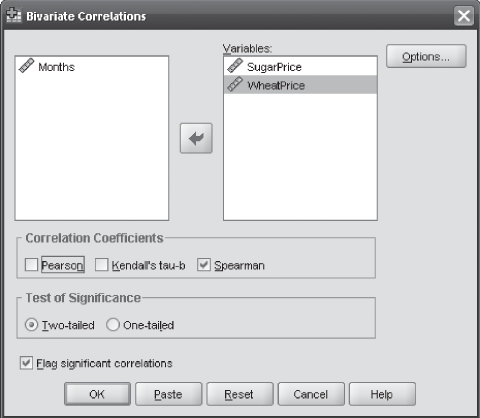
Figure 14.38 SPSS Bivariate Correlations dialog box
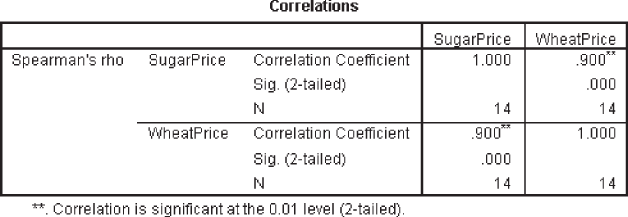
Figure 14.39 SPSS output for Example 14.9
Figure 14.40 SPSS output for Example 14.10
Self-Practice Problems
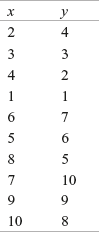
14F1. The following table shows the ranks of the values of two variables x and y. Compute the Spearman’s rank correlation from the data.
14F2. The table below shows the monthwise international price of coconut oil (in US $ per metric tonne) from January 1990 to January 2006 and February 1990 to February 2006. Compute Spearman’s rank correlation from the data.
Monthwise international price of coconut oil (in US $ per metric tonne) from January 1990–January 2006 and February 1990–February 2006

Source: www.indiastat.com, accessed January 2009, reproduced with permission.
Example 14.10
The usage of microwave ovens has increased over the years. 40% of the cons-umers use 27 and 37 litres capacity microwave ovens.4 A researcher who isdoubtful about the accuracy of this figure surveyed 70 randomly sampled microwave oven users. He asked a question, “Do you have 27 and 37 litres capacity microwave ovens?.” The sequence of responses to this ques-tion is given below with Y denoting Yes and N denoting No.Use the runstest to determine whether this sequence is random. Use α = 0.05.
Y,Y,Y,Y,Y,Y,Y,Y,Y,Y,N,N,N,N,N,N,N,N,N,N,Y,Y,Y,Y,Y,Y,Y,Y,N,N,N,N,N,N,Y,Y,Y, Y,Y,Y,Y,Y,Y,N,N,N,N,N,N,N,N,Y,Y,Y,Y,Y,Y,Y,N,N,N,N,N,N,N,Y,Y,Y,Y,Y
Solution The hypotheses to be tested are as follows:
H0 : The observations in the samples are randomly generated.
H1 : The observations in the samples are not randomly generated.
At 95% (α = 0.05) confidence level and for a two-tailed test ![]() , the critical values are z0.025 = ±1.96. If the computed value of z is greater than +1.96 and less than –1.96, the null hypothesis is rejected and the alternative hypothesis is accepted.
, the critical values are z0.025 = ±1.96. If the computed value of z is greater than +1.96 and less than –1.96, the null hypothesis is rejected and the alternative hypothesis is accepted.
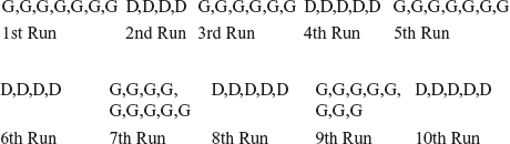
In this example, the number of runs are 9 as shown below
Y,Y,Y,Y,Y,Y,Y,Y,Y,Y N,N,N,N,N,N,N,N,N,N Y,Y,Y,Y,Y,Y,Y,Y
1st Run 2nd Run 3rd Run
N,N,N,N,N,N Y,Y,Y,Y,Y,Y,Y,Y,Y N,N,N,N,N,N,N,N
4th Run 5th Run 6th Run
Y,Y,Y,Y,Y,Y,Y N,N,N,N,N,N,N Y,Y,Y,Y,Y
7th Run 8th Run 9th Run
The test statistic z can be computed as follows:
![]()
The z value is computed as –6.47, which falls in the rejection region. Hence, the null hypothesis is rejected and the alternative hypothesis is accepted. Figure 14.40 shows the SPSS output for Example 14.10. The p value observed from the figure also indicates the rejection of the null hypothesis and the acceptance of the alternative hypothesis. It can be concluded with 95% confidence that observations in the sample are not randomly generated.

Example 14.11
A departmental store wants to open a branch in a rural area. The chief manager of the departmental store wants to know the difference between the income of rural and urban households per month for this purpose. An analyst of the firm has taken a random sample of 13 urban households and 13 rural households and the information obtained is presented in Table 14.16. Use the Mann–Whitney U test to determine whether there is a significant difference between urban and rural household income. Use α = 0.05
Table 14.16 Random sample of 13 urban households and 13 rural households indicating monthly income (in thousand rupees)

Solution As discussed in the chapter, the null and alternative hypotheses can be framed as
H0: The two populations are identical.
H1: The two populations are not identical.
The test statistic U can be computed as indicated in Table 14.17.
Table 14.17 Income of 13 randomly selected urban and rural households (as combined series) with rank and respective groups

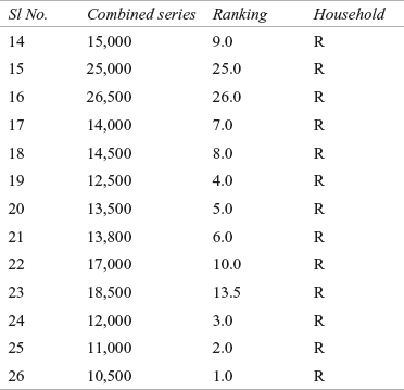
R1 = 24 + 22 + 11 + 13.5 + 17.5 + 21 + 12 + 15.5 + 20 + 19 + 15.5 + 17.5 + 23 = 231.5
R2 = 9 + 25 + 26 + 7 + 8 + 4 + 5 + 6 + 10 + 13.5 + 3 + 2 + 1 = 119.5
![]()
![]()
When we compare the values of U1 and U2, we find that U1 is the smaller value. We know that the test statistic U is the smaller of the values of U1 and U2. Hence, the test statistic U is 28.5.
Mean ![]()
and standard deviation
![]()
Hence, ![]()
At 95% confidence level, the z value falls in the rejection region. Hence, the null hypothesis is rejected and the alternative hypothesis is accepted. At 95% confidence level, the two populations are not identical and a difference exists in the income of urban and rural households. Figure 14.41 exhibits the SPSS output for Example 14.11. The p value shows in Figure 14.41 also indicates the acceptance of the alternative hypothesis.
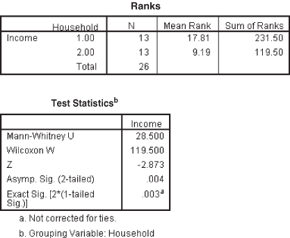
Figure 14.41 SPSS output for Example 14.11
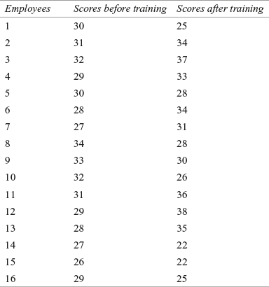
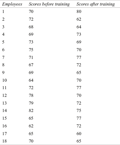
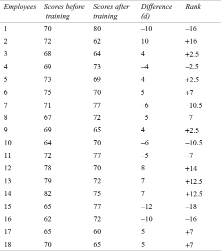
Example 14.12
A company has organized a special training programme for its employees. Table 14.18 provides the scores of 18 randomly selected employees before and after the training programme. Use the Wilcoxon test to find the difference in scores before and after the training programme. Use α = 0.05
Table 14.18 Before and after training scores of 18 randomly selected employees
Solution The null and alternative hypotheses can be framed as below:
H0: Md = 0
H1: Md ≠ 0
The Wilcoxon statistic T can be computed as indicated in Table 14.19. The Wilcoxon statistic T is defined as the minimum of T+ and T–.
Table 14.19 Before and after training scores of 18 randomly selected employees with differences and ranks
Wilcoxon statistic T = Minimum of (T+, T– )
T+ = 16 + 2.5 + 2.5 + 7 + 2.5 + 14 + 12.5 + 12.5 + 7 + 7 = 83.5
T– = 16 + 2.5 + 10.5 + 7 + 10.5 + 7 + 18 + 16 = 87.5
T = Minimum of (T+, T–) = Minimum of (83.5, 87.5) = 83.5
Mean = ![]()
Standard deviation =
![]()
![]()
At 95% (α = 0.05) confidence level, the critical value of z is ±1.96. The computed value of z is –0.08 (which falls in the acceptance region). Hence, the decision is to accept the null hypothesis and reject the alternative hypothesis. Figure 14.42 is the SPSS output for Example 14.12. The p value also indicates the acceptance of the null hypothesis and the rejection of the alternative hypothesis. Hence, there is no evidence of any difference in scores before and after the training programme.
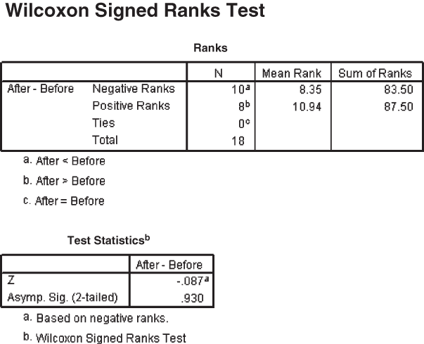
Figure 14.42 SPSS output for Example 14.12
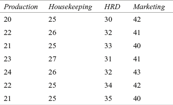
Example 14.13
A company is concerned about its workers devoting more time than necessary to paper work. The company’s researcher has taken a random sample of 8 employees from four major departments: production, housekeeping, HRD, and marketing to test this. The researcher has collected data on weekly hours spent on paper work by the employees as presented in Table 14.20. Use the Kruskal–Wallis test to determine whether there is a significant difference in the weekly hours spent by the employees of the four departments on completing paper work.
Table 14.20 Weekly hours spent on completing paper work by the employees of four different departments
Solution The null and alternative hypotheses can be stated as below:
H0: The k different populations are identical.
H1: At least one k population is different.
The Kruskal–Wallis statistic (K) can be computed by first computing the ranks of values given in Table 14.20.
Table 14.21 Ranking of the hours spent on paper work by the employees of different departments

As discussed in the chapter, the Kruskal–Wallis statistic (K) is defined as below:

where 
![]()
At 95% confidence level and 3 degrees of freedom, the critical value of chi-square is ![]() Reject H0 when the calculated K value > 7.8147. The calculated K value is 25.34, which is greater than 7.8147. Hence, the null hypothesis is rejected and the alternative hypothesis is accepted. Figure 14.43 is the Minitab output for Example 14.13. The p value also indicates the acceptance of the alternative hypothesis and the rejection of the null hypothesis.
Reject H0 when the calculated K value > 7.8147. The calculated K value is 25.34, which is greater than 7.8147. Hence, the null hypothesis is rejected and the alternative hypothesis is accepted. Figure 14.43 is the Minitab output for Example 14.13. The p value also indicates the acceptance of the alternative hypothesis and the rejection of the null hypothesis.
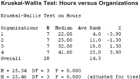
Figure 14.43 Minitab output for Example 14.13
Example 14.14
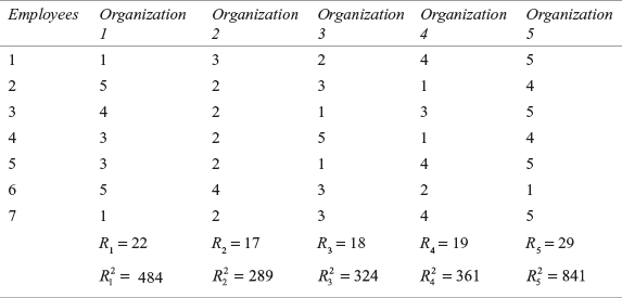
A company wants to assess the outlook of its employees towards five organizations on the criteria “organizational effectiveness.” The company has taken a random sample of 7 employees to obtain the ranking of the five organizations. The scores obtained are given in Table 14.22. Determine whether there is a significant difference between the ranking of organizations. Use α = 0.05
Table 14.22 Outlook of employees towards five organizations on the criteria organizational effectiveness

Solution The null and alternative hypotheses can be stated as below:
H0: The population of the five organizations are identical.
H1: The population of the five organizations are not identical.
The test statistic ![]() can be computed as indicated in Table 14.23.
can be computed as indicated in Table 14.23.
Table 14.23 Outlook of employees towards five organizations on the criteria organizational effectiveness with the sum of ranks and their squares
Friedman test statistic
![]()
where
![]()
![]()
At 95% confidence level and 4 degrees of freedom, the critical value of chi-square is ![]() The calculated value of
The calculated value of ![]() is less than the critical value of chi-square. Hence, the null hypothesis is accepted and the alternative hypothesis is rejected. Figure 14.44 is the SPSS output for Example 14.14.
is less than the critical value of chi-square. Hence, the null hypothesis is accepted and the alternative hypothesis is rejected. Figure 14.44 is the SPSS output for Example 14.14.
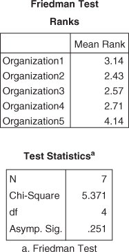
Figure 14.44 SPSS output for Example 14.14
Example 14.15
Madras Cement Ltd is a cement manufacturer based in south India. Table 14.24 provides the profit after tax (in million rupees) and expenses (in million rupees) of Madras Cement Ltd from 1994–1995 to 2006–2007. Compute the Spearman’s rank correlation from the data given in Table 14.24.

Figure 14.24 SPSS Two-Related-Samples Tests (placement of before and after in Current Selections) dialog box
Table 14.24 Profit after tax (in million rupees) and expenses (in million rupees) of Madras Cement Ltd from 1994–1995 to 2006–2007

Source: Prowess (V. 3.1), Centre for Monitoring Indian Economy Pvt. Ltd, Mumbai, accessed January 2009, reproduced with permission.
Solution Table 14.25 exhibits computation of rank and its difference for computing Spearman’s rank correlation for the data given in Table 14.24
Table 14.25 Ranks and the difference in ranks for computing Spearman’s rank correlation coefficient

Spearman’s rank correlation
![]()
Figure 14.45 shows the SPSS output for Example 14.15.

Figure 14.45 SPSS output for Example 14.15
Endnotes |
1. Feys, J. (2016). “Non-Parametric Tests for the Interaction in Two-Way Factorial Designs Using R,” The R Journal, 8(1): 367–378.
2. Hui, W., Y.R. Gel and J.S. Gastwirth (2008). “Lawstat: An R Package for Law, Public Policy and Biostatistics,” Journal of Statistical Software, 28(3):1–26.
3. Mann, H.B. and D. R. Whitney (1947). “On a Test of Whether One of Two Random Variables Is Stochastically Larger than the Other,” Annals of Mathematical Statistics, 18(1):50–60.
4. Nachar, N. (2008). “The Mann–Whitney U: A Test for Assessing Whether Two Independent Samples Come from the Same Distribution,” Tutorials in Quantitative Methods for Psychology, 4(1):13–20.
5. Wilcoxon, F. (1945). “Individual Comparisons by Ranking Methods,” Biometrics Bulletin, 1 (6): 80–83.
6. Kerby, D.S. (2014). “The Simple Difference Formula: An Approach to Teaching Nonparametric Correlation,” Innovative Teaching, 3(1):1–9.
7. Whitley, E. And J. Ball (2002). “Statistics Review 6: Nonparametric Methods,” Critical Care, 6(6):509–513.
8. Kruskal, W. (1952). “Use of Ranks in One-Criterion Variance Analysis,” Journal of the American Statistical Association, 47 (260): 583–621.
9. Elamir, E.A.H. (2015). “Kruskal–Wallis Test: A Graphical Way,” International Journal of Statistics and Applications, 5(3): 113–119.
10. Friedman, M. (1937). “The Use of Ranks to Avoid the Assumption of Normality Implicit in the Analysis of Variance,” Journal of the American Statistical Association, 32 (200): 675–701.
11. Hager, W. (2007). “Some Common Features and Some Differences between the Parametric ANOVA for Repeated Measures and the Friedman ANOVA for Ranked Data,” Psychology Science, 49(3): 209–222.
12. Spearman, C. (1904). “The Proof and Measurement of Association between Two Things,” American Journal of Psychology, 15: 72–101.
13. Lovie, A.D. (1995). “Who Discovered Spearman’s Rank Correlation?” British Journal of Mathematical and Statistical Psychology, 48(2): 225–269
SUMMARY |
Parametric tests are statistical techniques to test a hypothesis based on some assumptions about the population. In some cases, a researcher finds that the population is not normal or the data being measured is qualitative in nature. In these cases, researchers cannot apply parametric tests for hypothesis testing and have to use non-parametric tests. Some of the commonly used and important non-parametric tests are: runs test for randomness of data; the Mann–Whitney U test; the Wilcoxon matched-pairs signed rank test; the Kruskal–Wallis test; the Friedman test, and the Spearman’s rank correlation.
The runs test is used to test the randomness of the samples. The Mann–Whitney U test is an alternative to the t-test to compare the means of two independent populations when the normality assumption of population is not being met or when the data are ordinal in nature. There may be various situations, when two samples are related. In this case, the Mann–Whitney U test cannot be used. The Wilcoxon test is a non-parametric alternative to the t-test for related samples. The Kruskal– Wallis test is the non-parametric alternative to one-way analysis of variance. Kruskal-Wallis test can be performed on ordinal data and is not based on the normality assumption of the population. The Friedman test is the non-parametric alternative to randomized block design. When data are of ordinal level (ranked data), Pearson correlation coefficient r cannot be applied. In this case, Spearman’s rank correlation can be used to determine the degree of association between two variables.
Key terms |
Friedman test, 442
Kruskal–Wallis Test, 436
Mann–Whitney U test, 413
Non-parametric tests, 406
Run test, 407
Spearman’s rank Correlation, 438
Wilcoxon test, 427
notes |
- 1. www.bajajelectricals.com/default.aspx, accessed September 2008.
- 2. Prowess (V. 3.1), Centre for Monitoring Indian Economy Pvt. Ltd, Mumbai, accessed September 2008, reproduced with permission.
- 3. www.bajajelectricals.com/t-wculture.aspx, accessed September 2008.
- 4. www.indiastat.com, accessed September 2008, reproduced with permission.
Discussion questions |
- 1. What is the difference between parametric tests and non-parametric tests? Discuss in the light of how these tests are used in marketing research.
- 2. Explain the major advantages of non-parametric tests over parametric tests.
- 3. What are the main problems a researcher faces when he applies non-parametric tests?
- 4. How can a researcher use the runs test to test the random-ness of samples?
- 5. What is the concept of the Mann–Whitney U test and in what circumstances can it be used?
- 6. Which test is the non-parametric alternative to the t-test for related samples and what are the conditions for its application?
- 7. What is the concept of the Kruskal–Wallis test?
- 8. What is the concept of the Friedman test? How can a researcher use the Friedman Test as a non-parametric alternative to randomized block design?
- 9. Which test is used to determine the degree of association between two variables when data are of ordinal level (ranked data).
Formulas |
Large sample run test:
Mean of the sampling distribution of the R statistic
![]()
Standard deviation of the sampling distribution of the R statistic

Mann–Whitney U test:
Small sample U test

Large sample U Test
![]()
where mean ![]() and standard deviation σU =
and standard deviation σU = ![]()
Wilcoxon matched-pairs signed rank test:
Wilcoxon test for large samples (n > 15)
![]()
where n is the number of pairs and T the Wilcoxon test statistic.
Kruskal–Wallis statistic (K)
![]()
where k is the number of groups, n the total number of observations (items), Tj the sum of ranks in a group and nj the number of observations (items) in a group.
Friedman test statistic
![]()
where k is the number of treatment levels (columns), b the number of blocks (rows) ![]() the rank total for a particular treatment (column), and j the particular treatment level.
the rank total for a particular treatment (column), and j the particular treatment level.
Spearman’s rank correlation
![]()
where n is the number of paired observations and, d the difference in ranks for each pair of observation.
Numerical problems |
- 1. A quality control inspector has discovered that a newly installed machine is producing some defective products. He has obtained 22 products selected randomly from the machine operator to check this. The operator has given him 22 products as below:
F,F,F,F,R,R,R,R,F,F,F,F,R,R,R,R,F,F,F,F,R,R
F indicates a flawed product and R indicates a good product. After a cursory inspection, the quality control inspector feels that the samples are not randomly selected samples. How will he confirm whether these samples were randomly selected?
- 2. A manufacturing process produces good parts and defective parts. A quality control inspector has examined 53 products for defective parts. Good (G) and defective (D) parts are randomly sampled in the following manner:
G,G,G,G,G,G,G,D,D,D,G,G,G,G,G,D,D,D,D,G,G,G,G,G, G,G,D,D,D,D,G,G,G,G,G,G,G,D,D,D,D,G,G,G,G,G,G, D,D,D,D,D,D
Use α = 0.05, to determine whether the machine operator has selected the samples randomly.
- 3. Following are the two random samples gathered from two populations. Use the Mann–Whitney U test to determine whether these two populations differ significantly. Use α = 0.05.

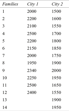
- 4. A researcher wants to know the difference in the monthlyhousehold expenditure on grocery items in two cities. The researcher has randomly selected 12 families from city 1 and 14 families from city 2. Use an appropriate test to determine whether there is a significant difference between families of two cities on the amount spent on grocery items.
- 5. A company has invested heavily on advertisements for a particular brand. The company wants to estimate the impact of advertisements on sales. The company’s researchers have randomly selected 10 dealers. They noted the sales of these dealers before and after implementing the advertisement campaign. The sales data for the periods before and after the investment on advertisement are given in the table below. Use the Wilcoxon matched-pairs signed rank test to determine the difference in sales before and after the investment on advertisement. Use α = 0.10.
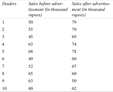
- 6. A watch manufacturer has launched a number of service improvement programmes for improving the quality of its services. The company wants to estimate whether the satisfaction level of its customers has improved after the programme has been implemented for two years. The company had taken a random sample of 18 customers, and obtained scores from these customers in 2004 (before service improvement programme) and 2006 (after service improvement programme). The table below provides the scores given by customers in 2004 and 2006. Use the Wilcoxon matched-pairs signed rank test to determine the difference in scores obtained from customers before and after launching the service improvement programme. Use α = 0.05.

- 7. Employees of Organization 1 claim that the night shift payment they receive is different from the payment received by employees working in the same industry. For checking the validity of this claim, researchers of the company have collected data from three organizations (including Organization 1) in the same industry. The amount received by different randomly sampled employees of these three organizations per night shift is tabulated below:
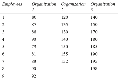
Use the Kruskal–Wallis test to determine whether there is a significant difference between employees of organizations in terms of night shift payment. Use α = 0.05.
- 8. A chemical company is facing the problem of high employee turnover. Job dissatisfaction has been attributed as the primary reason behind the high turnover rate. Company management has decided to measure the degree of job satisfaction of its employees compared to employees of four other organizations from the same industry. The company has appointed a professional research group and its researchers have taken a random sample of 10 employees from each organization and used a well-structured questionnaire with 10 question on a five-point rating scale. Scores obtained by the employees are given in the table below. Determine if there are significant differences between job satisfaction levels of employees. Use α = 0.05 In the table, Org 1is the chemical company, which is facing high turnover of employees and Org 2, Org 3, Org 4 and Org 5 are the other four organizations.

- 9. A researcher wants to know the degree of association between petrol and diesel prices. For this, researcher has selected a random sample of 10 month’s price of petrol and diesel from the last 20 years. How can he compute the Spearman’s rank correlation from the following table:

Case study |
Case 14: Indian Aviation Industry: Jet Airways (India) Ltd
Introduction: An Overview of the Indian Aviation Industry
The Indian aviation industry has exhibited continuous growth during the last few years. Positive economic factors “including high GDP growth, industrial performance, corporate profitability and expansion, higher disposable incomes and growth in consumer spending” in combination with low fares were the key drivers of this growth. The progressive environment for civil aviation has attracted new domestic carriers, and the increase in capacity has increased competition in the domestic sector. At the same time, the growth in international traffic has seen international carriers increase the number of flights to and from India. More flights are now offered from cities other than Mumbai and Delhi, which had hitherto been the principal gateways for international traffic.1
The Indian government has laid considerable emphasis on improving infrastructure, particularly with regard to addressing the increasing congestion of airports located in major metropolitan cities. The management and modernization of the Mumbai and Delhi airports have been handed over to private parties, which are currently operating these airports. The airline industry in India, as well as overseas, was affected by the high cost of Aviation Turbine Fuel (ATF), arising out of the continued rise in international crude prices.1
Jet Airways: Largest Private Domestic Airline in India
Incorporated in 1992, Jet Airways is the largest private domestic airline in India. The company was started as Jet Air (Private) Limited in 1974 by Naresh Goyal to provide sales and marketing representation to foreign airlines in India. Later, as the government deregulated the aviation sector in 1991, the company changed its name to Jet Airways Ltd and commenced commercial airline operations through air taxi operations with 24 daily flights serving 12 destinations in 1993. In 1995, it started offering services as a full-frills airline. The company provides two services: air passenger and freight services. Air passenger services of the company accounted for a massive 92.1% (2006–2007) of the airline’s total revenues.2
The promoter Naresh Goyal sold the company to Tail Winds’ in 1994. At that point of time he held 60% stake in the company, while foreign airlines Gulf Air and Kuwait Airways held 20% each. In 1997, after a directive on foreign equity and NRI/OCB equity participation in the domestic air transport services sector, the foreign airlines divested their stake in favour of Mr Goyal. As on September 2007, the promoter company Tail Winds (owned by Mr Goyal) owned around 80% equity stake in the company while institutional investors held 15.5%. On April 2007, Jet acquired Air Sahara for 14,500 million rupees. Air Sahara was rebranded as JetLite.2 JetLite is positioned as a value-based airline and promises to offer value for money fares.
Jet Airways: One of the Youngest Aircraft Fleet in the World
Jet Airways manages one of the youngest aircraft fleet in the world with an average age of 4.28 years. It currently operates a fleet of 85 aircrafts, which includes 10 Boeing 777-300 ER aircrafts, 10 Airbus A330-200 aircrafts, 54 classic and next generation Boeing 737-400/700/800/900 aircrafts and 11 modern ATR 72-500 turboprop aircrafts. The airline operates over 385 flights daily. JetLite currently operates a fleet of 24 aircrafts, which includes 17 Boeing 737 series and 7 Canadian Regional Jets 200 series. JetLite operates 141 flights every day.3
Jet Airways became a public limited company in 2004. The Table below shows the Income of Jet Airways from 2004 to 2007.
Table 14.01 Income of Jet Airways (India) Ltd (In million rupees) from 2004 to 2007
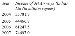
Source: Prowess (V. 3.1), Centre for Monitoring Indian Economy Pvt. Ltd, Mumbai, accessed September 2008, reproduced with permission.
The Indian aviation industry’s growth is vital in the light of continuous economic development. Increasing disposable incomes and the increasing number of Indians travelling overseas both for business and for leisure are some of the factors that have contributed to the growth of the Indian aviation industry. On the other side, increasing fuel prices, congestion at many metropolitan airports, shortage of skilled manpower, particularly pilots and engineers are some of the problems that it is facing.
- 1. Suppose the company wants to check the quality of inflight food. The quality control officer of the company has taken 63 randomly sampled packets of food and divided the quality in two categories: “good quality” (G) and “poor quality” (P). The results are given as below:
G,G,G,G,G,G,P,P,P,P,G,G,G,G,G,G,G,P,P,P,G,G,G, G,G,P,P,P,P,G,G,G,G,G,G,G,P,P,P,G,G,G,G,G,P,P,G,G,G,G,G,G,G,P,P,P,P,G,G,G,G,G,G
Use α = 0.05 to determine whether the samples are randomly selected.
- 2. Suppose the company has introduced new features to enhance customer satisfaction. After six months of the introduction of the new services, the company conducted a survey by administering questionnaires to two groups of travellers: “Executive class” and “Economy class.” The scores obtained from 13 randomly selected customers of “executive class” and 14 randomly selected customers of “economy class” are given in the table below:
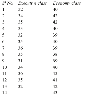
The company believes that the new services offered have attracted more executive class customers. Use the Mann–Whitney U test to determine whether the two populations differ in terms of customer satisfaction. Use α = 0.05.
- 3. Suppose the company wants to estimate the expenditure pattern of different customers based on four different occupations. The company has appointed a professional researcher who has obtained random samples from the customers from four different occupational backgrounds with respect to their expenditure (in thousand rupees) on air travel. The table below indicates the expenditure pattern. Use the Kruskal–Wallis test to determine whether there is a significant difference between customers’ occupational backgrounds in terms of their spending on travel. Use α = 0.05.
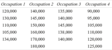
NOTES |
- 1. Prowess (V. 2.6), Centre for Monitoring Indian Economy Pvt. Ltd, Mumbai, accessed July 2007, reproduced with permission.
- 2. Prowess (V. 3.1), Centre for Monitoring Indian Economy Pvt. Ltd, Mumbai, accessed September 2008, reproduced with permission.
- 3. www.business-standard.com/india/storypage.php?autono = 333769, accessed September 2008.