37.1 VARIATIONS OF QUANTITATIVE STRATEGIES
At the heart of every equity market neutral strategy is the attempt to establish long positions in securities when their expected returns are relatively high and to establish short positions in securities when their expected returns are relatively low. Quantitative equity market neutral strategies can be divided based on underlying information (technical factors vs. fundamental factors) or trading frequencies.
37.1.1 Quantitative Strategies Focused on Technical Analysis
Quantitative equity market neutral strategies trade equities in a systematic fashion. Common techniques are based on sorting stocks given a particular indicator. The underlying indicator may be based purely on past prices and volume (i.e., technical analysis). An example would be the identification of a pairs trade between two stocks that have a high long-term correlation but recently experienced a sharp diversion in returns, widening the spread between the prices of the two stocks. A typical trading decision would be to establish a long position in the stock that had recently underperformed and a short position in the stock that had recently outperformed. The motivation for the trade would be the expectation that the stocks would converge to similar valuation levels based on their observed tendency to share similar returns and valuation levels. The trader would be speculating that the divergence in returns was temporary, perhaps based on the execution of a large order. A pairs trade is typically structured on a market neutral basis. Not only is the market beta offset, but industry and size factors are often neutralized in pairs trading.
The exact forms of technical analysis used to identify trades vary tremendously. However, the approaches are often distinguished by assuming either mean reversion or momentum (trending). Mean reversion is a tendency to return to typical historical relationships or levels, while momentum is a tendency of returns or valuation levels to persist in recently observed directions.
A popular statistical modeling approach is co-integration. Co-integration, as described in laymen's terms by Murray (1994), is analogous to the relationship between a drunken person and that person's dog, both walking aimlessly. Because the dog is on a leash, there is a limit to the distance between the person and the dog. Though both may appear to meander randomly and wildly over time, they move less wildly and widely as they continually adjust their positions closer to each other as they try to reunite. Thus, the two are co-integrated. The key to applying a co-integration approach is statistically identifying a relationship that persists.
Applying co-integration or a similar statistical approach to securities typically involves a daunting scale. For example, consider the possible combinations of securities in the S&P 500 index. The number of pairs is solved by “500 choose 2” or by thinking about it this way: given the matrix 500 × 500, exclude the diagonal (500), divide by 2, and take only one diagonal. So, [(500 × 500) – 500]/2 = 124,750 possible pairs. For each pair, the approach involves identifying the extent, if any, of the co-integration. A fund manager may establish potential patterns based on past data and then monitor the possible opportunities of each pair over time. Monitoring this number of co-integrated pairs over time may be a useful exercise to gauge the opportunity set for generic pairs trading. Obviously, one would have to account for many other issues, such as nuances of defining distance between pairs, transaction costs, market impact, short availability, and rebates. But as a simple exercise, such a barometer of the opportunity set may be useful.
Other techniques include decomposing the contents of a large variance-covariance matrix or correlation matrix into components that explain the main structure. Typically, this decomposition leads to statistically constructed orthogonal factors. For example, if one takes all the stocks in the S&P 500 and looks at the first principal component, chances are that it will look quite similar to the long-only market portfolio. That is, empirically, the first factor resembles the buy-and-hold S&P 500. The second principal component is more difficult to identify, but by construction, it is rendered orthogonal to the first component. Some statistical arbitrage funds (stat arb funds) attempt to model and trade higher-order components, or at least those that have some mean-reversion properties. That is, they will not trade the first principal component or the long-only market; they will try to model and trade higher-order factors. Once again, the bet is that ultimately, when things get stretched (when the drunken person and the dog are far away from each other), there will be a time when there is a convergence (the person and the dog will eventually move closer to each other). Measuring distances and timing are very important, and stat arb managers find taking a scientific approach useful in defining the needed terms.
Stat arb managers as a group are typically made up of doctorate-level scientists, mathematicians, and statisticians from leading academic institutions, all of whom have a strong background in analyzing large data sets. Common issues faced by these experts involve the most efficient clustering techniques, the newest machine-learning methods, and principal/independent component analysis. Generally, the goal becomes finding stable distributions or, if distributions are unstable, ways to detect this change of regimes so that positions correctly anticipate transitions to a new regime. With stable distributions, it is increasingly likely that the approach will eventually generate profits, much like the house at a casino will win in the long run if it sets up the payoff of the games correctly. Stat arb managers have the law of large numbers working in their favor if they are placing numerous bets over long periods of time on relationships that they are able to successfully identify and predict as being stable.
The most advanced techniques are often borrowed from other disciplines, such as econometrics and time-series analysis. Successful stat arb managers often have very little fundamental knowledge of the underlying stocks that they hold in their portfolios. These managers fall at one extreme end of the spectrum compared to long/short fundamental managers, who are more likely to have intimate knowledge of their companies.
37.1.2 Quantitative Strategies Based on Fundamental Factors
The underlying information driving trading decisions may be based on fundamental factors. Common fundamental indicators are book-to-market-value (B/M) ratio, earnings-to-price (E/P) ratio, cash-flow-to-price (CF/P) ratio, size, and so forth. The primary approach is to identify securities with abnormally high or low expected returns based on fundamental factors and an analysis of past return tendencies. For example, research may show that a particular combination of indicators has cross-sectionally differentiated average returns. A fund manager may assume that the fundamental factors can be used to predict relative expected returns, with long positions being established in those securities forecasted to offer higher expected returns, and short positions being established in those securities forecasted to offer lower expected returns. Some quantitative managers use a combination of technical and fundamental indicators in their trading models. One of the most frequently used model combinations is value plus momentum (discussed in a later section).
The underlying assumption of the use of fundamental factors to establish positions is stability in the relationship. Specifically, the fund manager is assuming that the past relationship between indicators and returns is likely to hold over time, such that relative future expected returns can be predicted. However, the risks are (1) that the observed relationship in the past was a random outcome with no predictive value, (2) that the observed relationship in the past has been corrected through increased informational efficiency or through fundamental changes in underlying economic relationships, and (3) that during periods of stress and other extreme conditions, the historically observed relationship unravels and reverses.
A distinction between a quantitative EMN strategy based on fundamental factors and the fundamental equity hedge funds discussed in Chapter 36 is the extent to which the analysis is based on extensive computational analysis of past returns and current prices. Fundamental equity hedge funds tend to perform extensive fundamental analysis on individual securities based on economic reasoning. Alternatively, quantitative analysts rely more on computerized analysis of large data sets for historical relationships between returns and fundamental factors, typically to predict short-term return differences. Fundamental analysts may screen data and organize data with computers, but their trading decisions are typically based on close examination of smaller data sets to project longer-term valuations.
37.1.3 Quantitative Strategies Differentiated by Trading Frequency
An important distinction between quantitative EMN funds is the trading frequency. The trading frequency is generally described as the typical length of time that positions are held (i.e., the holding period). Trading speed is calculated in terms of how fast one's model is able to take input information, create the signal, and then submit the orders into the markets for execution.
Exhibit 37.1 describes the spectrum of trading frequency among quantitative equity hedge funds. On the left end of the spectrum is high-frequency trading (HFT), in which trades are detected and executed in milliseconds and held possibly for only seconds. The challenge faced by most HFT approaches is generating greater speed than competitors in identifying and executing trades. The idea that drives each trade is typically rather simple; for example, one trading approach is a market-maker approach that identifies temporary price disequilibria presumably caused by large order executions. Another approach is to exploit slow security price responses to new information.
EXHIBIT 37.1 Competitive Advantage versus Trading Interval
Note: A millisecond is 1/1,000 of a second.
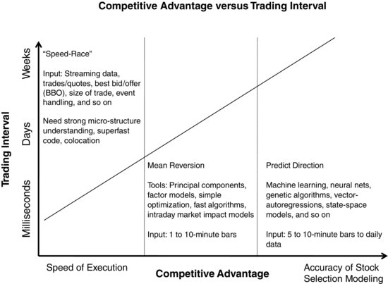
In the middle of Exhibit 37.1 are less rapid trading approaches that typically rely on mean reversion. These approaches require moderate speed and moderately advanced idea generation. On the right side of Exhibit 37.1 are the more directional approaches, which depend little on speed and most on accuracy of the economic modeling of future returns. These approaches are discussed further in a subsequent section.