
Chapter 6. The Cassandra Architecture
3.2 Architecture - fundamental concepts or properties of a system in its environment embodied in its elements, relationships, and in the principles of its design and evolution.
ISO/IEC/IEEE 42010
In this chapter, we examine several aspects of Cassandra’s architecture in order to understand how it does its job. We’ll explain the topology of a cluster, and how nodes interact in a peer-to-peer design to maintain the health of the cluster and exchange data, using techniques like gossip, anti-entropy, and hinted handoff. Looking inside the design of a node, we examine architecture techniques Cassandra uses to support reading, writing, and deleting data, and examine how these choices affect architectural considerations such as scalability, durability, availability, manageability, and more. We also discuss Cassandra’s adoption of a Staged Event-Driven Architecture, which acts as the platform for request delegation.
As we introduce these topics, we also provide references to where you can find their implementations in the Cassandra source code.
Data Centers and Racks
Cassandra is frequently used in systems spanning physically separate locations. Cassandra provides two levels of grouping that are used to describe the topology of a cluster: data center and rack. A rack is a logical set of nodes in close proximity to each other, perhaps on physical machines in a single rack of equipment. A data center is a logical set of racks, perhaps located in the same building and connected by reliable network. A sample topology with multiple data centers and racks is shown in Figure 6-1.
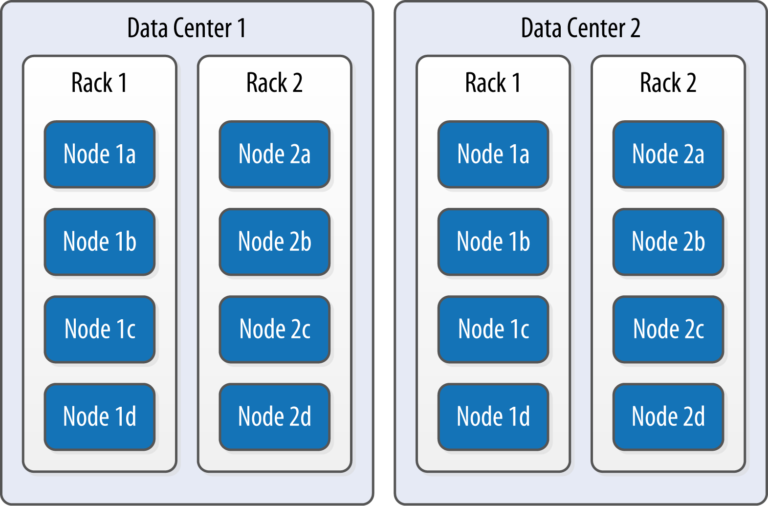
Figure 6-1. Topology of a sample cluster with data centers, racks, and nodes
Out of the box, Cassandra comes with a default configuration of a single data center ("DC1") containing a single rack ("RAC1"). We’ll learn in Chapter 7 how to build a larger cluster and define its topology.
Cassandra leverages the information you provide about your cluster’s topology to determine where to store data, and how to route queries efficiently. Cassandra tries to store copies of your data in multiple data centers to maximize availability and partition tolerance, while preferring to route queries to nodes in the local data center to maximize performance.
Gossip and Failure Detection
To support decentralization and partition tolerance, Cassandra uses a gossip protocol that allows each node to keep track of state information about the other nodes in the cluster. The gossiper runs every second on a timer.
Gossip protocols (sometimes called “epidemic protocols”) generally assume a faulty network, are commonly employed in very large, decentralized network systems, and are often used as an automatic mechanism for replication in distributed databases. They take their name from the concept of human gossip, a form of communication in which peers can choose with whom they want to exchange information.
The Origin of “Gossip Protocol”
The term “gossip protocol” was originally coined in 1987 by Alan Demers, a researcher at Xerox’s Palo Alto Research Center, who was studying ways to route information through unreliable networks.
The gossip protocol in Cassandra is primarily implemented by the org.apache.cassandra.gms.Gossiper class, which is responsible for managing gossip for the local node. When a server node is started, it registers itself with the gossiper to receive endpoint state information.
Because Cassandra gossip is used for failure detection, the Gossiper class maintains a list of nodes that are alive and dead.
Here is how the gossiper works:
-
Once per second, the gossiper will choose a random node in the cluster and initialize a gossip session with it. Each round of gossip requires three messages.
-
The gossip initiator sends its chosen friend a
GossipDigestSynMessage. -
When the friend receives this message, it returns a
GossipDigestAckMessage. -
When the initiator receives the
ackmessage from the friend, it sends the friend aGossipDigestAck2Messageto complete the round of gossip.
When the gossiper determines that another endpoint is dead, it “convicts” that endpoint by marking it as dead in its local list and logging that fact.
Cassandra has robust support for failure detection, as specified by a popular algorithm for distributed computing called Phi Accrual Failure Detection. This manner of failure detection originated at the Advanced Institute of Science and Technology in Japan in 2004.
Accrual failure detection is based on two primary ideas. The first general idea is that failure detection should be flexible, which is achieved by decoupling it from the application being monitored. The second and more novel idea challenges the notion of traditional failure detectors, which are implemented by simple “heartbeats” and decide whether a node is dead or not dead based on whether a heartbeat is received or not. But accrual failure detection decides that this approach is naive, and finds a place in between the extremes of dead and alive—a suspicion level.
Therefore, the failure monitoring system outputs a continuous level of “suspicion” regarding how confident it is that a node has failed. This is desirable because it can take into account fluctuations in the network environment. For example, just because one connection gets caught up doesn’t necessarily mean that the whole node is dead. So suspicion offers a more fluid and proactive indication of the weaker or stronger possibility of failure based on interpretation (the sampling of heartbeats), as opposed to a simple binary assessment.
Failure detection is implemented in Cassandra by the org.apache.cassandra.gms.FailureDetector class, which implements the org.apache.cassandra.gms.IFailureDetector interface. Together, they allow operations including:
Snitches
The job of a snitch is to determine relative host proximity for each node in a cluster, which is used to determine which nodes to read and write from. Snitches gather information about your network topology so that Cassandra can efficiently route requests. The snitch will figure out where nodes are in relation to other nodes.
As an example, let’s examine how the snitch participates in a read operation. When Cassandra performs a read, it must contact a number of replicas determined by the consistency level. In order to support the maximum speed for reads, Cassandra selects a single replica to query for the full object, and asks additional replicas for hash values in order to ensure the latest version of the requested data is returned. The role of the snitch is to help identify the replica that will return the fastest, and this is the replica which is queried for the full data.
The default snitch (the SimpleSnitch) is topology unaware; that is, it does not know about the racks and data centers in a cluster, which makes it unsuitable for multi-data center deployments. For this reason, Cassandra comes with several snitches for different cloud environments including Amazon EC2, Google Cloud, and Apache Cloudstack.
The snitches can be found in the package org.apache.cassandra.locator. Each snitch implements the IEndpointSnitch interface. We’ll learn how to select and configure an appropriate snitch for your environment in Chapter 7.
While Cassandra provides a pluggable way to statically describe your cluster’s topology, it also provides a feature called dynamic snitching that helps optimize the routing of reads and writes over time. Here’s how it works. Your selected snitch is wrapped with another snitch called the DynamicEndpointSnitch. The dynamic snitch gets its basic understanding of the topology from the selected snitch. It then monitors the performance of requests to the other nodes, even keeping track of things like which nodes are performing compaction. The performance data is used to select the best replica for each query. This enables Cassandra to avoid routing requests to replicas that are performing poorly.
The dynamic snitching implementation uses a modified version of the Phi failure detection mechanism used by gossip. The “badness threshold” is a configurable parameter that determines how much worse a preferred node must perform than the best-performing node in order to lose its preferential status. The scores of each node are reset periodically in order to allow a poorly performing node to demonstrate that it has recovered and reclaim its preferred status.
Rings and Tokens
So far we’ve been focusing on how Cassandra keeps track of the physical layout of nodes in a cluster. Let’s shift gears and look at how Cassandra distributes data across these nodes.
Cassandra represents the data managed by a cluster as a ring. Each node in the ring is assigned one or more ranges of data described by a token, which determines its position in the ring. A token is a 64-bit integer ID used to identify each partition. This gives a possible range for tokens from –263 to 263–1.
A node claims ownership of the range of values less than or equal to each token and greater than the token of the previous node. The node with lowest token owns the range less than or equal to its token and the range greater than the highest token, which is also known as the “wrapping range.” In this way, the tokens specify a complete ring. Figure 6-2 shows a notional ring layout including the nodes in a single data center. This particular arrangement is structured such that consecutive token ranges are spread across nodes in different racks.
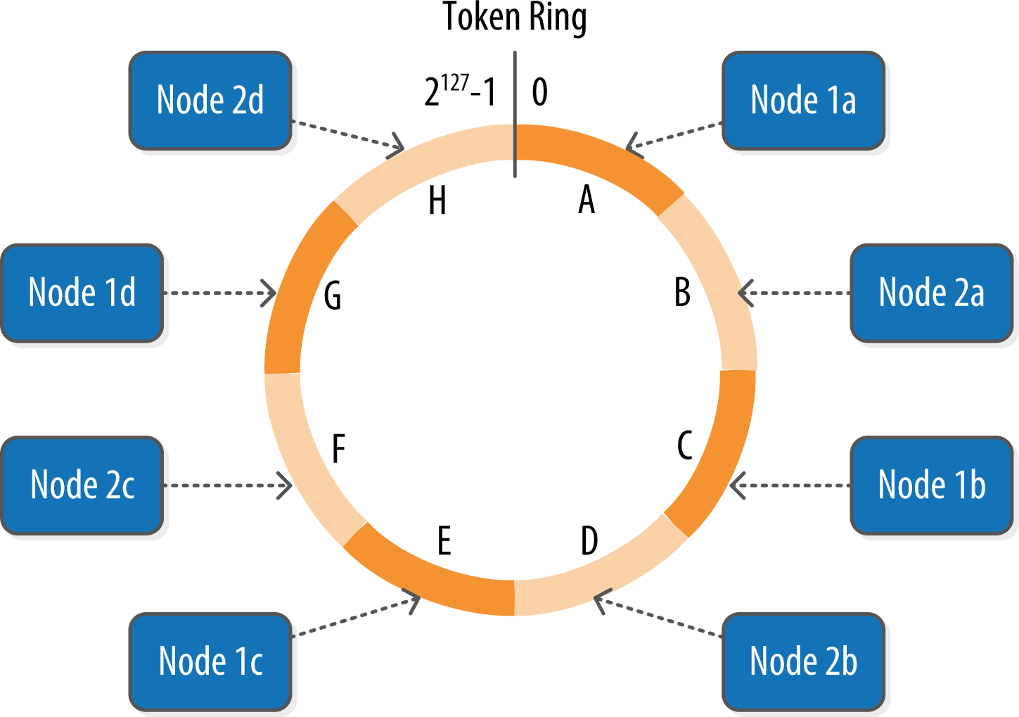
Figure 6-2. Example ring arrangement of nodes in a data center
Data is assigned to nodes by using a hash function to calculate a token for the partition key. This partition key token is compared to the token values for the various nodes to identify the range, and therefore the node, that owns the data.
Token ranges are represented by the org.apache.cassandra.dht.Range class.
Virtual Nodes
Early versions of Cassandra assigned a single token to each node, in a fairly static manner, requiring you to calculate tokens for each node. Although there are tools available to calculate tokens based on a given number of nodes, it was still a manual process to configure the initial_token property for each node in the cassandra.yaml file. This also made adding or replacing a node an expensive operation, as rebalancing the cluster required moving a lot of data.
Cassandra’s 1.2 release introduced the concept of virtual nodes, also called vnodes for short. Instead of assigning a single token to a node, the token range is broken up into multiple smaller ranges. Each physical node is then assigned multiple tokens. By default, each node will be assigned 256 of these tokens, meaning that it contains 256 virtual nodes. Virtual nodes have been enabled by default since 2.0.
Vnodes make it easier to maintain a cluster containing heterogeneous machines. For nodes in your cluster that have more computing resources available to them, you can increase the number of vnodes by setting the num_tokens property in the cassandra.yaml file. Conversely, you might set num_tokens lower to decrease the number of vnodes for less capable machines.
Cassandra automatically handles the calculation of token ranges for each node in the cluster in proportion to their num_tokens value. Token assignments for vnodes are calculated by the org.apache.cassandra.dht.tokenallocator.ReplicationAwareTokenAllocator class.
A further advantage of virtual nodes is that they speed up some of the more heavyweight Cassandra operations such as bootstrapping a new node, decommissioning a node, and repairing a node. This is because the load associated with operations on multiple smaller ranges is spread more evenly across the nodes in the cluster.
Partitioners
A partitioner determines how data is distributed across the nodes in the cluster. As we learned in Chapter 5, Cassandra stores data in wide rows, or “partitions.” Each row has a partition key that is used to identify the partition. A partitioner, then, is a hash function for computing the token of a partition key. Each row of data is distributed within the ring according to the value of the partition key token.
Cassandra provides several different partitioners in the org.apache.cassandra.dht package (DHT stands for “distributed hash table”). The Murmur3Partitioner was added in 1.2 and has been the default partitioner since then; it is an efficient Java implementation on the murmur algorithm developed by Austin Appleby. It generates 64-bit hashes. The previous default was the RandomPartitioner.
Because of Cassandra’s generally pluggable design, you can also create your own partitioner by implementing the org.apache.cassandra.dht.IPartitioner class and placing it on Cassandra’s classpath.
Replication Strategies
A node serves as a replica for different ranges of data. If one node goes down, other replicas can respond to queries for that range of data. Cassandra replicates data across nodes in a manner transparent to the user, and the replication factor is the number of nodes in your cluster that will receive copies (replicas) of the same data. If your replication factor is 3, then three nodes in the ring will have copies of each row.
The first replica will always be the node that claims the range in which the token falls, but the remainder of the replicas are placed according to the replication strategy (sometimes also referred to as the replica placement strategy).
For determining replica placement, Cassandra implements the Gang of Four Strategy pattern, which is outlined in the common abstract class org.apache.cassandra.locator.AbstractReplicationStrategy, allowing different implementations of an algorithm (different strategies for accomplishing the same work). Each algorithm implementation is encapsulated inside a single class that extends the AbstractReplicationStrategy.
Out of the box, Cassandra provides two primary implementations of this interface (extensions of the abstract class): SimpleStrategy and NetworkTopologyStrategy. The SimpleStrategy places replicas at consecutive nodes around the ring, starting with the node indicated by the partitioner. The NetworkTopologyStrategy allows you to specify a different replication factor for each data center. Within a data center, it allocates replicas to different racks in order to maximize availability.
Legacy Replication Strategies
A third strategy, OldNetworkTopologyStrategy, is provided for backward compatibility. It was previously known as the RackAwareStrategy, while the SimpleStrategy was previously known as the RackUnawareStrategy. NetworkTopologyStrategy was previously known as DataCenterShardStrategy. These changes were effective in the 0.7 release.
The strategy is set independently for each keyspace and is a required option to create a keyspace, as we saw in Chapter 5.
Consistency Levels
In Chapter 2, we discussed Brewer’s CAP theorem, in which consistency, availability, and partition tolerance are traded off against one another. Cassandra provides tuneable consistency levels that allow you to make these trade-offs at a fine-grained level. You specify a consistency level on each read or write query that indicates how much consistency you require. A higher consistency level means that more nodes need to respond to a read or write query, giving you more assurance that the values present on each replica are the same.
For read queries, the consistency level specifies how many replica nodes must respond to a read request before returning the data. For write operations, the consistency level specifies how many replica nodes must respond for the write to be reported as successful to the client. Because Cassandra is eventually consistent, updates to other replica nodes may continue in the background.
The available consistency levels include ONE, TWO, and THREE, each of which specify an absolute number of replica nodes that must respond to a request. The QUORUM consistency level requires a response from a majority of the replica nodes (sometimes expressed as “replication factor / 2 + 1”). The ALL consistency level requires a response from all of the replicas. We’ll examine these consistency levels and others in more detail in Chapter 9.
For both reads and writes, the consistency levels of ANY, ONE, TWO, and THREE are considered weak, whereas QUORUM and ALL are considered strong. Consistency is tuneable in Cassandra because clients can specify the desired consistency level on both reads and writes. There is an equation that is popularly used to represent the way to achieve strong consistency in Cassandra: R + W > N = strong consistency. In this equation, R, W, and N are the read replica count, the write replica count, and the replication factor, respectively; all client reads will see the most recent write in this scenario, and you will have strong consistency.
Distinguishing Consistency Levels and Replication Factors
If you’re new to Cassandra, the replication factor can sometimes be confused with the consistency level. The replication factor is set per keyspace. The consistency level is specified per query, by the client. The replication factor indicates how many nodes you want to use to store a value during each write operation. The consistency level specifies how many nodes the client has decided must respond in order to feel confident of a successful read or write operation. The confusion arises because the consistency level is based on the replication factor, not on the number of nodes in the system.
Queries and Coordinator Nodes
Let’s bring these concepts together to discuss how Cassandra nodes interact to support reads and writes from client applications. Figure 6-3 shows the typical path of interactions with Cassandra.
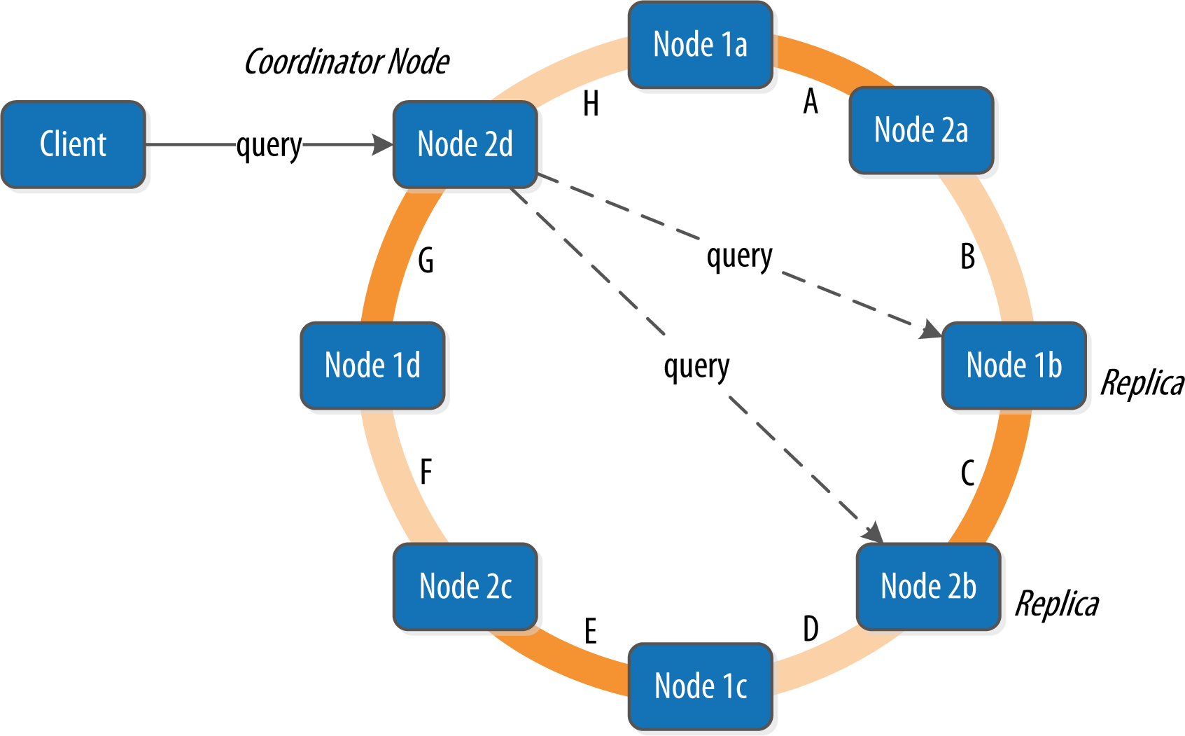
Figure 6-3. Clients, coordinator nodes, and replicas
A client may connect to any node in the cluster to initiate a read or write query. This node is known as the coordinator node. The coordinator identifies which nodes are replicas for the data that is being written or read and forwards the queries to them.
For a write, the coordinator node contacts all replicas, as determined by the consistency level and replication factor, and considers the write successful when a number of replicas commensurate with the consistency level acknowledge the write.
For a read, the coordinator contacts enough replicas to ensure the required consistency level is met, and returns the data to the client.
These, of course, are the “happy path” descriptions of how Cassandra works. We’ll soon discuss some of Cassandra’s high availability mechanisms, including hinted handoff.
Memtables, SSTables, and Commit Logs
Now let’s take a look at some of Cassandra’s internal data structures and files, summarized in Figure 6-4. Cassandra stores data both in memory and on disk to provide both high performance and durability. In this section, we’ll focus on Cassandra’s use of constructs called memtables, SSTables, and commit logs to support the writing and reading of data from tables.

Figure 6-4. Internal data structures and files of a Cassandra node
When you perform a write operation, it’s immediately written to a commit log. The commit log is a crash-recovery mechanism that supports Cassandra’s durability goals. A write will not count as successful until it’s written to the commit log, to ensure that if a write operation does not make it to the in-memory store (the memtable, discussed in a moment), it will still be possible to recover the data. If you shut down the database or it crashes unexpectedly, the commit log can ensure that data is not lost. That’s because the next time you start the node, the commit log gets replayed. In fact, that’s the only time the commit log is read; clients never read from it.
After it’s written to the commit log, the value is written to a memory-resident data structure called the memtable. Each memtable contains data for a specific table. In early implementations of Cassandra, memtables were stored on the JVM heap, but improvements starting with the 2.1 release have moved the majority of memtable data to native memory. This makes Cassandra less susceptible to fluctuations in performance due to Java garbage collection.
When the number of objects stored in the memtable reaches a threshold, the contents of the memtable are flushed to disk in a file called an SSTable. A new memtable is then created. This flushing is a non-blocking operation; multiple memtables may exist for a single table, one current and the rest waiting to be flushed. They typically should not have to wait very long, as the node should flush them very quickly unless it is overloaded.
Each commit log maintains an internal bit flag to indicate whether it needs flushing. When a write operation is first received, it is written to the commit log and its bit flag is set to 1. There is only one bit flag per table, because only one commit log is ever being written to across the entire server. All writes to all tables will go into the same commit log, so the bit flag indicates whether a particular commit log contains anything that hasn’t been flushed for a particular table. Once the memtable has been properly flushed to disk, the corresponding commit log’s bit flag is set to 0, indicating that the commit log no longer has to maintain that data for durability purposes. Like regular logfiles, commit logs have a configurable rollover threshold, and once this file size threshold is reached, the log will roll over, carrying with it any extant dirty bit flags.
The SSTable is a concept borrowed from Google’s Bigtable. Once a memtable is flushed to disk as an SSTable, it is immutable and cannot be changed by the application. Despite the fact that SSTables are compacted, this compaction changes only their on-disk representation; it essentially performs the “merge” step of a mergesort into new files and removes the old files on success.
Why Are They Called “SSTables”?
The idea that “SSTable” is a compaction of “Sorted String Table” is somewhat inaccurate for Cassandra, because the data is not stored as strings on disk.
Since the 1.0 release, Cassandra has supported the compression of SSTables in order to maximize use of the available storage. This compression is configurable per table. Each SSTable also has an associated Bloom filter, which is used as an additional performance enhancer (see “Bloom Filters”).
All writes are sequential, which is the primary reason that writes perform so well in Cassandra. No reads or seeks of any kind are required for writing a value to Cassandra because all writes are append operations. This makes one key limitation on performance the speed of your disk. Compaction is intended to amortize the reorganization of data, but it uses sequential I/O to do so. So the performance benefit is gained by splitting; the write operation is just an immediate append, and then compaction helps to organize for better future read performance. If Cassandra naively inserted values where they ultimately belonged, writing clients would pay for seeks up front.
On reads, Cassandra will read both SSTables and memtables to find data values, as the memtable may contain values that have not yet been flushed to disk. Memtables are implemented by the org.apache.cassandra.db.Memtable class.
Caching
As we saw in Figure 6-4, Cassandra provides three forms of caching:
- The key cache stores a map of partition keys to row index entries, facilitating faster read access into SSTables stored on disk. The key cache is stored on the JVM heap.
- The row cache caches entire rows and can greatly speed up read access for frequently accessed rows, at the cost of more memory usage. The row cache is stored in off-heap memory.
- The counter cache was added in the 2.1 release to improve counter performance by reducing lock contention for the most frequently accessed counters.
By default, key and counter caching are enabled, while row caching is disabled, as it requires more memory. Cassandra saves its caches to disk periodically in order to warm them up more quickly on a node restart. We’ll investigate how to tune these caches in Chapter 12.
Hinted Handoff
Consider the following scenario: a write request is sent to Cassandra, but a replica node where the write properly belongs is not available due to network partition, hardware failure, or some other reason. In order to ensure general availability of the ring in such a situation, Cassandra implements a feature called hinted handoff. You might think of a hint as a little Post-it note that contains the information from the write request. If the replica node where the write belongs has failed, the coordinator will create a hint, which is a small reminder that says, “I have the write information that is intended for node B. I’m going to hang onto this write, and I’ll notice when node B comes back online; when it does, I’ll send it the write request.” That is, once it detects via gossip that node B is back online, node A will “hand off” to node B the “hint” regarding the write. Cassandra holds a separate hint for each partition that is to be written.
This allows Cassandra to be always available for writes, and generally enables a cluster to sustain the same write load even when some of the nodes are down. It also reduces the time that a failed node will be inconsistent after it does come back online.
In general, hints do not count as writes for the purposes of consistency level. The exception is the consistency level ANY, which was added in 0.6. This consistency level means that a hinted handoff alone will count as sufficient toward the success of a write operation. That is, even if only a hint was able to be recorded, the write still counts as successful. Note that the write is considered durable, but the data may not be readable until the hint is delivered to the target replica.
Hinted Handoff and Guaranteed Delivery
Hinted handoff is used in Amazon’s Dynamo and is familiar to those who are aware of the concept of guaranteed delivery in messaging systems such as the Java Message Service (JMS). In a durable guaranteed-delivery JMS queue, if a message cannot be delivered to a receiver, JMS will wait for a given interval and then resend the request until the message is received.
There is a practical problem with hinted handoffs (and guaranteed delivery approaches, for that matter): if a node is offline for some time, the hints can build up considerably on other nodes. Then, when the other nodes notice that the failed node has come back online, they tend to flood that node with requests, just at the moment it is most vulnerable (when it is struggling to come back into play after a failure). To address this problem, Cassandra limits the storage of hints to a configurable time window. It is also possible to disable hinted handoff entirely.
As its name suggests, org.apache.cassandra.db.HintedHandOffManager is the class that manages hinted handoffs internally.
Although hinted handoff helps increase Cassandra’s availability, it does not fully replace the need for manual repair to ensure consistency.
Lightweight Transactions and Paxos
As we discussed in Chapter 2, Cassandra provides tuneable consistency, including the ability to achieve strong consistency by specifying sufficiently high consistency levels. However, strong consistency is not enough to prevent race conditions in cases where clients need to read, then write data.
To help explain this with an example, let’s revisit our my_keyspace.user table from Chapter 5. Imagine we are building a client that wants to manage user records as part of an account management application. In creating a new user account, we’d like to make sure that the user record doesn’t already exist, lest we unintentionally overwrite existing user data. So we do a read to see if the record exists first, and then only perform the create if the record doesn’t exist.
The behavior we’re looking for is called linearizable consistency, meaning that we’d like to guarantee that no other client can come in between our read and write queries with their own modification. Since the 2.0 release, Cassandra supports a lightweight transaction (or “LWT”) mechanism that provides linearizable consistency.
Cassandra’s LWT implementation is based on Paxos. Paxos is a consensus algorithm that allows distributed peer nodes to agree on a proposal, without requiring a master to coordinate a transaction. Paxos and other consensus algorithms emerged as alternatives to traditional two-phase commit based approaches to distributed transactions (reference the note on Two-Phase Commit in The Problem with Two-Phase Commit).
The basic Paxos algorithm consists of two stages: prepare/promise, and propose/accept. To modify data, a coordinator node can propose a new value to the replica nodes, taking on the role of leader. Other nodes may act as leaders simultaneously for other modifications. Each replica node checks the proposal, and if the proposal is the latest it has seen, it promises to not accept proposals associated with any prior proposals. Each replica node also returns the last proposal it received that is still in progress. If the proposal is approved by a majority of replicas, the leader commits the proposal, but with the caveat that it must first commit any in-progress proposals that preceded its own proposal.
The Cassandra implementation extends the basic Paxos algorithm in order to support the desired read-before-write semantics (also known as “check-and-set”), and to allow the state to be reset between transactions. It does this by inserting two additional phases into the algorithm, so that it works as follows:
- Prepare/Promise
- Read/Results
- Propose/Accept
- Commit/Ack
Thus, a successful transaction requires four round-trips between the coordinator node and replicas. This is more expensive than a regular write, which is why you should think carefully about your use case before using LWTs.
More on Paxos
Several papers have been written about the Paxos protocol. One of the best explanations available is Leslie Lamport’s “Paxos Made Simple”.
Cassandra’s lightweight transactions are limited to a single partition. Internally, Cassandra stores a Paxos state for each partition. This ensures that transactions on different partitions cannot interfere with each other.
You can find Cassandra’s implementation of the Paxos algorithm in the package org.apache.cassandra.service.paxos. These classes are leveraged by the StorageService, which we will learn about soon.
Tombstones
In the relational world, you might be accustomed to the idea of a “soft delete.” Instead of actually executing a delete SQL statement, the application will issue an update statement that changes a value in a column called something like “deleted.” Programmers sometimes do this to support audit trails, for example.
There’s a similar concept in Cassandra called a tombstone. This is how all deletes work and is therefore automatically handled for you. When you execute a delete operation, the data is not immediately deleted. Instead, it’s treated as an update operation that places a tombstone on the value. A tombstone is a deletion marker that is required to suppress older data in SSTables until compaction can run.
There’s a related setting called Garbage Collection Grace Seconds. This is the amount of time that the server will wait to garbage-collect a tombstone. By default, it’s set to 864,000 seconds, the equivalent of 10 days. Cassandra keeps track of tombstone age, and once a tombstone is older than GCGraceSeconds, it will be garbage-collected. The purpose of this delay is to give a node that is unavailable time to recover; if a node is down longer than this value, then it is treated as failed and replaced.
Bloom Filters
Bloom filters are used to boost the performance of reads. They are named for their inventor, Burton Bloom. Bloom filters are very fast, non-deterministic algorithms for testing whether an element is a member of a set. They are non-deterministic because it is possible to get a false-positive read from a Bloom filter, but not a false-negative. Bloom filters work by mapping the values in a data set into a bit array and condensing a larger data set into a digest string using a hash function. The digest, by definition, uses a much smaller amount of memory than the original data would. The filters are stored in memory and are used to improve performance by reducing the need for disk access on key lookups. Disk access is typically much slower than memory access. So, in a way, a Bloom filter is a special kind of cache. When a query is performed, the Bloom filter is checked first before accessing disk. Because false-negatives are not possible, if the filter indicates that the element does not exist in the set, it certainly doesn’t; but if the filter thinks that the element is in the set, the disk is accessed to make sure.
Bloom filters are implemented by the org.apache.cassandra.utils.BloomFilter class. Cassandra provides the ability to increase Bloom filter accuracy (reducing the number of false positives) by increasing the filter size, at the cost of more memory. This false positive chance is tuneable per table.
Compaction
As we already discussed, SSTables are immutable, which helps Cassandra achieve such high write speeds. However, periodic compaction of these SSTables is important in order to support fast read performance and clean out stale data values. A compaction operation in Cassandra is performed in order to merge SSTables. During compaction, the data in SSTables is merged: the keys are merged, columns are combined, tombstones are discarded, and a new index is created.
Compaction is the process of freeing up space by merging large accumulated datafiles. This is roughly analogous to rebuilding a table in the relational world. But the primary difference in Cassandra is that it is intended as a transparent operation that is amortized across the life of the server.
On compaction, the merged data is sorted, a new index is created over the sorted data, and the freshly merged, sorted, and indexed data is written to a single new SSTable (each SSTable consists of multiple files including: Data, Index, and Filter). This process is managed by the class org.apache.cassandra.db.compaction.CompactionManager.
Another important function of compaction is to improve performance by reducing the number of required seeks. There are a bounded number of SSTables to inspect to find the column data for a given key. If a key is frequently mutated, it’s very likely that the mutations will all end up in flushed SSTables. Compacting them prevents the database from having to perform a seek to pull the data from each SSTable in order to locate the current value of each column requested in a read request.
When compaction is performed, there is a temporary spike in disk I/O and the size of data on disk while old SSTables are read and new SSTables are being written.
Cassandra supports multiple algorithms for compaction via the strategy pattern. The compaction strategy is an option that is set for each table. The compaction strategy extends the AbstractCompactionStrategy class. The available strategies include:
SizeTieredCompactionStrategy(STCS) is the default compaction strategy and is recommended for write-intensive tablesLeveledCompactionStrategy(LCS) is recommended for read-intensive tablesDateTieredCompactionStrategy(DTCS), which is intended for time series or otherwise date-based data.
We’ll revisit these strategies in Chapter 12 to discuss selecting the best strategy for each table.
One interesting feature of compaction relates to its intersection with incremental repair. A feature called anticompaction was added in 2.1. As the name implies, anticompaction is somewhat of an opposite operation to regular compaction in that the result is the division of an SSTable into two SSTables, one containing repaired data, and the other containing unrepaired data.
The trade-off is that more complexity is introduced into the compaction strategies, which must handle repaired and unrepaired SSTables separately so that they are not merged together.
What About Major Compaction?
Users with prior experience may recall that Cassandra exposes an administrative operation called major compaction (also known as full compaction) that consolidates multiple SSTables into a single SSTable. While this feature is still available, the utility of performing a major compaction has been greatly reduced over time. In fact, usage is actually discouraged in production environments, as it tends to limit Cassandra’s ability to remove stale data. We’ll learn more about this and other administrative operations on SSTables available via nodetool in Chapter 11.
Anti-Entropy, Repair, and Merkle Trees
Cassandra uses an anti-entropy protocol, which is a type of gossip protocol for repairing replicated data. Anti-entropy protocols work by comparing replicas of data and reconciling differences observed between the replicas. Anti-entropy is used in Amazon’s Dynamo, and Cassandra’s implementation is modeled on that (see Section 4.7 of the Dynamo paper).
Anti-Entropy in Cassandra
In Cassandra, the term anti-entropy is often used in two slightly different contexts, with meanings that have some overlap:
- The term is often used as a shorthand for the replica synchronization mechanism for ensuring that data on different nodes is updated to the newest version.
- At other times, Cassandra is described as having an anti-entropy capability that includes replica synchronization as well as hinted handoff, which is a write-time anti-entropy mechanism we read about in “Hinted Handoff”.
Replica synchronization is supported via two different modes known as read repair and anti-entropy repair. Read repair refers to the synchronization of replicas as data is read. Cassandra reads data from multiple replicas in order to achieve the requested consistency level, and detects if any replicas have out of date values. If an insufficient number of nodes have the latest value, a read repair is performed immediately to update the out of date replicas. Otherwise, the repairs can be performed in the background after the read returns. This design is observed by Cassandra as well as by straight key/value stores such as Project Voldemort and Riak.
Anti-entropy repair (sometimes called manual repair) is a manually initiated operation performed on nodes as part of a regular maintenance process. This type of repair is executed by using a tool called nodetool, as we’ll learn about in Chapter 11. Running nodetool repair causes Cassandra to execute a major compaction (see “Compaction”). During a major compaction, the server initiates a TreeRequest/TreeReponse conversation to exchange Merkle trees with neighboring nodes. The Merkle tree is a hash representing the data in that table. If the trees from the different nodes don’t match, they have to be reconciled (or “repaired”) to determine the latest data values they should all be set to. This tree comparison validation is the responsibility of the org.apache.cassandra.service.AbstractReadExecutor class.
Both Cassandra and Dynamo use Merkle trees for anti-entropy, but their implementations are a little different. In Cassandra, each table has its own Merkle tree; the tree is created as a snapshot during a major compaction, and is kept only as long as is required to send it to the neighboring nodes on the ring. The advantage of this implementation is that it reduces network I/O.
Staged Event-Driven Architecture (SEDA)
Cassandra’s design was influenced by Staged Event-Driven Architecture (SEDA). SEDA is a general architecture for highly concurrent Internet services, originally proposed in a 2001 paper called “SEDA: An Architecture for Well-Conditioned, Scalable Internet Services” by Matt Welsh, David Culler, and Eric Brewer (who you might recall from our discussion of the CAP theorem). You can read the original SEDA paper at http://www.eecs.harvard.edu/~mdw/proj/seda.
In a typical application, a single unit of work is often performed within the confines of a single thread. A write operation, for example, will start and end within the same thread. Cassandra, however, is different: its concurrency model is based on SEDA, so a single operation may start with one thread, which then hands off the work to another thread, which may hand it off to other threads. But it’s not up to the current thread to hand off the work to another thread. Instead, work is subdivided into what are called stages, and the thread pool (really, a java.util.concurrent.ExecutorService) associated with the stage determines execution.
A stage is a basic unit of work, and a single operation may internally state-transition from one stage to the next. Because each stage can be handled by a different thread pool, Cassandra experiences a massive performance improvement. This design also means that Cassandra is better able to manage its own resources internally because different operations might require disk I/O, or they might be CPU-bound, or they might be network operations, and so on, so the pools can manage their work according to the availability of these resources.
A stage consists of an incoming event queue, an event handler, and an associated thread pool. Stages are managed by a controller that determines scheduling and thread allocation; Cassandra implements this kind of concurrency model using the thread pool java.util.concurrent.ExecutorService. To see specifically how this works, check out the org.apache.cassandra.concurrent.StageManager class. The following operations are represented as stages in Cassandra, including many of the concepts we’ve discussed in this chapter:
- Read (local reads)
- Mutation (local writes)
- Gossip
- Request/response (interactions with other nodes)
- Anti-entropy (
nodetoolrepair) - Read repair
- Migration (making schema changes)
- Hinted handoff
You can observe the thread pools associated with each of these stages by using the nodetool tpstats command, which we’ll learn about in Chapter 10.
A few additional operations are also implemented as stages, such as operations on memtables including flushing data out to SSTables and freeing memory. The stages implement the IVerbHandler interface to support the functionality for a given verb. Because the idea of mutation is represented as a stage, it can play a role in both insert and delete operations.
A Pragmatic Approach to SEDA
Over time, developers of Cassandra and other technologies based on the SEDA architecture article have encountered performance issues due to the inefficiencies of requiring separate thread pools for each stage and event queues between each stage, even for short-lived stages. These challenges were acknowledged by Matt Welsh in the follow-up blog post “A Retrospective on SEDA”.
Over time, Cassandra’s developers have relaxed the strict SEDA conventions, collapsing some stages into the same thread pool to improve throughput. However, the basic principles of separating work into stages and using queues and thread pools to manage these stages are still in evidence in the code.
Managers and Services
There is a set of classes that form Cassandra’s basic internal control mechanisms. We’ve encountered a few of them already in this chapter, including the HintedHandOffManager, the CompactionManager, and the StageManager. We’ll present a brief overview of a few other classes here so that you can become familiar with some of the more important ones. Many of these expose MBeans via the Java Management Extension (JMX) in order to report status and metrics, and in some cases to allow configuration and control of their activities. We’ll learn more about interacting with these MBeans in Chapter 10.
Cassandra Daemon
The org.apache.cassandra.service.CassandraDaemon interface represents the life cycle of the Cassandra service running on a single node. It includes the typical life cycle operations that you might expect: start, stop, activate, deactivate, and destroy.
You can also create an in-memory Cassandra instance programmatically by using the class org.apache.cassandra.service.EmbeddedCassandraService. Creating an embedded instance can be useful for unit testing programs using Cassandra.
Storage Engine
Cassandra’s core data storage functionality is commonly referred to as the storage engine, which consists primarily of classes in the org.apache.cassandra.db package. The main entry point is the ColumnFamilyStore class, which manages all aspects of table storage, including commit logs, memtables, SSTables, and indexes.
Major Changes to the Storage Engine
The storage engine was largely rewritten for the 3.0 release to bring Cassandra’s in-memory and on-disk representations of data in alignment with the CQL. An excellent summary of the changes is provided in the CASSANDRA-8099 JIRA issue.
The storage engine rewrite was a precursor for many other changes, most importantly, support for materialized views, which was implemented under CASSANDRA-6477. These two JIRA issues make for interesting reading if you want to better understand the changes required “under the hood” to enable these powerful new features.
Storage Service
Cassandra wraps the storage engine with a service represented by the org.apache.cassandra.service.StorageService class. The storage service contains the node’s token, which is a marker indicating the range of data that the node is responsible for.
The server starts up with a call to the initServer method of this class, upon which the server registers the SEDA verb handlers, makes some determinations about its state (such as whether it was bootstrapped or not, and what its partitioner is), and registers an MBean with the JMX server.
Storage Proxy
The org.apache.cassandra.service.StorageProxy sits in front of the StorageService to handle the work of responding to client requests. It coordinates with other nodes to store and retrieve data, including storage of hints when needed. The StorageProxy also helps manage lightweight transaction processing.
Direct Invocation of the Storage Proxy
Although it is possible to invoke the StorageProxy programmatically, as an in-memory instance, note that this is not considered an officially supported API for Cassandra and therefore has undergone changes between releases.
Messaging Service
The purpose of org.apache.cassandra.net.MessagingService is to create socket listeners for message exchange; inbound and outbound messages from this node come through this service. The MessagingService.listen method creates a thread. Each incoming connection then dips into the ExecutorService thread pool using org.apache.cassandra.net.IncomingTcpConnection (a class that extends Thread) to deserialize the message. The message is validated, and then routed to the appropriate handler.
Because the MessagingService also makes heavy use of stages and the pool it maintains is wrapped with an MBean, you can find out a lot about how this service is working (whether reads are getting backed up and so forth) through JMX.
Stream Manager
Streaming is Cassandra’s optimized way of sending sections of SSTable files from one node to another via a persistent TCP connection; all other communication between nodes occurs via serialized messages. The org.apache.cassandra.streaming.StreamManager handles these streaming messages, including connection management, message compression, progress tracking, and statistics.
CQL Native Transport Server
The CQL Native Protocol is the binary protocol used by clients to communicate with Cassandra. The org.apache.cassandra.transport package contains the classes that implement this protocol, including the Server. This native transport server manages client connections and routes incoming requests, delegating the work of performing queries to the StorageProxy.
There are several other classes that manage key features of Cassandra. Here are a few to investigate if you’re interested:
| Key feature | Class |
|---|---|
| Repair | org.apache.cassandra.service.ActiveRepairService |
| Caching | org.apache.cassandra.service.CachingService |
| Migration | org.apache.cassandra.service.MigrationManager |
| Materialized views | org.apache.cassandra.db.view.MaterializedViewManager |
| Secondary indexes | org.apache.cassandra.db.index.SecondaryIndexManager |
| Authorization | org.apache.cassandra.auth.CassandraRoleManager |
System Keyspaces
In true “dogfooding” style, Cassandra makes use of its own storage to keep track of metadata about the cluster and local node. This is similar to the way in which Microsoft SQL Server maintains the meta-databases master and tempdb. The master is used to keep information about disk space, usage, system settings, and general server installation notes; the tempdb is used as a workspace to store intermediate results and perform general tasks. The Oracle database always has a tablespace called SYSTEM, used for similar purposes. The Cassandra system keyspaces are used much like these.
Let’s go back to cqlsh to have a quick peek at the tables in Cassandra’s system keyspace:
cqlsh> DESCRIBE TABLES;

Keyspace system_traces
----------------------
events sessions

Keyspace system_schema
----------------------
materialized_views  functions  aggregates  types            columns
tables              triggers   keyspaces   dropped_columns

Keyspace system_auth
--------------------
resource_role_permissons_index  role_permissions  role_members
roles

Keyspace system
---------------
available_ranges                       sstable_activity    local
range_xfers                            peer_events         hints
materialized_views_builds_in_progress  paxos
"IndexInfo"                            batchlog
peers                                  size_estimates
built_materialized_views               compaction_history

Keyspace system_distributed
---------------------------
repair_history  parent_repair_history
Seeing Different System Keyspaces?
If you’re using a version of Cassandra prior to 2.2, you may not see some of these keyspaces listed. While the basic system keyspace has been around since the beginning, the system_traces keyspace was added in 1.2 to support request tracing. The system_auth and system_distributed keyspaces were added in 2.2 to support role-based access control (RBAC) and persistence of repair data, respectively. Finally, tables related to schema definition were migrated from system to the system_schema keyspace in 3.0.
Looking over these tables, we see that many of them are related to the concepts discussed in this chapter:
- Information about the structure of the cluster communicated via gossip is stored in
system.localandsystem.peers. These tables hold information about the local node and other nodes in the cluster including IP addresses, locations by data center and rack, CQL, and protocol versions. - The
system.range_xfersandsystem.available_rangestrack token ranges managed by each node and any ranges needing allocation. - The
system_schema.keyspaces,system_schema.tables, andsystem_schema.columnsstore the definitions of the keyspaces, tables, and indexes defined for the cluster. - The construction of materialized views is tracked in the
system.materialized_views_builds_in_progressandsystem.built_materialized_viewstables, resulting in the views available insystem_schema.materialized_views. - User-provided extensions such as
system_schema.typesfor user-defined types,system_schema.triggersfor triggers configured per table,system_schema.functionsfor user-defined functions, andsystem_schema.aggregatesfor user-defined aggregates. - The
system.paxostable stores the status of transactions in progress, while thesystem.batchlogtable stores the status of atomic batches. - The
system.size_estimatesstores the estimated number of partitions per table, which is used for Hadoop integration.
Removal of the system.hints Table
Hinted handoffs have traditionally been stored in the system.hints table. As thoughtful developers have noted, the fact that hints are really messages to be kept for a short time and deleted means this usage is really an instance of the well-known anti-pattern of using Cassandra as a queue, which we discussed in Chapter 5. Hint storage was moved to flat files in the 3.0 release.
Let’s go back to cqlsh to have a quick peek at the attributes of Cassandra’s system keyspace:
cqlsh> USE system;

cqlsh:system> DESCRIBE KEYSPACE;

CREATE KEYSPACE system WITH replication =
  {'class': 'LocalStrategy'} AND durable_writes = true;

...
We’ve truncated the output here because it lists the complete structure of each table. Looking at the first statement in the output, we see that the system keyspace is using the replication strategy LocalStrategy, meaning that this information is intended for internal use and not replicated to other nodes.
Summary
In this chapter, we examined the main pillars of Cassandra’s architecture, including gossip, snitches, partitioners, replication, consistency, anti-entropy, hinted handoff, and lightweight transactions, and how the use of a Staged Event-Driven Architecture maximizes performance. We also looked at some of Cassandra’s internal data structures, including memtables, SSTables, and commit logs, and how it executes various operations, such as tombstones and compaction. Finally, we surveyed some of the major classes and interfaces, pointing out key points of interest in case you want to dive deeper into the code base.