Chapter 7. Configuring Cassandra
In this chapter, we’ll build our first cluster and look at the available options for configuring Cassandra. Out of the box, Cassandra works with no configuration at all; you can simply download and decompress, and then execute the program to start the server with its default configuration. However, one of the things that makes Cassandra such a powerful technology is its emphasis on configurability and customization. At the same time, the number of options may seem confusing at first.
We will focus on aspects of Cassandra that affect node behavior in a cluster and meta-operations such as partitioning, snitches, and replication. Performance tuning and security are additional configuration topics that get their own treatment in Chapters 12 and 13.
Cassandra Cluster Manager
In order to get practice in building and configuring a cluster, we’ll take advantage of a tool called the Cassandra Cluster Manager or ccm. Built by Sylvain Lebresne and several other contributors, this tool is a set of Python scripts that allow you to run a multi-node cluster on a single machine. This allows you to quickly configure a cluster without having to provision additional hardware.
The tool is available on GitHub. A quick way to get started is to clone the repository using Git. We’ll open a terminal window and navigate to a directory where we want to create our clone and run the following command:
$ git clone https://github.com/pcmanus/ccm.git
Then we can to run the installation script with administrative-level privileges:
$ sudo ./setup.py install
ccm Installation Updates
We’ve provide a simplified view of instructions here for getting started with ccm. You’ll want to check the webpage for dependencies and special instructions for platforms such as Windows and MacOS X. Because ccm is an actively maintained tool, these details may change over time.
Once you’ve installed ccm, it should be on the system path. To get a list of supported commands, you can type ccm or ccm –help. If you need more information on the options for a specific cluster command, type ccm <command> -h. We’ll use several of these commands in the following sections as we create and configure a cluster.
You can dig into the Python script files to learn more about what ccm is doing. You can also invoke the scripts directly from automated test suites.
Creating a Cluster
You can run Cassandra on a single machine, which is fine for getting started as you learn how to read and write data. But Cassandra is specifically engineered to be used in a cluster of many machines that can share the load in very high-volume situations. In this section, we’ll learn about the configuration required to get multiple Cassandra instances to talk to each other in a ring. The key file for configuring each node in a cluster is the cassandra.yaml file, which you can find in the conf directory under your Cassandra installation.
The key values in configuring a cluster are the cluster name, the partitioner, the snitch, and the seed nodes. The cluster name, partitioner, and snitch must be the same in all of the nodes participating in the cluster. The seed nodes are not strictly required to be exactly the same for every node across the cluster, but it is a good idea to do so; we’ll learn about the best practices for configuration momentarily.
Cassandra clusters are given names in order to prevent machines in one cluster from joining another that you don’t want them to be a part of. The name of the default cluster in the cassandra.yaml file is “Test Cluster.” You can change the name of the cluster by updating the cluster_name property—just make sure that you have done this on all nodes that you want to participate in this cluster.
Changing the Cluster Name
If you have written data to an existing Cassandra cluster and then change the cluster name, Cassandra will warn you with a cluster name mismatch error as it tries to read the datafiles on startup, and then it will shut down.
Let’s try creating a cluster using ccm:
$ ccm create -v 3.0.0 -n 3 my_cluster --vnodes
Downloading http://archive.apache.org/dist/cassandra/3.0.0/
  apache-cassandra-3.0.0-src.tar.gz to
  /var/folders/63/6h7dm1k51bd6phvm7fbngskc0000gt/T/
    ccm-z2kHp0.tar.gz (22.934MB)
  24048379  [100.00%]
Extracting /var/folders/63/6h7dm1k51bd6phvm7fbngskc0000gt/T/
  ccm-z2kHp0.tar.gz as version 3.0.0 ...
Compiling Cassandra 3.0.0 ...
Current cluster is now: my_cluster
This command creates a cluster based on the version of Cassandra we selected—in this case, 3.0.0. The cluster is named my_cluster and has three nodes. We specify that we want to use virtual nodes, because ccm defaults to creating single token nodes. ccm designates our cluster as the current cluster that will be used for subsequent commands. You’ll notice that ccm downloads the source for the version requested to run and compiles it. This is because ccm needs to make some minor modifications to the Cassandra source in order to support running multiple nodes on a single machine. We could also have used the copy of the source that we downloaded in Chapter 3. If you’d like to investigate additional options for creating a cluster, run the command ccm create -h.
Once we’ve created the cluster, we can see it is the only cluster in our list of clusters (and marked as the default), and we can learn about its status:
$ ccm list
 *my_cluster

$ ccm status
Cluster: 'my_cluster'
---------------------
node1: DOWN (Not initialized)
node3: DOWN (Not initialized)
node2: DOWN (Not initialized)
At this point, none of the nodes have been initialized. Let’s start our cluster and then check status again:
$ ccm start

$ ccm status
Cluster: 'my_cluster'
---------------------
node1: UP
node3: UP
node2: UP
This is the equivalent of starting each individual node using the bin/cassandra script (or service start cassandra for package installations). To dig deeper on the status of an individual node, we’ll enter the following command:
$ ccm node1 status

Datacenter: datacenter1
=======================
Status=Up/Down
|/ State=Normal/Leaving/Joining/Moving
--  Address    Load      Tokens   Owns    Host ID      Rack
UN  127.0.0.1  193.2 KB  256      ?       e5a6b739-... rack1
UN  127.0.0.2  68.45 KB  256      ?       48843ab4-... rack1
UN  127.0.0.3  68.5 KB   256      ?       dd728f0b-... rack1
This is equivalent to running the command nodetool status on the individual node. The output shows that all of the nodes are up and reporting normal status (UN). Each of the nodes has 256 tokens, and owns no data, as we haven’t inserted any data yet. (We’ve shortened the host ID somewhat for brevity.)
We can run the nodetool ring command in order to get a list of the tokens owned by each node. To do this in ccm, we enter the command:
$ ccm node1 ring

Datacenter: datacenter1
==========
Address    Rack        Status  State   ...  Token
                                            9205346612887953633
127.0.0.1  rack1       Up      Normal  ...  -9211073930147845649
127.0.0.3  rack1       Up      Normal  ...  -9114803904447515108
127.0.0.3  rack1       Up      Normal  ...  -9091620194155459357
127.0.0.1  rack1       Up      Normal  ...  -9068215598443754923
127.0.0.2  rack1       Up      Normal  ...  -9063205907969085747
The command requires us to specify a node. This doesn’t affect the output; it just indicates what node nodetool is connecting to in order to get the ring information. As you can see, the tokens are allocated randomly across our three nodes. (As before, we’ve abbreviated the output and omitted the Owns and Load columns for brevity.)
Seed Nodes
A new node in a cluster needs what’s called a seed node. A seed node is used as a contact point for other nodes, so Cassandra can learn the topology of the cluster—that is, what hosts have what ranges. For example, if node A acts as a seed for node B, when node B comes online, it will use node A as a reference point from which to get data. This process is known as bootstrapping or sometimes auto bootstrapping because it is an operation that Cassandra performs automatically. Seed nodes do not auto bootstrap because it is assumed that they will be the first nodes in the cluster.
By default, the cassandra.yaml file will have only a single seed entry set to the localhost:
- seeds: "127.0.0.1"
To add more seed nodes to a cluster, we just add another seed element. We can set multiple servers to be seeds just by indicating the IP address or hostname of the node. For an example, if we look in the cassandra.yaml file for one of our ccm nodes, we’ll find the following:
- seeds: 127.0.0.1, 127.0.0.2, 127.0.0.3
In a production cluster, these would be the IP addresses of other hosts rather than loopback addresses. To ensure high availability of Cassandra’s bootstrapping process, it is considered a best practice to have at least two seed nodes per data center. This increases the likelihood of having at least one seed node available should one of the local seed nodes go down during a network partition between data centers.
As you may have noticed if you looked in the cassandra.yaml file, the list of seeds is actually part of a larger definition of the seed provider. The org.apache.cassandra.locator.SeedProvider interface specifies the contract that must be implemented. Cassandra provides the SimpleSeedProvider as the default implementation, which loads the IP addresses of the seed nodes from the cassandra.yaml file.
Partitioners
The purpose of the partitioner is to allow you to specify how partition keys should be sorted, which has a significant impact on how data will be distributed across your nodes. It also has an effect on the options available for querying ranges of rows. You set the partitioner by updating the value of the partitioner property in the cassandra.yaml file. There are a few different partitioners you can use, which we look at now.
Changing the Partitioner
You can’t change the partitioner once you’ve inserted data into a cluster, so take care before deviating from the default!
Murmur3 Partitioner
The default partitioner is org.apache.cassandra.dht.Murmur3Partitioner. The Murmur3Partitioner uses the murmur hash algorithm to generate tokens. This has the advantage of spreading your keys evenly across your cluster, because the distribution is random. It has the disadvantage of causing inefficient range queries, because keys within a specified range might be placed in a variety of disparate locations in the ring, and key range queries will return data in an essentially random order.
In general, new clusters should always use the Murmur3Partitioner. However, Cassandra provides several older partitioners for backward compatibility.
Random Partitioner
The random partitioner is implemented by org.apache.cassandra.dht.RandomPartitioner and was Cassandra’s default in Cassandra 1.1 and earlier. It uses a BigIntegerToken with an MD5 cryptographic hash applied to it to determine where to place the keys on the node ring. Although the RandomPartitioner and Murmur3Partitioner are both based on random hash functions, the cryptographic hash used by RandomPartitioner is considerably slower, which is why the Murmur3Partitioner replaced it as the default.
Order-Preserving Partitioner
The order-preserving partitioner is implemented by org.apache.cassandra.dht.OrderPreservingPartitioner. Using this type of partitioner, the token is a UTF-8 string, based on a key. Rows are therefore stored by key order, aligning the physical structure of the data with your sort order. Configuring your column family to use order-preserving partitioning (OPP) allows you to perform range slices.
It’s worth noting that OPP isn’t more efficient for range queries than random partitioning—it just provides ordering. It has the disadvantage of creating a ring that is potentially very lopsided, because real-world data typically is not written to evenly. As an example, consider the value assigned to letters in a Scrabble game. Q and Z are rarely used, so they get a high value. With OPP, you’ll likely eventually end up with lots of data on some nodes and much less data on other nodes. The nodes on which lots of data is stored, making the ring lopsided, are often referred to as hotspots. Because of the ordering aspect, users are sometimes attracted to OPP. However, using OPP means in practice that your operations team needed to manually rebalance nodes more frequently using nodetool loadbalance or move operations. Because of these factors, usage of order preserving partitioners is discouraged. Instead, use indexes.
ByteOrderedPartitioner
The ByteOrderedPartitioner is an order-preserving partitioner that treats the data as raw bytes, instead of converting them to strings the way the order-preserving partitioner and collating order-preserving partitioner do. If you need an order-preserving partitioner that doesn’t validate your keys as being strings, BOP is recommended for the performance improvement.
Avoiding Partition Hotspots
Although Murmur3Partitioner selects tokens randomly, it can still be susceptible to hotspots; however, the problem is significantly reduced compared to the order preserving partitioners. It turns out that in order to minimize hotspots, additional knowledge of the topology is required. An improvement to token selection was added in 3.0 to address this issue. Configuring the allocate_tokens_keyspace property in cassandra.yaml with the name of a specific keyspace instructs the partitioner to optimize token selection based on the replication strategy of that keyspace. This is most useful in cases where you have a single keyspace for the cluster or all of the keyspaces have the same replication strategy. As of the 3.0 release, this option is only available for the Murmur3Partitioner.
Snitches
The job of a snitch is simply to determine relative host proximity. Snitches gather some information about your network topology so that Cassandra can efficiently route requests. The snitch will figure out where nodes are in relation to other nodes. Inferring data centers is the job of the replication strategy. You configure the endpoint snitch implementation to use by updating the endpoint_snitch property in the cassandra.yaml file.
Simple Snitch
By default, Cassandra uses org.apache.cassandra.locator.SimpleSnitch. This snitch is not rack-aware (a term we’ll explain in just a minute), which makes it unsuitable for multi-data center deployments. If you choose to use this snitch, you should also use the SimpleStrategy replication strategy for your keyspaces.
Property File Snitch
The org.apache.cassandra.locator.PropertyFileSnitch is what is known as a rack-aware snitch, meaning that it uses information you provide about the topology of your cluster in a standard Java key/value properties file called cassandra-topology.properties. The default configuration of cassandra-topology.properties looks like this:
# Cassandra Node IP=Data Center:Rack
192.168.1.100=DC1:RAC1
192.168.2.200=DC2:RAC2

10.0.0.10=DC1:RAC1
10.0.0.11=DC1:RAC1
10.0.0.12=DC1:RAC2

10.20.114.10=DC2:RAC1
10.20.114.11=DC2:RAC1

10.21.119.13=DC3:RAC1
10.21.119.10=DC3:RAC1

10.0.0.13=DC1:RAC2
10.21.119.14=DC3:RAC2
10.20.114.15=DC2:RAC2

# default for unknown nodes
default=DC1:r1
Here we see that there are three data centers (DC1, DC2, and DC3), each with two racks (RAC1 and RAC2). Any nodes that aren’t identified here will be assumed to be in the default data center and rack (DC1, r1).
If you choose to use this snitch or one of the other rack-aware snitches, these are the same rack and data names that you will use in configuring the NetworkTopologyStrategy settings per data center for your keyspace replication strategies.
Update the values in this file to record each node in your cluster to specify which rack contains the node with that IP and which data center it’s in. Although this may seem difficult to maintain if you expect to add or remove nodes with some frequency, remember that it’s one alternative, and it trades away a little flexibility and ease of maintenance in order to give you more control and better runtime performance, as Cassandra doesn’t have to figure out where nodes are. Instead, you just tell it where they are.
Gossiping Property File Snitch
The org.apache.cassandra.locator.GossipingPropertyFileSnitch is another rack-aware snitch. The data exchanges information about its own rack and data center location with other nodes via gossip. The rack and data center locations are defined in the cassandra-rackdc.properties file. The GossipingPropertyFileSnitch also uses the cassandra-topology.properties file, if present.
Rack Inferring Snitch
The org.apache.cassandra.locator.RackInferringSnitch assumes that nodes in the cluster are laid out in a consistent network scheme. It operates by simply comparing different octets in the IP addresses of each node. If two hosts have the same value in the second octet of their IP addresses, then they are determined to be in the same data center. If two hosts have the same value in the third octet of their IP addresses, then they are determined to be in the same rack. “Determined to be” really means that Cassandra has to guess based on an assumption of how your servers are located in different VLANs or subnets.
Cloud Snitches
Cassandra comes with several snitches designed for use in cloud deployments:
- The
org.apache.cassandra.locator.Ec2SnitchandEc2MultiRegionSnitchare designed for use in Amazon’s Elastic Compute Cloud (EC2), part of Amazon Web Services (AWS). TheEc2Snitchis useful for a deployment in a single AWS region or multi-region deployments in which the regions are on the same virtual network. TheEc2MultiRegionSnitchis designed for multi-region deployments in which the regions are connected via public Internet. - The
org.apache.cassandra.locator.GoogleCloudSnitchmay be used across one region or multiple regions on the Google Cloud Platform. - The
org.apache.cassandra.locator.CloudstackSnitchis designed for use in public or private cloud deployments based on the Apache Cloudstack project.
The EC2 and Google Cloud snitches use the cassandra-rackdc.properties file, with rack and data center naming conventions that vary based on the environment. We’ll revisit these snitches in Chapter 14.
Dynamic Snitch
As we discussed in Chapter 6, Cassandra wraps your selected snitch with a org.apache.cassandra.locator.DynamicEndpointSnitch in order to select the highest performing nodes for queries. The dynamic_snitch_badness_threshold property defines a threshold for changing the preferred node. The default value of 0.1 means that the preferred node must perform 10% worse than the fastest node in order to be lose its status. The dynamic snitch updates this status according to the dynamic_snitch_update_interval_in_ms property, and resets its calculations at the duration specified by the dynamic_snitch_reset_interval_in_ms property. The reset interval should be a much longer interval than the update interval because it is a more expensive operation, but it does allow a node to regain its preferred status without having to demonstrate performance superior to the badness threshold.
Node Configuration
Besides the cluster-related settings we discussed earlier, there are many other properties that can be set in the cassandra.yaml file. We’ll look at a few highlights related to networking and disk usage in this chapter, and save some of the others for treatment in Chapters 12 and 13.
A Guided Tour of the cassandra.yaml File
We recommend checking the DataStax documentation for your release, which provides a helpful guide to configuring the various settings in the cassandra.yaml file. This guide builds from the most commonly configured settings toward more advanced configuration options.
Tokens and Virtual Nodes
By default, Cassandra is configured to use virtual nodes (vnodes). The number of tokens that a given node will service is set by the num_tokens property. Generally this should be left at the default value (currently 256, but see the note that follows), but may be increased to allocate more tokens to more capable machines, or decreased to allocate fewer tokens to less capable machines.
How Many vnodes?
Many Cassandra experts have begun to recommend that the default num_tokens be changed from 256 to 32. They argue that having 32 tokens per node provides adequate balance between token ranges, while requiring significantly less bandwidth to maintain. Look for a possible change to this default in a future release.
To disable vnodes and configure the more traditional token ranges, you’ll first need to set num_tokens to 1, or you may also comment out the property entirely. Then you’ll also need to set the initial_token property to indicate the range of tokens that will be owned by the node. This will be a different value for each node in the cluster.
Cassandra releases prior to 3.0 provide a tool called token-generator that you can use to calculate initial token values for the nodes in the cluster. For example, let’s run it for cluster consisting of a single data center of three nodes:
$ cd $CASSANDRA_HOME/tools/bin
$ ./token-generator 3
DC #1:
  Node #1:  -9223372036854775808
  Node #2:  -3074457345618258603
  Node #3:   3074457345618258602
For configurations with multiple data centers, just provide multiple integer values corresponding to the number of nodes in each data center. By default, token-generator generates initial tokens for the Murmur3Partitioner, but it can also generate tokens for the RandomPartitioner with the --random option. If you’re determined to use initial tokens and the token-generator is not available in your release, there is a handy calculator available at http://www.geroba.com/cassandra/cassandra-token-calculator.
In general, it is highly recommended to use vnodes, due to the additional burden of calculating tokens and manual configuration steps required to rebalance the cluster when adding or deleting single-token nodes.
Network Interfaces
There are several properties in the cassandra.yaml file that relate to the networking of the node in terms of ports and protocols used for communications with clients and other nodes:
$ cd ~/.ccm
$ find . -name cassandra.yaml -exec grep -H 'listen_address' {} ;
./node1/conf/cassandra.yaml:listen_address: 127.0.0.1
./node2/conf/cassandra.yaml:listen_address: 127.0.0.2
./node3/conf/cassandra.yaml:listen_address: 127.0.0.3
If you’d prefer to bind via an interface name, you can use the listen_interface property instead of listen_address. For example, listen_interface=eth0. You may not set both of these properties.
The storage_port property designates the port used for inter-node communications, typically 7000. If you will be using Cassandra in a network environment that traverses public networks, or multiple regions in a cloud deployment, you should configure the ssl_storage_port (typically 7001). Configuring the secure port also requires the configuration of inter-node encryption options, which we’ll discuss in Chapter 14.
Historically, Cassandra has supported two different client interfaces: the original Thrift API, also known as the Remote Procedure Call (RPC) interface, and the CQL interface first added in 0.8, also known as the native transport. For releases through 2.2, both interfaces were supported and enabled by default. Starting with the 3.0 release, Thrift is disabled by default and will be removed entirely in a future release.
The native transport is enabled or disabled by the start_native_transport property, which defaults to true. The native transport uses port 9042, as specified by the native_transport_port property.
The cassandra.yaml file contains a similar set of properties for configuring the RPC interface. RPC defaults to port 9160, as defined by the rpc_port property. If you have existing clients using Thrift, you may need to enable this interface. However, given that CQL has been available in its current form (CQL3) since 1.1, you should make every effort to upgrade clients to CQL.
There is one property, rpc_keepalive, which is used by both the RPC and native interfaces. The default value true means that Cassandra will allow clients to hold connections open across multiple requests. Other properties are available to limit the threads, connections, and frame size, which we’ll examine in Chapter 12.
Data Storage
Cassandra allows you to configure how and where its various data files are stored on disk, including data files, commit logs, and saved caches. The default is the data directory under your Cassandra installation ($CASSANDRA_HOME/data or %CASSANDRA_HOME%/data). Older releases and some Linux package distributions use the directory /var/lib/cassandra/data.
You’ll remember from Chapter 6 that the commit log is used as short-term storage for incoming writes. As Cassandra receives updates, every write value is written immediately to the commit log in the form of raw sequential file appends. If you shut down the database or it crashes unexpectedly, the commit log can ensure that data is not lost. That’s because the next time you start the node, the commit log gets replayed. In fact, that’s the only time the commit log is read; clients never read from it. But the normal write operation to the commit log blocks, so it would damage performance to require clients to wait for the write to finish. Commit logs are stored in the location specified by the commitlog_directory property.
The datafile represents the Sorted String Tables (SSTables). Unlike the commit log, data is written to this file asynchronously. The SSTables are periodically merged during major compactions to free up space. To do this, Cassandra will merge keys, combine columns, and delete tombstones.
Data files are stored in the location specified by the data_file_directories property. You can specify multiple values if you wish, and Cassandra will spread the data files evenly across them. This is how Cassandra supports a “just a bunch of disks” or JBOD deployment, where each directory represents a different disk mount point.
Storage File Locations on Windows
You don’t need to update the default storage file locations for Windows, because Windows will automatically adjust the path separator and place them under C:. Of course, in a real environment, it’s a good idea to specify them separately, as indicated.
For testing, you might not see a need to change these locations. However, in production environments using spinning disks, it’s recommended that you store the datafiles and the commit logs on separate disks for maximum performance and availability.
Cassandra is robust enough to handle loss of one or more disks without an entire node going down, but gives you several options to specify the desired behavior of nodes on disk failure. The behavior on disk failure impacting data files is specified by the disk_failure_policy property, while failure response for commit logs is specified by commit_failure_policy. The default behavior stop is to disable client interfaces while remaining alive for inspection via JMX. Other options include die, which stops the node entirely (JVM exit), and ignore, which means that filesystem errors are logged and ignored. Use of ignore is not recommended. An additional option best_effort is available for data files, allowing operations on SSTables stored on disks that are still available.
Startup and JVM Settings
We’ve spent most of our time in this chapter so far examining settings in the cassandra.yaml file, but there are other configuration files we should examine as well.
Cassandra’s startup scripts embody a lot of hard-won logic to optimize configuration of the various JVM options. The key file to look at is the environment script conf/cassandra.env.sh (or conf/cassandra.env.ps1 PowerShell script on Windows). This file contains settings to configure the JVM version (if multiple versions are available on your system), heap size, and other JVM options. Most of these options you’ll rarely need to change from their default settings, with the possible exception of the JMX settings. The environment script allows you to set the JMX port and configure security settings for remote JMX access.
Cassandra’s logging configuration is found in the conf/logback.xml file. This file includes settings such as the log level, message formatting, and log file settings including locations, maximum sizes, and rotation. Cassandra uses the Logback logging framework, which you can learn more about at http://logback.qos.ch. The logging implementation was changed from Log4J to Logback in the 2.1 release.
We’ll examine logging and JMX configuration in more detail in Chapter 10 and JVM memory configuration in Chapter 12.
Adding Nodes to a Cluster
Now that you have an understanding of what goes into configuring each node of a Cassandra cluster, you’re ready to learn how to add nodes. As we’ve already discussed, to add a new node manually, we need to configure the cassandra.yaml file for the new node to set the seed nodes, partitioner, snitch, and network ports. If you’ve elected to create single token nodes, you’ll also need to calculate the token range for the new node and make adjustments to the ranges of other nodes.
Because we’re using ccm, the process of adding a new node is quite simple. We run the following command:
$ ccm add node4 -i 127.0.0.4 -j 7400
This creates a new node, node4, with another loopback address and JMX port set to 7400. To see additional options for this command you can type ccm add –h. Now that we’ve added a node, let’s check the status of our cluster:
$ ccm status
Cluster: 'my_cluster'
---------------------
node1: UP
node3: UP
node2: UP
node4: DOWN (Not initialized)
The new node has been added but has not been started yet. If you run the nodetool ring command again, you’ll see that no changes have been made to the tokens. Now we’re ready to start the new node by typing ccm node4 start (after double-checking that the additional loopback address is enabled). If you run the nodetool ring command once more, you’ll see output similar to the following:
Datacenter: datacenter1
==========
Address    Rack        Status  State   ...  Token
                                            9218701579919475223
127.0.0.1  rack1       Up      Normal  ...  -9211073930147845649
127.0.0.4  rack1       Up      Normal  ...  -9190530381068170163
...
If you compare this with the previous output, you’ll notice a couple of things. First, the tokens have been reallocated across all of the nodes, including our new node. Second, the token values have changed representing smaller ranges. In order to give our new node its 256 tokens (num_tokens), we now have 1,024 total tokens in the cluster.
We can observe what it looks like to other nodes when node4 starts up by examining the log file. On a standalone node, you might look at the system.log file in /var/log/cassandra (or $CASSANDRA_HOME/logs), depending on your configuration. Because we’re using ccm, there is a handy command that we can use to examine the log files from any node. We’ll look at the node1 log using the command: ccm node1 showlog. This brings up a view similar to the standard unix more command that allows us to page through or search the log file contents. Searching for gossip-related statements in the log file near the end, we find the following:
INFO  [GossipStage:1] 2015-08-24 20:02:24,377 Gossiper.java:1005 –
  Node /127.0.0.4 is now part of the cluster
INFO  [HANDSHAKE-/127.0.0.4] 2015-08-24 20:02:24,380
  OutboundTcpConnection.java:494 - Handshaking version with /127.0.0.4
INFO  [SharedPool-Worker-1] 2015-08-24 20:02:24,383
  Gossiper.java:970 - InetAddress /127.0.0.4 is now UP
These statements show node1 successfully gossiping with node4 and that node4 is considered up and part of the cluster. At this point, the bootstrapping process begins to allocate tokens to node4 and stream any data associated with those tokens to node4.
Dynamic Ring Participation
Nodes in a Cassandra cluster can be brought down and brought back up without disruption to the rest of the cluster (assuming a reasonable replication factor and consistency level). Say that we have started a two-node cluster as described earlier in “Creating a Cluster”. We can cause an error to occur that will take down one of the nodes, and then make sure that the rest of the cluster is still OK.
We’ll simulate this by taking one of our nodes down using the ccm node4 stop command. We can run the ccm status to verify the node is down, and then check a log file as we did earlier via the command ccm node1 showlog. Examining the log file we’ll see some lines like the following:
INFO  [GossipStage:1] 2015-08-27 19:31:24,196 Gossiper.java:984 -
  InetAddress /127.0.0.4 is now DOWN
INFO  [HANDSHAKE-/127.0.0.4] 2015-08-27 19:31:24,745
  OutboundTcpConnection.java:494 - Handshaking version with /127.0.0.4
Now we bring node4 back up and recheck the logs at node1. Sure enough, Cassandra has automatically detected that the other participant has returned to the cluster and is again open for business:
INFO  [HANDSHAKE-/127.0.0.4] 2015-08-27 19:32:56,733 OutboundTcpConnection
  .java:494 - Handshaking version with /127.0.0.4
INFO  [GossipStage:1] 2015-08-27 19:32:57,574 Gossiper.java:1003 -
  Node /127.0.0.4 has restarted, now UP
INFO  [SharedPool-Worker-1] 2015-08-27 19:32:57,652 Gossiper.java:970 -
  InetAddress /127.0.0.4 is now UP
INFO  [GossipStage:1] 2015-08-27 19:32:58,115 StorageService.java:1886 -
  Node /127.0.0.4 state jump to normal
The state jump to normal for node4 indicates that it’s part of the cluster again. As a final check, we run the status command again and see that the node is back up:
$ ccm status
Cluster: 'my_cluster'
---------------------
node1: UP
node2: UP
node3: UP
node4: UP
Replication Strategies
While we’ve spent a good amount of time learning about the various configuration options for our cluster and nodes, Cassandra also provides flexible configuration of keyspaces and tables. These values are accessed using cqlsh, or they may also be accessed via the client driver in use, which we’ll learn about in Chapter 8.
cqlsh> DESCRIBE KEYSPACE my_keyspace ;

CREATE KEYSPACE my_keyspace WITH replication =
  {'class': 'SimpleStrategy',
   'replication_factor': '1'}  AND durable_writes = true;
What Are Durable Writes?
The durable_writes property allows you to bypass writing to the commit log for the keyspace. This value defaults to true, meaning that the commit log will be updated on modifications. Setting the value to false increases the speed of writes, but also has the risk of losing data if the node goes down before the data is flushed from memtables into SSTables.
Choosing the right replication strategy is important because the strategy determines which nodes are responsible for which key ranges. The implication is that you’re also determining which nodes should receive which write operations, which can have a big impact on efficiency in different scenarios. If you set up your cluster such that all writes are going to two data centers—one in Australia and one in Reston, Virginia—you will see a matching performance degradation. The selection of pluggable strategies allows you greater flexibility, so that you can tune Cassandra according to your network topology and needs.
The first replica will always be the node that claims the range in which the token falls, but the remainder of the replicas are placed according to the replication strategy you use.
As we learned in Chapter 6, Cassandra provides two replication strategies, the SimpleStrategy and the NetworkTopologyStrategy.
SimpleStrategy
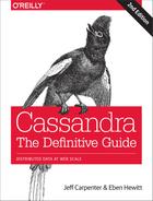
The SimpleStrategy places replicas in a single data center, in a manner that is not aware of their placement on a data center rack. This means that the implementation is theoretically fast, but not if the next node that has the given key is in a different rack than others. This is shown in Figure 7-1.

Figure 7-1. The SimpleStrategy places replicas in a single data center, without respect to topology
What’s happening here is that the next N nodes on the ring are chosen to hold replicas, and the strategy has no notion of data centers. A second data center is shown in the diagram to highlight the fact that the strategy is unaware of it.
NetworkTopologyStrategy
Now let’s say you want to spread replicas across multiple centers in case one of the data centers suffers some kind of catastrophic failure or network outage. The NetworkTopologyStrategy allows you to request that some replicas be placed in DC1, and some in DC2. Within each data center, the NetworkTopologyStrategy distributes replicas on distinct racks, as nodes in the same rack (or similar physical grouping) often fail at the same time due to power, cooling, or network issues.
The NetworkTopologyStrategy distributes the replicas as follows: the first replica is replaced according to the selected partitioner. Subsequent replicas are placed by traversing the nodes in the ring, skipping nodes in the same rack until a node in another rack is found. The process repeats for additional replicas, placing them on separate racks. Once a replica has been placed in each rack, the skipped nodes are used to place replicas until the replication factor has been met.
The NetworkTopologyStrategy allows you to specify a replication factor for each data center. Thus, the total number of replicas that will be stored is equal to the sum of the replication factors for each data center. The results of the NetworkTopologyStrategy are depicted in Figure 7-2.

Figure 7-2. The NetworkTopologyStrategy places replicas in multiple data centers according to the specified replication factor per data center
Additional Replication Strategies
Careful observers will note that there are actually two additional replication strategies that ship with Cassandra: the OldNetworkTopologyStrategy and the LocalStrategy.
The OldNetworkTopologyStrategy is similar to the NetworkTopologyStrategy in that it places replicas in multiple data centers, but its algorithm is less sophisticated. It places the second replica in a different data center from the first, the third replica in a different rack in the first data center, and any remaining replicas by traversing subsequent nodes on the ring.
The LocalStrategy is reserved for Cassandra’s own internal use. As the name implies, the LocalStrategy keeps data only on the local node and does not replicate this data to other nodes. Cassandra uses this strategy for system keyspaces that store metadata about the local node and other nodes in the cluster.
Changing the Replication Factor
You can change the replication factor for an existing keyspace via cqlsh or another client. For the change to fully take effect, you’ll need to run a nodetool command on each of the affected nodes. If you increase the replication factor for a cluster (or data center), run the nodetool repair command on each of the nodes in the cluster (or data center) to make sure Cassandra generates the additional replicas. For as long as the repair takes, it is possible that some clients will receive a notice that data does not exist if they connect to a replica that doesn’t have the data yet.
If you decrease the replication factor for a cluster (or data center), run the nodetool clean command on each of the nodes in the cluster (or data center) so that Cassandra frees up the space associated with unneeded replicas. We’ll learn more about repair, clean, and other nodetool commands in Chapter 11.
As a general guideline, you can anticipate that your write throughput capacity will be the number of nodes divided by your replication factor. So in a 10-node cluster that typically does 10,000 writes per second with a replication factor of 1, if you increase the replication factor to 2, you can expect to do around 5,000 writes per second.
Summary
In this chapter, we looked at how to create Cassandra clusters and add additional nodes to a cluster. We learned how to configure Cassandra nodes via the cassandra.yaml file, including setting the seed nodes, the partitioner, the snitch, and other settings. We also learned how to configure replication for a keyspace and how to select an appropriate replication strategy.