Sizing Your Cluster

An important first step in planning your cluster is to consider the amount of data that it will need to store. You will, of course, be able to add and remove nodes from your cluster in order to adjust its capacity over time, but calculating the initial and planned size over time will help you better anticipate costs and make sound decisions as you plan your cluster configuration.

In order to calculate the required size of the cluster, you’ll first need to determine the storage size of each of the supported tables using the formulas we introduced in Chapter 5. This calculation is based on the columns within each table as well as the estimated number of rows and results in an estimated size of one copy of your data on disk.

In order to estimate the actual physical amount of disk storage required for a given table across your cluster, you’ll also need to consider the replication factor for the table’s keyspace and the compaction strategy in use. The resulting formula for the total size T_t is as follows:

Where S_t is the size of the table calculated using the formula referenced above, RF_k is the replication factor of the keyspace, and CSF_t is a factor representing the compaction strategy of the table, whose value is as follows:

• 2 for the SizeTieredCompactionStrategy. The worst case scenario for this strategy is that there is a second copy of all of the data required for a major compaction.
• 1.25 for other compaction strategies, which have been estimated to require an extra 20% overhead during a major compaction.

Once we know the total physical disk size of the data for all tables, we can sum those values across all keyspaces and tables to arrive at the total for our cluster.

We can then divide this total by the amount of usable storage space per disk to estimate a required number of disks. A reasonable estimate for the usable storage space of a disk is 90% of the disk size.

Note that this calculation is based on the assumption of providing enough overhead on each disk to handle a major compaction of all keyspaces and tables. It’s possible to reduce the required overhead if you can ensure such a major compaction will never be executed by an operations team, but this seems like a risky assumption.

Once you’ve made calculations of the required size and number of nodes, you’ll be in a better position to decide on an initial cluster size. The amount of capacity you build into your cluster is dependent on how quickly you anticipate growth, which must be balanced against cost of additional hardware, whether it be physical or virtual.

Selecting Instances

It is important to choose the right computing resources for your Cassandra nodes, whether you are running on physical hardware or in a virtualized cloud environment. The recommended computing resources for modern Cassandra releases (2.0 and later) tend to differ for development versus production environments:

Development environments

Cassandra nodes in development environments should generally have CPUs with at least two cores and 8 GB of memory. Although Cassandra has been successfully run on smaller processors such as Raspberry Pi with 512 MB of memory, this does require a significant performance-tuning effort.

Production environments

Cassandra nodes in production environments should have CPUs with at least eight cores (although four cores are acceptable for virtual machines), and anywhere from 16 MB to 64 MB of memory.

Storage

There are a few factors to consider when selecting and configuring storage, including the type and quantities of drives to use:

HDDs versus SSDs

Cassandra supports both hard disk drives (HDDs, also called “spinning drives”) and solid state drives (SSDs) for storage. Although Cassandra’s usage of append-based writes is conducive to sequential writes on spinning drives, SSDs provide higher performance overall because of their support for low-latency random reads.

Historically, HDDs have been the more cost-effective storage option, but the cost of using SSDs has continued to come down, especially as more and more cloud platform providers support this as a storage option.

Disk configuration

If you’re using spinning disks, it’s best to use separate disks for data and commit log files. If you’re using SSDs, the data and commit log files can be stored on the same disk.

JBOD versus RAID

Traditionally, the Cassandra community has recommended using multiple disks for data files, with the disks configured as a Redundant Array of Independent Disks (RAID). Because Cassandra uses replication to achieve redundancy across multiple nodes, the RAID 0 (or “striped volume”) configuration is considered sufficient.

More recently, Cassandra users have been using a Just a Bunch of Disks (JBOD) deployment style. The JBOD approach provides better performance and is a good choice if you have the ability to replace individual disks.

Avoid shared storage

When selecting storage, avoid using Storage Area Networks (SAN) and Network Attached Storage (NAS). Neither of these storage technologies scale well—they consume additional network bandwidth in order to access the physical storage over the network, and they require additional I/O wait time on both reads and writes.

Network

Because Cassandra relies on a distributed architecture involving multiple networked nodes, here are a few things you’ll need to consider:

Throughput

First, make sure your network is sufficiently robust to handle the traffic associated with distributing data across multiple nodes. The recommended network bandwidth is 1 GB or higher.

Network configuration

Make sure that you’ve correctly configured firewall  rules and IP addresses for your nodes and network appliances to allow traffic on the ports used for the CQL native transport, inter-node communication (the listen_address), JMX, and so on. This includes networking between data centers (we’ll discuss cluster topology momentarily).

The clocks on all nodes should be synchronized using Network Time Protocol (NTP) or other methods. Remember that Cassandra only overwrites columns if the timestamp for the new value is more recent than the timestamp of the existing value. Without synchronized clocks, writes from nodes that lag behind can be lost.

Avoid load balancers

Load balancers are a feature of many computing environments. While these are frequently useful to spread incoming traffic across multiple service or application instances, it’s not recommended to use load balancers with Cassandra. Cassandra already provides its own mechanisms to balance network traffic between nodes, and the DataStax drivers spread client queries across replicas, so strictly speaking a load balancer won’t offer any additional help. Besides this, putting a load balancer in front of your Cassandra nodes actually introduces a potential single point of failure, which could reduce the availability of your cluster.

Timeouts

If you’re building a cluster that spans multiple data centers, it’s a good idea to measure the latency between data centers and tune timeout values in the cassandra.yaml file accordingly.

A proper network configuration is key to a successful Cassandra deployment, whether it is in a private data center, a public cloud spanning multiple data centers, or even a hybrid cloud environment.

Amazon Web Services

Amazon Web Services (AWS) has been a popular deployment option for Cassandra, as evidenced by the presence of AWS-specific extensions in the Cassandra project such as the Ec2Snitch, Ec2MultiRegionSnitch, and the EC2MultiRegion​Address​Translator in the DataStax Java Driver.

Cluster layout

AWS is organized around the concepts of regions and availability zones, which are typically mapped to the Cassandra constructs of data centers and racks, respectively. A sample AWS cluster topology spanning the us-east-1 (Virginia) and eu-west-1 (Ireland) regions is shown in Figure 14-1. The node names are notional—this naming is not a required convention.

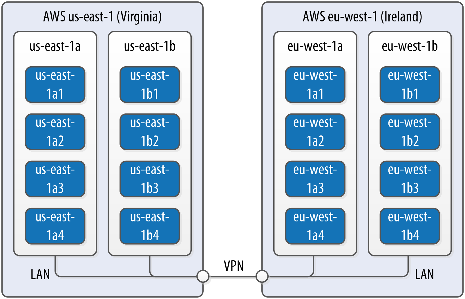
Figure 14-1. Topology of a cluster in two AWS regions

EC2 instances

The Amazon Elastic Compute Cloud (EC2) provides a variety of different virtual hardware instances grouped according to various classes. The two classes most frequently recommended for Cassandra deployments are the M-class and the I-class.

M-class instances are general-purpose instances that balance compute, memory, and network resources and are generally acceptable for development and light production environments. Later M-class instances such as M3 and M4 are SSD-backed.

The I-class instances are all SSD-backed and designed for high I/O. These instances come at a higher cost that generally pays off for heavily loaded production clusters.

You can find more information about the various instance types available at https://aws.amazon.com/ec2/instance-types.

DataStax Enterprise provides a prebuilt Amazon Machine Image (AMI) to simplify deployment (an AMI for DataStax Community Edition was discontinued after the Cassandra 2.1 release).

Data storage

Historically, the recommended disk option in AWS was to use ephemeral storage attached to each instance. The drawback of this is that if an instance on which a node is running is terminated (as happens occasionally in AWS), the data is lost. By late 2015, the network-attached storage known as Elastic Block Store (EBS) has been proven to provide a reliable place to store data that doesn’t go away when EC2 instances are dropped, at the cost of additional latency. 

AWS Services such as S3 and Glacier are a good option for short- to medium-term and long-term storage of backups, respectively.

Networking

If you’re running a multi-region configuration, you’ll want to make sure you have adequate networking between the regions. Many have found that using elements of the AWS Virtual Private Cloud (VPC) provides an effective way of achieving reliable, high-throughput connections between regions. AWS Direct Connect provides dedicated private networks, and there are virtual private network (VPN) options available as well. These services of course come at an additional cost.

If you have a single region deployment or a multi-region deployment using VPN connections between regions, use the Ec2Snitch. If you have a multi-region deployment that uses public IP between regions, use the Ec2MultiRegionSnitch. For either snitch, increasing the phi_convict_threshold value in the cassandra.yaml file to 12 is generally recommended in the AWS network environment.

Microsoft Azure

DataStax and Microsoft have partnered together to help improve deployment of Cassandra in Microsoft’s Azure on both Windows and Ubuntu Linux OSs.

Cluster layout

Azure provides data centers in locations worldwide, using the same term “region” as AWS. The concept of availability sets is used to manage collections of VMs. Azure manages the assignment of the VMs in an availability set across update domains, which equate to Cassandra’s racks.

Virtual machine instances

Similar to AWS, Azure provides several classes of VMs. The D series, D series v2, and G series machines are all SSD-backed instances appropriate for Cassandra deployments. The G series VMs provide additional memory as required for integrations such as those described next. You can find more information about Azure VM types at https://azure.microsoft.com/en-us/pricing/details/virtual-machines.

Data storage

Azure provides a standard SSD capability on the previously mentioned instances. In addition, you can upgrade to use Premium Storage, which provides network-attached SSDs in larger sizes up to 1 TB.

Networking

Public IP addresses are recommended for both single-region and multi-region deployments. Use the GossipingPropertyFileSnitch to allow your nodes to detect the cluster topology. Networking options between regions include VPN Gateways and the Express Route, which provides up to 2 GB/s throughput.

Google Cloud Platform

Google Cloud Platform provides cloud computing, application hosting, networking, storage, and various Software-as-a-Service (SaaS) offerings such as Google’s Translate and Prediction APIs. 

Cluster layout

The Google Compute Environment (GCE) provides regions and zones, corresponding to Cassandra’s data centers and racks, respectively.

Virtual machine instances

GCE’s n1-standard and n1-highmemory machine types are recommended for Cassandra deployments. You can launch Cassandra quickly on the Google Cloud Platform using the Cloud Launcher. For example if you search the launcher at https://cloud.google.com/launcher/?q=cassandra, you’ll find options for creating a cluster in just a few button clicks.

Data storage

GCE provides both spinning disk (pd-hdd) and solid state disk options for both ephemeral drives (local-ssd) and network-attached drives (pd-ssd). There are three storage options that can be used to store Cassandra backups, each with different cost and availability profiles: Standard, Durable Reduced Availability (DRA), and Nearline.

Networking

The GoogleCloudSnitch is a custom snitch designed just for the GCE. VPN networking is available between regions.

Apache Lucene, SOLR, and Elasticsearch

One of the features that is commonly required in applications built on top of Cassandra is full text searching. This capability can be added to Cassandra via Apache Lucene, which provides an engine for distributed indexing and searching, and its subproject, Apache Solr, which adds REST and JSON APIs to the Lucene search engine.

Elasticsearch is another popular open source search framework built on top of Apache Lucene. It supports multitenancy and provides Java and JSON over HTTP APIs.

Stratio has provided a plugin that can be used to replace Cassandra’s standard secondary index implementation with a Lucene index. When using this integration, there is a Lucene index available on each Cassandra node that provides high performance search capability.

Apache Hadoop

Apache Hadoop is a framework that provides distributed storage and processing of large data sets on commodity hardware. This work originated at Google in the early 2000s. Google found that several internal groups had been implementing similar functionality for data processing, and that these tools commonly had two phases: a map phase and a reduce phase. A map function operates over raw data and produces intermediate values. A reduce function distills those intermediate values, producing the final output. In 2006, Doug Cutting wrote open source implementations of the Google File System, and MapReduce, and thus, Hadoop was born.

Similar to Cassandra, Hadoop uses a distributed architecture with nodes organized in clusters. The typical integration is to install Hadoop on each Cassandra node that will be used to provide data. You can use Cassandra as a data source by running a Hadoop Task Tracker and Data Node on each Cassandra node. Then, when a MapReduce job is initiated (typically on a node external to the Cassandra cluster), the Job Tracker can query Cassandra for data as it tracks map and reduce tasks, as shown in Figure 14-2.

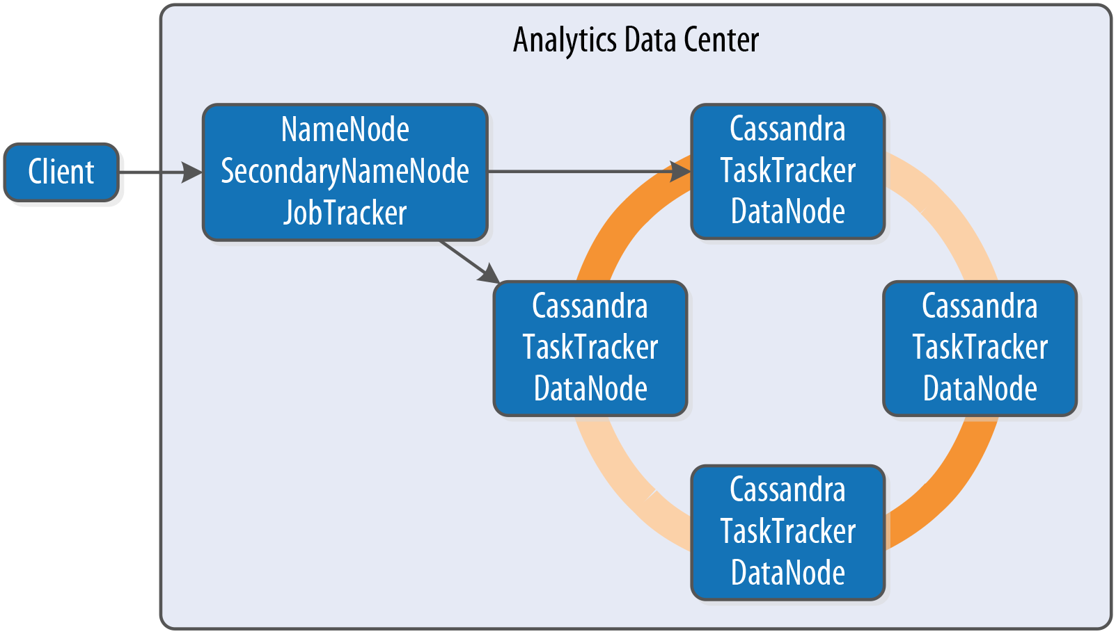
Figure 14-2. Topology of a Hadoop-Cassandra cluster

Starting in the late 2000s, Hadoop has been a huge driver of interest and growth in the Big Data community. Due to its popularity, a large ecosystem of extensions has developed around Hadoop, such as Apache Pig, which provides a framework and language for data analysis, and Apache Hive, a data warehouse tool. The Hadoop community has begun moving away from MapReduce because of its relatively slow performance (all data is written to disk, even for intermediate processing steps), high memory use, non-intuitive API, and batch-only processing mode. For this reason, the emergence of the Apache Spark project has been a significant development.

Apache Spark

with Patrick McFadin

Apache Spark is an emerging data analytics framework that provides a massively parallel processing framework to enable simple API calls across large volumes of data. Originally developed in 2009 at UC Berkeley as an improvement to MapReduce, Spark was open sourced in 2010, and became an Apache project in 2014.

Unlike Hadoop, which writes intermediate results to disk, the Spark core processing engine is designed to maximize memory usage while minimizing disk and network access. Spark uses streaming instead of batch-oriented processing to achieve processing speeds up to 100 times faster than Hadoop. In addition, Spark’s API is much simpler to use than Hadoop.

The basic unit of data representation in Spark is the Resilient Distributed Dataset (RDD). The RDD is a description of the data to be processed, such as a file or data collection. Once an RDD is created, the data contained can be transformed with API calls as if all of the data were contained in a single machine. However, in reality, the RDD can span many nodes in the network by partitioning. Each partition can be operated on in parallel to produce a final result. The RDD supports the familiar map and reduce operations plus additional operations such as count, filter, union, and distinct. For a full list of transformations, see the Spark documentation.

In addition to the core engine, Spark includes further libraries for different types of processing requirements. These are included as subprojects that are managed separately from Spark core, but follow a similar release schedule:

• SparkSQL provides familiar SQL syntax and relational queries over structured data.
• MLlib is Spark’s machine learning library.
• SparkR provides support for using the R statistics language in Spark jobs.
• GraphX is Spark’s library for graph and collection analytics.
• Spark Streaming provides near real-time processing of live data streams.

Deploying Spark with Cassandra

Cassandra places data per node based on token assignment. This existing data distribution can be used as an advantage to parallelize Spark jobs. Because each node contains a subset of the cluster’s data, the recommended configuration for Spark-Cassandra integrations is to co-locate a Spark Worker on each Cassandra node in a data center, as shown in Figure 14-3.

Figure 14-3. Topology of a Spark-Cassandra cluster

When a job is submitted to the Spark Master, the Spark Workers on each node spawn Spark Executors to complete the work. Using the spark-cassandra-connector as a conduit,  he data required for each job is sourced from the local node as much as possible. We’ll learn more about the connector momentarily.

Because each node contains a portion of the entire data in the cluster, each Spark Worker will only need to process that local subset of data. An example is a count action on a table. Each node will have a range of the table’s data. The count is calculated locally and then merged from every node to produce the total count.

This design maximizes data locality, resulting in improved throughput and lower resource utilization for analytic jobs. The Spark Executors only communicate over the network when data needs to be merged from other nodes. As cluster sizes get larger, the efficiency gains of this design are much more pronounced.

<dependency>
    <groupId>org.apache.spark</groupId>
    <artifactId>spark-core_2.10</artifactId>
    <version>1.5.2</version>
</dependency>
<dependency>
    <groupId>com.datastax.spark</groupId>
    <artifactId>spark-cassandra-connector_2.10</artifactId>
    <version>1.5.0</version>
</dependency>

val conf = new SparkConf(true)
   .set("spark.cassandra.connection.host", "127.0.0.1")
   .setMaster("local[*]")
   .setAppName(getClass.getName)
   // Optionally     
   .set("cassandra.username", "cassandra")     
   .set("cassandra.password", "cassandra")

val sc = new SparkContext(conf)

val rdd = sc.cassandraTable("reservation", 
  "reservations_by_hotel_date")

println("Number of reservations: " + rdd.count)

val rdd = sc.cassandraTable("reservation", 
  "reservations_by_hotel_date")
  .select("hotel_id", "confirm_number")
  .where("end_date = ?", "2016-09-08")

// Invoke the action to run the spark job
rdd.toArray.foreach(println)

// Create a collection of guests with simple identifiers
val collection = sc.parallelize(Seq(("1", "Delaney", "McFadin"), 
  ("2", "Quinn", "McFadin")))

// Save to the guests table
collection.saveToCassandra("reservation", "guests", 
  SomeColumns("guest_id", "first_name", "last_name"))

// Use the SparkContext to create a CassandraSQLContext
val cc = new CassandraSQLContext(sc)

// Set the keyspace
cc.setKeyspace("reservation")
val rdd = cc.cassandraSql("
SELECT hotel_id, confirm_number
FROM reservations_by_hotel_date
WHERE end_date = '2016-09-08'  
ORDER BY hotel_id")

// Perform action to run SQL job
rdd.collect().foreach(println)