
Chapter 3. Sharing, Scaling and Elasticity Patterns

Load Balanced Virtual Server Instances
Load Balanced Virtual Switches
Cross-Storage Device Vertical Tiering
Intra-Storage Device Vertical Data Tiering
This collection of design patterns focuses on providing solutions for maximizing the potential usage of available IT resources in response to unpredictable usage requirements across multiple cloud consumers. Shared Resources (17), Dynamic Data Normalization (71), Memory Over-Committing (86), and NIC Teaming (90) directly enable and support the realization of multitenancy over large pooled resources, whereas ubiquitous cloud consumer access is enabled through the application of the Broad Access (93) pattern.
The majority of patterns in this chapter directly or indirectly enable the elasticity characteristic of cloud computing to support the automated ability of a cloud to transparently scale IT resources, as required in response to runtime conditions or as pre-determined by the cloud consumer or cloud provider.

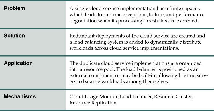
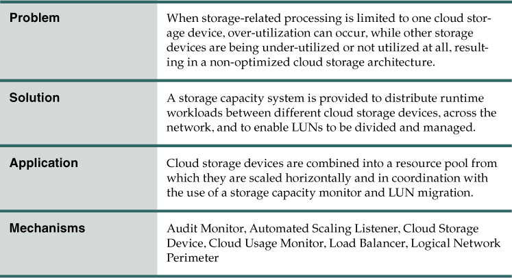
Problem
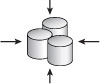
Organizations commonly purchase physical on-premise IT resources, such as physical servers and storage devices, and allocate each to specific applications, users, or other types of consumers (Figure 3.1). The narrow scope of some IT resource usage results in the IT resource’s overall capacity rarely being fully used. Over time, the processing potential of each IT resource is not reached. Consequently, the return on the investment of each IT resource is also not fully realized. The longer these types of dedicated IT resources are used, the more wasteful they become, and more opportunities to further leverage their potential are lost.

Figure 3.1 Each cloud consumer is allocated a dedicated physical server. It is likely that, over time, a significant amount of the physical servers’ combined capacity will be under-utilized.
Solution
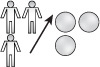
Virtual instances of physical IT resources are created and shared by multiple consumers, potentially to the extent to which the capacity of the physical IT resource can support (Figure 3.2). This maximizes the utilization of each physical IT resource, thereby also maximizing the return on its investment.

Figure 3.2 Each cloud consumer is allocated a virtual server instance of a single underlying physical server. In this case, the physical server is likely greater than if each cloud consumer were given its own physical server. However, the cost of one high-capacity physical server is lower than four medium-capacity physical servers and its processing potential will be utilized to a greater extent.
This pattern further forms the fundamental basis of a model by which virtual instances of the physical IT resource can be used (and leased) temporarily.
Application
The most common technology used to apply this pattern is virtualization. The specific components and mechanisms that are used depend on what type of IT resource needs to be shared. For example, the virtual server mechanism is used to share a physical server’s processing capacity and the hypervisor mechanism is utilized to create instances of the virtual server. The VIM component can be further incorporated to manage hypervisors, virtual server instances, and their distribution.
It is important to note how the Shared Resources pattern is positioned among compound patterns, especially given its fundamental nature in relation to cloud platforms:
The Shared Resources pattern is:
• an optional member of the Private Cloud (474) compound pattern because, although common in private clouds, the virtualization of physical IT resources for cloud consumer sharing purposes is an option that can be chosen in support of the business requirements of the organization acting as cloud provider.
• a required member of the Public Cloud (476) compound pattern because of its inherent need to share IT resources to numerous cloud consumers.
• an optional member of the IaaS (482) compound pattern because the cloud provider may allow the cloud consumer access to administer raw physical IT resources and the decision of whether and how to use virtualization technology is left to the cloud consumer.
• a required member of the PaaS (480) compound pattern because the ready-made environment mechanism itself is naturally virtualized.
• a required member of the SaaS (478) compound pattern because SaaS offerings are naturally virtualized.
• a required member of the Multitenant Environment (486) compound pattern because this pattern provides a cloud technology architecture that specifically addresses the sharing of IT resources.
The sharing of IT resources introduces risks and challenges:
• One physical IT resource can become a single point of failure for multiple virtual IT resources and multiple corresponding cloud consumers.
• The virtualized physical IT resource may become over-utilized and therefore unable to fulfill all of the processing demands of its virtualized instances. This is referred to as a resource constraint and represents a condition that can lead to degradation of performance and various runtime exceptions.
• The virtualized instances of an underlying physical IT resource shared by multiple cloud consumers can introduce overlapping trust boundaries that can pose a security concern.
These and other problems raised by the application of this pattern are addressed by other patterns, such as Resource Pooling (99) and Resource Reservation (106).
Mechanisms
• Audit Monitor – When the Shared Resources pattern is applied, it can change how and where data is processed and stored. This may require the use of an audit monitor mechanism to ensure that the utilization of shared IT resources does not inadvertently violate legal requirements or regulations.
• Cloud Storage Device – This mechanism represents a common type of IT resource that is shared by the application of this pattern.
• Cloud Usage Monitor – Various cloud usage monitors may be involved with tracking the shared usage of IT resources.
• Hypervisor – A hypervisor can provide virtual servers with access to shared IT resources hosted by the hypervisor.
• Logical Network Perimeter – This mechanism provides network-level isolation that helps protect shared IT resources and their cloud consumers.
• Resource Replication – The resource replication mechanism may be used to generate new instances of IT resources made available for shared usage.
• Virtual CPU – This mechanism is used to share the hypervisor’s physical CPU between virtual servers.
• Virtual Infrastructure Manager (VIM) – This mechanism is used to configure how physical resources are to be shared between virtual servers in order to send the configurations to the hypervisors.
• Virtual RAM – This mechanism is used to determine how a hypervisor’s physical memory is to be shared between virtual servers.
• Virtual Server – Virtual servers may be shared or may host shared IT resources.


Problem
IT resources that are shared or are made available to consumers with unpredictable usage requirements can become over-utilized when usage demands near or exceed their capacities (Figure 3.3). This can result in runtime exceptions and failure conditions that cause the affected IT resources to reject consumer requests or shut down altogether.

Figure 3.3 A group of cloud service consumers simultaneously access Cloud Service A, which is hosted by Virtual Server A. Another virtual server is available but is not being utilized. As a result, Virtual Server A is over-utilized.
Solution
The IT resource is horizontally scaled via the addition of one or more identical IT resources and a load balancing system further extends the cloud architecture to provide runtime logic capable of evenly distributing the workload across all available IT resources (Figure 3.4). This minimizes the chances that any one of the IT resources will be over-utilized (or under-utilized).

Figure 3.4 A redundant copy of Cloud Service A is implemented on Virtual Server B. The load balancer intercepts the cloud service consumer requests and directs them to both Virtual Server A and B to ensure even distribution of the workload.
Application
This pattern is primarily applied via the use of the load balancer mechanism, of which variations with different types of load balancing algorithms exist. The automated scaling listener mechanism can also be used in a similar capacity to respond when an IT resource’s thresholds are reached.
In addition to the distribution of conventional cloud service access and data exchanges, this pattern can also be applied to the load balancing of cloud storage devices and connectivity devices.
Mechanisms
• Audit Monitor – When distributing runtime workloads, the types of IT resources processing data and the geographical location of the IT resources (and the data) may need to be monitored for legal and regulatory requirements.
• Cloud Storage Device – This is one type of mechanism that may be used to distribute workload as a result of the application of this pattern.
• Cloud Usage Monitor – Various monitors may be involved with the runtime tracking of workload and data processing as part of a cloud architecture resulting from the application of this pattern.
• Hypervisor – Workloads between hypervisors and virtual servers hosted by hypervisors may need to be distributed.
• Load Balancer – This is a fundamental mechanism used to establish the base workload balancing logic in order to carry out the distribution of the workload.
• Logical Network Perimeter – The logical network perimeter isolates cloud consumer network boundaries in relation to how and to where workloads may be distributed.
• Resource Cluster – Clustered IT resources in active/active mode are commonly used to support the workload balancing between the different cluster nodes.
• Resource Replication – This mechanism may generate new instances of virtualized IT resources in response to runtime workload distribution demands.
• Virtual Server – Virtual servers may be the target of workload distribution or may themselves be hosting IT resources that are part of workload distribution architectures.

Problem
Manually preparing or extending IT resources in response to workload fluctuations is time-intensive and unacceptably inefficient. Determining when to add new IT resources to satisfy anticipated workload peaks is often speculative and generally risky. These additional IT resources can either remain under-utilized (and a failed financial investment), or fail to alleviate runtime performance and reliability problems when demand exceeds even the addition of their capacity.
The following steps are shown in Figures 3.5 and 3.6:
1. The cloud provider offers cloud services to cloud consumers.
2. Cloud consumers can scale the cloud services, as needed.
3. Over time, the number of cloud consumers increases.
4. The cloud provider’s virtual server is overwhelmed with the increased workload capacity.
5. The cloud provider brings a new, higher-capacity server online to handle an increased workload.
6. Because the required IT resources are not organized for sharing and are unprepared for allocation, the virtual server must have the operating system, required applications, and cloud services installed after being created.
7. Once the new server is ready, the old server is taken offline.
8. Now service requests are redirected to the new server.
9. After the peak usage period has ended, the number of cloud consumers and service requests naturally decrease.
10. Without properly implementing a process of under-utilized IT resource recovery, the new server’s sizable workload capacity will not be fully utilized.

Figure 3.5 A non-dynamic cloud architecture in which vertical scaling is carried out in response to usage fluctuations (Part I).

Figure 3.6 A non-dynamic cloud architecture in which vertical scaling is carried out in response to usage fluctuations (Part II).
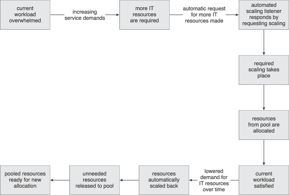
Solution
A system of predefined scaling conditions that trigger the dynamic allocation of IT resources can be introduced (Figure 3.7). The IT resources are allocated from resource pools to allow for variable utilization as dictated by demand fluctuations. Unneeded IT resources are efficiently reclaimed without requiring manual interaction.
Application
The fundamental Dynamic Scalability pattern primarily relies on the application of Resource Pooling (99) and the implementation of the automated scaling listener.
The automated scaling listener is configured with workload thresholds that determine when new IT resources need to be included in the workload processing. The automated scaling listener can further be provided with logic that allows it to verify the extent of additional IT resources a given cloud consumer is entitled to, based on its leasing arrangement with the cloud provider.
The following types of dynamic scaling are common:
• Dynamic Horizontal Scaling – In this type of dynamic scaling the number of IT resource instances is scaled to handle fluctuating workloads. The automatic scaling listener monitors requests and, if scaling is required, signals a resource replication mechanism to initiate the duplication of the IT resources, as per requirements and permissions. (Figures 3.8 to 3.10 demonstrate this type of scaling.)
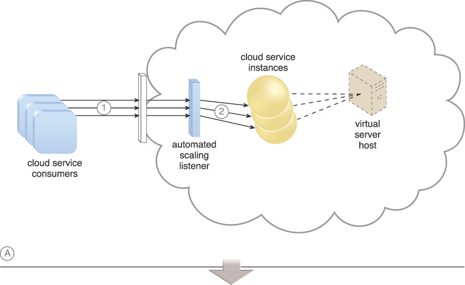
Figure 3.8 An example of a dynamic scaling architecture involving an automated scaling mechanism (Part I).

Figure 3.9 An example of a dynamic scaling architecture involving an automated scaling mechanism (Part II).
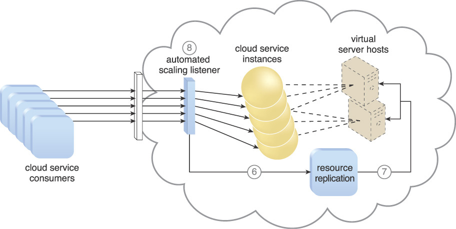
Figure 3.10 An example of a dynamic scaling architecture involving an automated scaling mechanism (Part III).
• Dynamic Vertical Scaling – This type of scaling occurs when there is a need to increase the processing capacity of a single IT resource. For instance, if a virtual server is being overloaded, it can dynamically have its memory increased or it may have a processing core added.
• Dynamic Relocation – The IT resource is relocated to a higher capacity host. For example, there may be a need to move a cloud service database from a tape-based SAN storage device with 4 Gbps I/O capacity to another disk-based SAN storage device with 8 Gbps I/O capacity.
Figures 3.8 to 3.10 demonstrate dynamic horizontal scaling in the following steps:
1. Cloud service consumers are sending requests to a cloud service.
2. The automated scaling listener monitors the cloud service to determine if pre-defined capacity thresholds are being exceeded.
3. The number of service requests coming from cloud service consumers further increases.
4. The workload exceeds the performance thresholds of the automated scaling listener. It determines the next course of action based on a pre-defined scaling policy.
5. If the cloud service implementation is deemed eligible for additional scaling, the automated scaling listener initiates the scaling process.
6. The automated scaling listener sends a signal to the resource replication mechanism.
7. The resource replication mechanism then creates more instances of the cloud service.
8. Now that the increased workload is accommodated, the automated scaling listener resumes monitoring and the detracting or adding of necessary IT resources.
Mechanisms
• Automated Scaling Listener – The automated scaling listener is directly associated with the Dynamic Scalability pattern in that it monitors and compares workloads with predefined thresholds to initiate scaling in response to usage fluctuations.
• Cloud Storage Device – This mechanism and the data it stores may be scaled by the system established by this pattern.
• Cloud Usage Monitor – As per the automated scaling listener, cloud usage monitors are used to track runtime usage to initiate scaling in response to fluctuations.
• Hypervisor – The hypervisor may be invoked by a dynamic scalability system to create or remove virtual server instances. Alternatively, the hypervisor itself may be scaled.
• Pay-Per-Use Monitor – The pay-per-use monitor collects usage cost information in tandem with how IT resources are scaled.
• Resource Replication – This mechanism supports dynamic horizontal scaling by replicating IT resources, as required.
• Virtual Server – The virtual server may be scaled by the system established by this pattern.

Problem
Regardless of the processing capacity of its immediate hosting environment, a cloud service architecture may inherently be limited in its ability to accommodate high volumes of concurrent cloud service consumer requests. The cloud service’s processing restrictions may be such that it is unable to leverage underlying cloud-based IT resources that normally support dynamic scalability. For example, the processing restrictions may originate from its architectural design, the complexity of its application logic, or inhibitive programming algorithms it is required to carry out at runtime. Such a cloud service may be forced to reject cloud service consumer requests when its processing capacity thresholds are reached (Figure 3.11).

Figure 3.11 A single cloud service implementation reaches its runtime processing capacity and consequently rejects subsequent cloud service consumer requests.
Solution
Redundant implementations of the cloud service are created, each located on a different hosting server. A load balancer is utilized to intercept cloud service consumer requests in order to evenly distribute them across the multiple cloud service implementations (Figure 3.12).
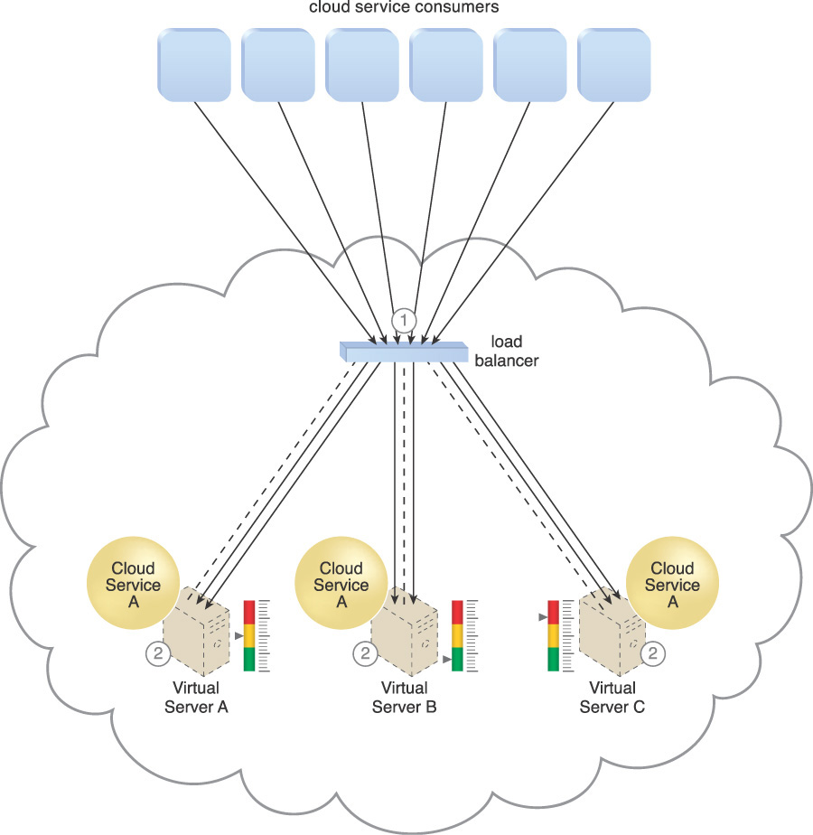
Figure 3.12 The load balancing agent intercepts messages sent by cloud service consumers (1) and forwards the messages at runtime to the virtual servers so that the workload processing is horizontally scaled (2).
Application
Depending on the anticipated workload and the processing capacity of hosting server environments, multiple instances of each cloud service implementation may be generated in order to establish pools of cloud services that can more efficiently respond to high volumes of concurrent requests.
The load balancer may be positioned independently from the cloud services and their hosting servers, as shown in Figure 3.12, or it may be built-in as part of the application or server’s environment. In the latter case, a primary server with the load balancing logic can communicate with neighboring servers to balance the workload, as shown in Figure 3.13.
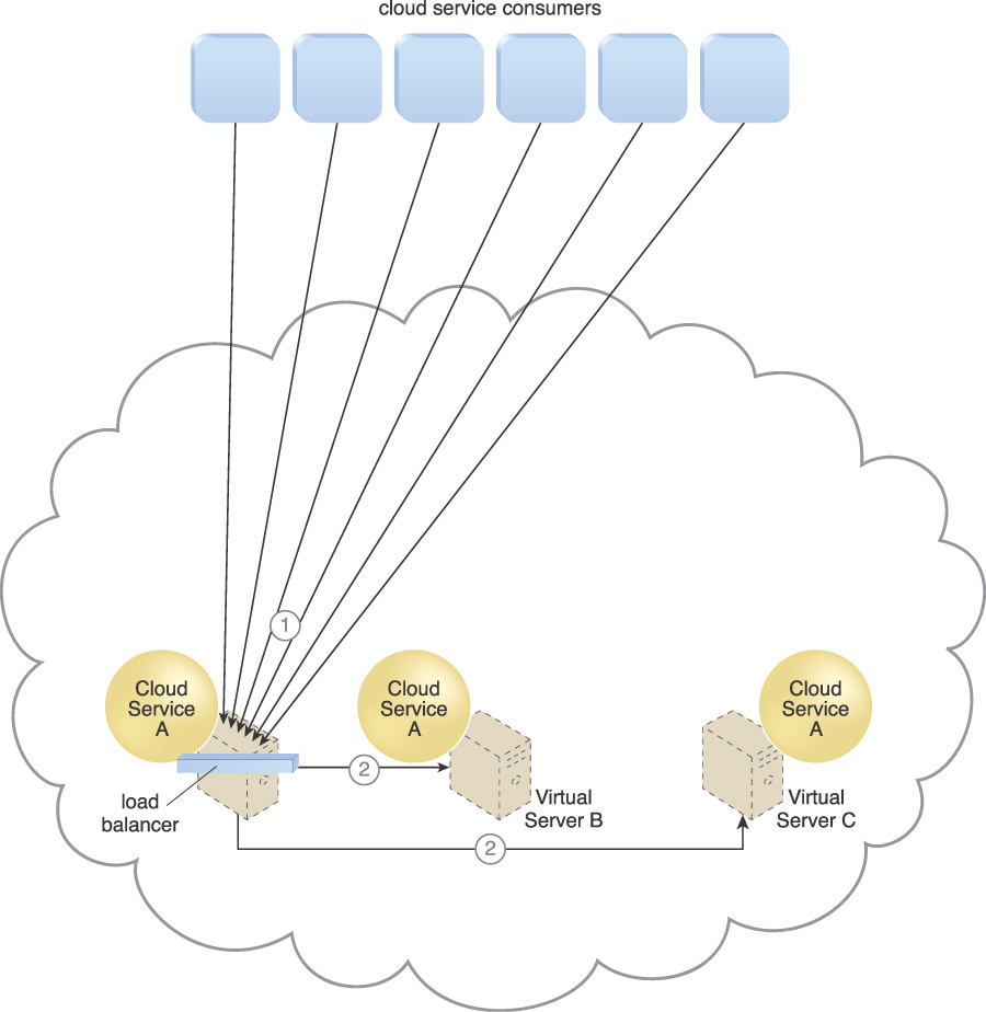
Figure 3.13 Cloud consumer requests are sent to Cloud Service A on Virtual Server A (1). The cloud service implementation includes built-in load balancing logic that is capable of distributing requests to the neighboring Cloud Service A implementations on Virtual Servers B and C (2).
For this pattern to be applied, a server group needs to be created and configured, so that server group members can be associated with the load balancer. The paths of cloud service consumer requests to be sent through the load balancer need to be set and the load balancer needs to be configured to evaluate each cloud service implementation’s capacity on a regular basis.
Mechanisms
• Cloud Usage Monitor – In addition to performing various runtime monitoring and usage data collection tasks, cloud usage monitors may be involved with monitoring cloud service instances and their respective IT resource consumption levels.
• Load Balancer – This represents the fundamental mechanism used to apply this pattern in order to establish the necessary horizontal scaling functionality.
• Resource Cluster – Active-active cluster groups may be incorporated in a service load balancing architecture to help balance workloads across different members of the cluster.
• Resource Replication – Resource replication is utilized to keep cloud service implementations synchronized.
Elastic Resource Capacity

How can the processing capacity of virtual servers be dynamically scaled in response to fluctuating IT resource usage requirements?

Problem
When the processing capacity of a virtual server is reached at runtime, it becomes unavailable, resulting in scalability limitations and inhibiting the performance and reliability of its hosted IT resources (Figure 3.14).

Figure 3.14 After the virtual server hosting the cloud service reaches its processing limit, subsequent cloud service consumer requests cannot be fulfilled.
Solution
Pools of CPUs and RAM are established for shared allocation. The runtime processing of a virtual server is monitored so that prior to capacity thresholds being met, additional processing power from the resource pool can be leveraged via dynamic allocation to the virtual server. This vertically scales the virtual server and, consequently, its hosted applications and IT resources as well.
Application
Resource Pooling (99) is applied to provision the necessary IT resource pools, and Dynamic Scalability (25) is applied to establish the automated scaling listener mechanism as an intermediary between cloud service consumers and any IT resources hosted by the virtual server that need to be accessed. Automated Administration (310) is further applied because intelligent automation engine scripts are needed to signal scaling requirements to the resource pool.
The following steps are shown in Figures 3.15 and 3.16:
1. Resource pools providing CPUs and RAM memory have been implemented and configured.
2. Cloud service consumers are actively sending requests.
3. The automated scaling listener is monitoring the requests.
4. An intelligent automation engine script is deployed with workflow logic capable of notifying the resource pool using allocation requests.
5. Cloud service consumer requests increase.
6. The automated scaling listener signals the intelligent automation engine to execute the script.
7. The script runs the workflow logic that signals the hypervisor to allocate more IT resources from the resource pools.
8. The hypervisor allocates additional CPU and RAM to the virtual server, enabling it to handle the increased workload.

Figure 3.15 The application of the Elastic Resource Capacity pattern on a sample cloud architecture (Part I).
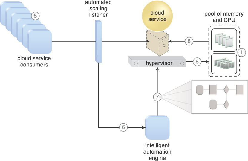
Figure 3.16 The application of the Elastic Resource Capacity pattern on a sample cloud architecture (Part II).
This type of cloud architecture may also be designed so that the intelligent automation engine script sends its scaling request via the VIM instead of directly to the hypervisor. Furthermore, in order to support dynamic resource allocation, virtual servers participating in elastic resource allocation systems may need to be rebooted for the allocation to take effect.
Mechanisms
• Automated Scaling Listener – The Elastic Resource Capacity pattern is reliant on the automated scaling listener mechanism for monitoring the workload and initiating the scaling process by indicating the type of scaling that is required.
• Cloud Usage Monitor – This mechanism is associated with the Elastic Resource Capacity pattern in how the cloud usage monitor collects the resource usage information of the allocated and released IT resources before, during, and after scaling, to help determine the future processing capacity thresholds of the virtual servers.
• Hypervisor – The hypervisor is responsible for hosting the virtual servers that house the resource pools that undergo dynamic reallocation. This mechanism allocates computing capacity to virtual servers according to demand, in alignment with the configurations and policies defined via the virtual infrastructure manager (VIM) by the cloud provider or resource administrator.
• Live VM Migration – If a virtual server requires additional capacity that cannot be accommodated by the current hypervisor, this mechanism is used to migrate the virtual server to another hypervisor that can offer the required capacity before adding more computing capacity at the destination.
• Pay-Per-Use Monitor – The pay-per-use monitor is related to this pattern in how the monitor is responsible for collecting all of the resource usage cost information, in parallel with the cloud usage monitor.
• Resource Replication – Resource replication is associated with this pattern in how this mechanism is used to instantiate new instances of the service or application, virtual server, or both.
• Virtual CPU – Processing power is added to virtual servers in units of gigahertz or megahertz, via the use of virtual CPU. This mechanism is used for allocating CPU according to the schedule and processing cycle of the virtual servers.
• Virtual Infrastructure Manager (VIM) – Virtual CPU and memory configurations are performed via this mechanism and forwarded to the hypervisors.
• Virtual RAM – Virtual servers are allocated the required memory via the use of this mechanism, which allows resource administrators to virtualize the physical memory installed on physical servers and share the virtualized memory between virtual servers. This mechanism also allows resource administrators to allocate memory in quantities greater than the amount of physical memory installed on the physical servers.
• Virtual Server – The Elastic Resource Capacity pattern relates to this mechanism in how virtual servers host the services and applications that are consumed by cloud consumers, and experience workload distribution when processing capacities have been reached.
Elastic Network Capacity
How can network bandwidth be allocated to align with actual usage requirements?

Problem
Even if IT resources are scaled on-demand by a cloud platform, performance and scalability can still be inhibited when remote access to the IT resources is impacted by network bandwidth limitations (Figure 3.17).

Figure 3.17 A scenario whereby a lack of available bandwidth causes performance issues for cloud consumer requests.
Solution
A system is established in which additional bandwidth is allocated dynamically to the network to avoid runtime bottlenecks. This system ensures that individual cloud consumer traffic flows are isolated and that each cloud consumer is using a different set of network ports.
Application
The automated scaling listener mechanism and intelligent automation engine scripts are used to detect when traffic reaches a bandwidth threshold and to then respond with the dynamic allocation of additional bandwidth and/or network ports.
The cloud architecture may be equipped with a network resource pool containing network ports that are made available for shared usage. The automated scaling listener monitors workload and network traffic and signals the intelligent automation engine to increase or decrease the number of allocated network ports and/or bandwidth in response to usage fluctuations.
Note that when applying this pattern at the virtual switch level, the intelligent automation engine may need to run a separate script that adds physical uplinks specifically to the virtual switch. Alternatively, Direct I/O Access (169) can also be applied to increase network bandwidth that is allocated to the virtual server.
Mechanisms
• Automated Scaling Listener – The automated scaling listener is responsible for monitoring the workload and initiating the scaling of the network capacity.
• Cloud Usage Monitor – Cloud usage monitors may be involved with monitoring elastic network capacity before, during, and after scaling.
• Hypervisor – The hypervisor is used by this pattern to provide virtual servers with access to the physical network via virtual switches and physical uplinks.
• Logical Network Perimeter – The logical network perimeter establishes the boundaries necessary to allow for allocated network capacity to be made available to specific cloud consumers.
• Pay-Per-Use Monitor – This monitor keeps track of billing-related data pertaining to the dynamic network bandwidth consumption that occurs as a result of the application of this pattern.
• Resource Replication – Resource replication is utilized to add network ports to physical and virtual servers in response to workload demands.
• Virtual Server – Virtual servers host the IT resources and cloud services to which network resources are allocated and are themselves affected by the scaling of network capacity.
Elastic Disk Provisioning
How can the billing of cloud storage be based on actual, fluctuating storage consumption?
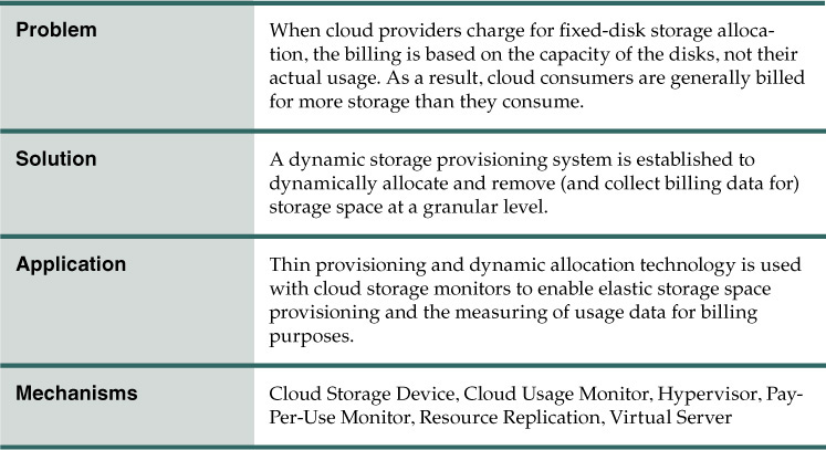
Problem
Cloud consumers are commonly charged for cloud-based storage space based on fixed-disk storage allocation. This means that they are charged based on the capacity of the fixed disks, regardless of their actual data storage consumption.
For example, a cloud consumer may provision a virtual server with the Windows Server operating system and three 150 GB hard drives. When the cloud consumer installs the operating system, it is billed for using 450 GBs of storage space, even though the operating system may only use 15 GBs.
The following steps are shown in Figure 3.18:
1. The cloud consumer requests a virtual server with three hard disks, each with a capacity of 150 GB.
2. The virtual server is provisioned via the Rapid Provisioning and Automated Administration patterns, with a total of 450 GB disk space.
3. The 450 GB of storage space is allocated to the virtual server by the cloud provider.
4. The cloud consumer has not installed any software yet, meaning the actual used space is currently 0 GB.
5. Because 450 GB has been allocated and reserved for the cloud consumer by the cloud provider, the cloud consumer will be charged for 450 GB of disk usage as of the point of allocation.

Solution
A system of dynamic storage provisioning is established so that the cloud consumer is billed, on a granular level, for the exact amount of storage that was actually used at any given time. This system uses thin provisioning technology for the dynamic allocation of storage space and is further supported by runtime usage monitoring to collect accurate usage data for billing purposes.
The following steps are shown in Figure 3.19:
1. The cloud consumer requests a virtual server with three hard disks, each with a capacity of 150 GB.
2. The virtual server is provisioned via the Rapid Provisioning and Automated Administration patterns, with a total of 450 GB disk space.
3. 450 GB of disk space is set as the maximum allowed disk usage for this virtual server, but no physical disk space has actually been reserved or allocated yet.
4. The cloud consumer has not installed any software yet, meaning the actual used space is currently 0 GB.
5. Because the allocated disk space is equal to the actual used space (which is currently at zero), the cloud consumer is not charged for any disk space usage.

The cloud consumer will only be charged when the disk space has actually been used.
Application
Thin provisioning software is installed on servers that need to process dynamic storage allocation. A specialized cloud usage monitor is employed to track and report actual disk usage.
The following steps are shown in Figure 3.20:
1. A request is received from the cloud consumer and the provisioning for a new virtual server instance begins.
2. As part of the provisioning process, the hard disks are chosen as dynamic or thin provisioned disks.
3. The hypervisor calls a dynamic disk allocation component to create thin disks for the virtual server.
4. Virtual server disks are created via the thin provisioning program and saved in a folder of near-zero size. The size of this folder and its files grows as operating applications are installed and additional files are copied onto the virtual server.
5. The pay-per-use monitor mechanism tracks the actual dynamically allocated storage for billing purposes.

Figure 3.20 A sample cloud architecture resulting from the application of the Elastic Disk Provisioning pattern.
Because the allocated space is equal to the amount of used space after applying the pattern, the cloud consumer will only be charged for 15 GB of storage usage. Should the cloud consumer later install an application that takes up 6 GB of disk space, it will be billed for using 21 GB from thereon.
Figure 3.21 provides an example of before and after the application of the Elastic Disk Provisioning pattern.

Figure 3.21 The fixed-disk allocation based provisioning model compared to the dynamic disk provisioning model.
Mechanisms
• Cloud Storage Device – This mechanism represents the cloud storage devices to which this pattern is primarily applied.
• Cloud Usage Monitor – Cloud usage monitors are used to track storage usage fluctuations in relation to the system established by this pattern.
• Hypervisor – The hypervisor is relied upon to perform built-in thin provisioning and to provision virtual servers with dynamic thin-disks in support of this pattern.
• Pay-Per-Use Monitor – The pay-per-use monitor is incorporated into the cloud architecture resulting from the application of this pattern in order to monitor and collect billing-related usage data as it corresponds to elastic provisioning.
• Resource Replication – Resource replication is part of an elastic disk provisioning system when conversion of dynamic thin-disk storage into static thick-disk storage is required.
• Virtual Server – The application of this pattern creates new instances of physical servers as virtual servers with dynamic disks.
Load Balanced Virtual Server Instances

How can a workload be balanced across virtual servers and their physical hosts?

Problem
When physical servers operate and are managed in isolation from one another, it is very challenging to keep cross-server workloads evenly balanced. One physical server can easily end up hosting more virtual servers or having to process greater workloads than neighboring physical servers (Figure 3.22).
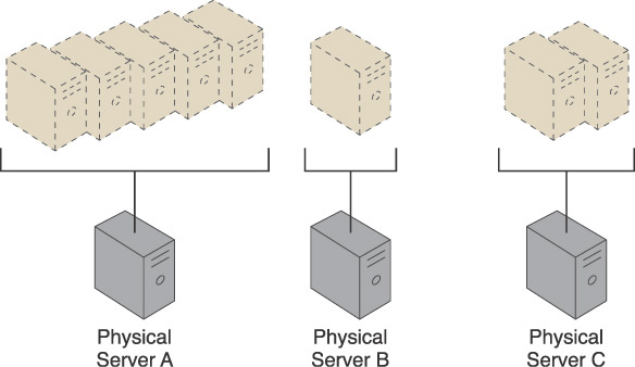
Figure 3.22 Three physical servers are encumbered with different quantities of virtual server instances, leading to both over-utilized and under-utilized IT resources.
Over time, the extent of over- and under-utilization of the physical servers can increase dramatically, leading to on-going performance challenges (for over-utilized servers) and constant waste (for the lost processing potential of under-utilized servers).
Solution
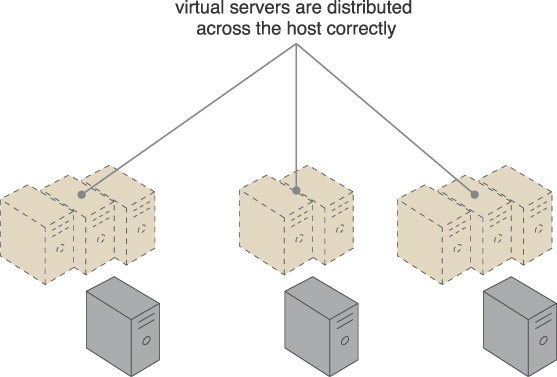
A capacity watchdog system is established to dynamically calculate virtual server instances and associated workloads and to correspondingly distribute the processing across available physical server hosts (Figure 3.23).
Application
The capacity watchdog system is comprised of a capacity watchdog cloud usage monitor, the live VM migration program, and a capacity planner. The capacity watchdog monitor keeps track of physical and virtual server usage and reports any significant fluctuations to the capacity planner, which is responsible for dynamically calculating physical server computing capacities against virtual server capacity requirements. The capacity planner can decide to move a virtual server to another host to distribute the workload at which point it signals the live VM migration program to perform the move of the targeted virtual server from one physical host to another.
The following steps are shown in Figures 3.24 to 3.26:
1. The Hypervisor Clustering pattern is applied to create a cluster of physical servers.
2. Policies and thresholds are defined for the capacity watchdog monitor.
3. The capacity watchdog monitors physical server capacities and virtual server processing.
4. The capacity watchdog monitor reports an over-utilization to the VIM.
5. The VIM signals the load balancer to redistribute the workload based on pre-defined thresholds.
6. The load balancer initiates live VM migration to move the virtual servers.
7. Live VM migration transitions the selected virtual servers from one physical host to another.
8. The workload is balanced across the physical servers in the cluster.
9. The capacity watchdog continues to monitor the workload and resource consumption.
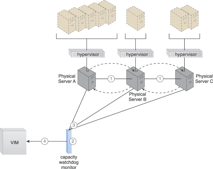
Figure 3.24 A cloud architecture scenario resulting from the application of the Load Balanced Virtual Server Instances pattern (Part I).

Figure 3.25 A cloud architecture scenario resulting from the application of the Load Balanced Virtual Server Instances pattern (Part II).
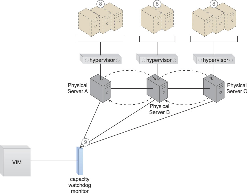
Figure 3.26 A cloud architecture scenario resulting from the application of the Load Balanced Virtual Server Instances pattern (Part III).
Mechanisms
• Automated Scaling Listener – The automated scaling listener may be incorporated into the system established by the application of this pattern to initiate the process of load balancing and to dynamically monitor workload coming to the virtual servers via the hypervisors.
• Cloud Storage Device – If virtual servers are not stored on a shared cloud storage device, this mechanism is used to copy virtual server folders from a cloud storage device that is accessible to the source hypervisor to another cloud storage device that is accessible to the destination hypervisor.
• Cloud Usage Monitor – Various cloud usage monitors, including the aforementioned capacity watchdog monitor, may be involved with collecting and processing physical server and virtual server usage information.
• Hypervisor – Hypervisors host the virtual servers that are migrated, as required, and further form the cluster used as the backbone of the capacity watchdog system. They are used to host virtual servers and allocate computing capacity to the virtual servers. The total available and consumed computing capacity of each hypervisor is measured by the virtual infrastructure manager (VIM) to determine whether any hypervisor is being over-utilized and needs to have virtual servers moved to another hypervisor.
• Live VM Migration – This mechanism is used to seamlessly migrate virtual servers between hypervisors to distribute the workload.
• Load Balancer – The load balancer mechanism is responsible for distributing the workload of the virtual servers between the hypervisors.
• Logical Network Perimeter – A logical network perimeter ensures that the destination of a given relocated virtual server is in compliance with SLA and privacy regulations.
• Resource Cluster – This mechanism is used to form the underlying hypervisor cluster in support of live VM migration.
• Resource Replication – The replication of virtual server instances may be required as part of the load balancing functionality.
• Virtual CPU – This mechanism is used to allocate CPU capacity to virtual servers. The amount of virtual CPU consumed by each virtual server running on a hypervisor is used to identify how the virtual servers are utilizing the hypervisor’s CPU resources.
• Virtual Infrastructure Manager (VIM) – This mechanism is used to make all of the necessary configurations before broadcasting the configurations to the hypervisors.
• Virtual RAM – Virtual servers are allocated the required memory via the use of this mechanism, which helps to evaluate how virtual servers are utilizing the hypervisors’ physical memory.
• Virtual Server – This is the mechanism to which this pattern is primarily applied.
• Virtual Switch – This mechanism is used to establish connectivity for the virtual servers after migrating between hypervisors to ensure that they will be accessible by cloud consumers and resource administrators.
• Virtualization Monitor – This mechanism is used to monitor the workload against the thresholds defined by the system administrator, in order to identify when the hypervisors are being over-utilized and require workload balancing.
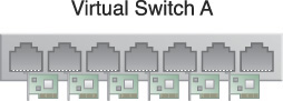
Load Balanced Virtual Switches

How can workloads be dynamically balanced on physical network connections to prevent bandwidth bottlenecks?
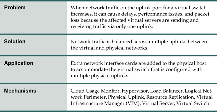
Problem
Virtual servers are connected to the outside world via virtual switches. When the network traffic on the uplink port increases, bandwidth bottlenecks can occur, resulting in transmission delays, performance issues, packet loss, and lag time because the virtual servers are sending and receiving traffic via the same uplink.
The following steps are shown in Figures 3.27 and 3.28:
1. A virtual switch has been created and is being used to interconnect virtual servers.
2. A physical network adapter has been attached to the virtual switch to be used as an uplink to the physical (external) network, connecting virtual servers to cloud consumers.
3. Cloud consumers can send their requests to virtual servers via the physical uplink. The virtual servers reply via the same uplink.
4. When the number of requests and responses increases, the amount of traffic passing through the physical uplink also grows. This further increases the number of packets that need to be processed and forwarded by the physical network adapter.
5. Because traffic increases beyond the physical adapter’s capacity, it is unable to handle the workload.
6. The network forms a bottleneck that results in performance degradation and the loss of delay-sensitive data packets.

Figure 3.27 A sequence of events that can lead to network bandwidth bottlenecking is shown (Part I).

Figure 3.28 A sequence of events that can lead to network bandwidth bottlenecking is shown (Part II).
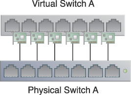
Solution
A load balancing system is established whereby multiple uplinks are provided to balance network traffic workloads.
Application
Balancing the network traffic load across multiple uplinks or redundant paths can help avoid slow transfers and data loss. Link aggregation can further be used to balance the traffic, thereby allowing the workload to be distributed across multiple uplinks at the same time. This way, none of the network cards are overloaded.
The following steps are shown in Figure 3.29:
1. Virtual servers are connected to the external network via a physical uplink, while actively responding to cloud consumer requests.
2. An increase in requests leads to increased network traffic, resulting in the physical uplink becoming a bottleneck.
3. Additional physical uplinks are added to enable network traffic to be distributed and balanced.
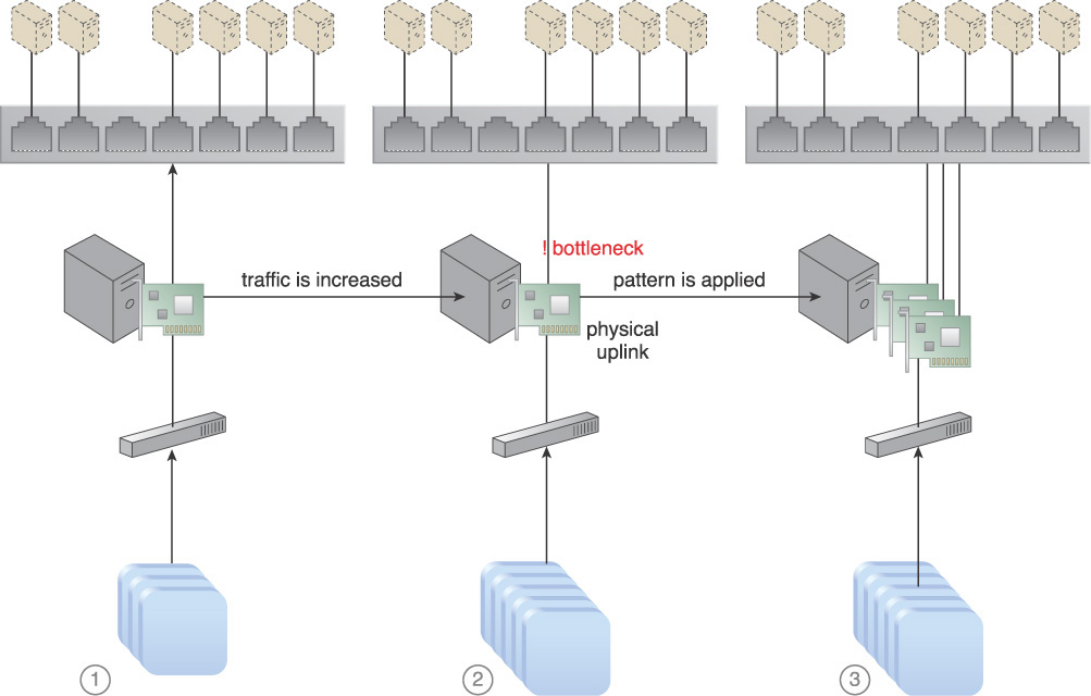
Figure 3.29 The addition of network interface cards and physical uplinks allows network workloads to be balanced.
The virtual switch needs to be configured to support multiple physical uplinks. The number of required uplinks can vary on a server-by-server basis. The uplinks generally need to be configured as a team (also known as an NIC team) for which traffic shaping policies are defined.
Mechanisms
• Cloud Usage Monitor – Cloud usage monitors may be employed to monitor network traffic and bandwidth usage.
• Hypervisor – Hypervisors host and provide the virtual servers with access to both the virtual switches and external network. They are responsible for both hosting virtual servers and forwarding the virtual servers’ network traffic across multiple physical uplinks to distribute the network load.
• Load Balancer – This mechanism supplies the runtime load balancing logic and performs the actual balancing of the network workload across the different uplinks.
• Logical Network Perimeter – The logical network perimeter can be used to create boundaries that protect and limit bandwidth usage for specific cloud consumers.
• Physical Uplink – The physical uplink mechanism is used to connect virtual switches to physical switches. The use of this mechanism enables each virtual switch to be connected to the physical network via two or more physical connections, for load-balancing purposes.
• Resource Replication – This mechanism is utilized to generate additional uplinks to the virtual switch.
• Virtual Infrastructure Manager (VIM) – This mechanism performs virtual switch configurations and attaches physical uplinks to the virtual switches.
• Virtual Server – Virtual servers host the IT resources that benefit from the additional uplinks and bandwidth via virtual switches.
• Virtual Switch – The virtual switch mechanism is used to connect virtual servers to the physical network and to cloud consumers.
Service State Management

How can stateful cloud services be optimized to minimize runtime IT resource consumption?

Problem
A cloud service may need to carry out functions that require prolonged processing across underlying IT resources or other cloud-based services that are invoked. While waiting for responses from IT resources or other cloud services, the primary cloud service may be unnecessarily consuming memory via the temporary storage of state data. The cloud service may also be storing RAM or CPU data, which represents memory consumed by the virtual server instance itself.
While retaining state data in-memory, the cloud service is considered to be in a stateful condition. When stateful, the cloud service is actively consuming infrastructure-level resources that could otherwise be shared within the cloud. Furthermore, the cloud consumer may be charged usage fees for the on-going consumption of these resources.
Solution
The cloud service architecture is designed to incorporate the use of the state management database mechanism, a specialized repository used for the temporary deferral of state data. This solution applies to custom cloud services that automate business tasks, as well as cloud service products (such as those based on cloud delivery models) offered by cloud providers.
Application
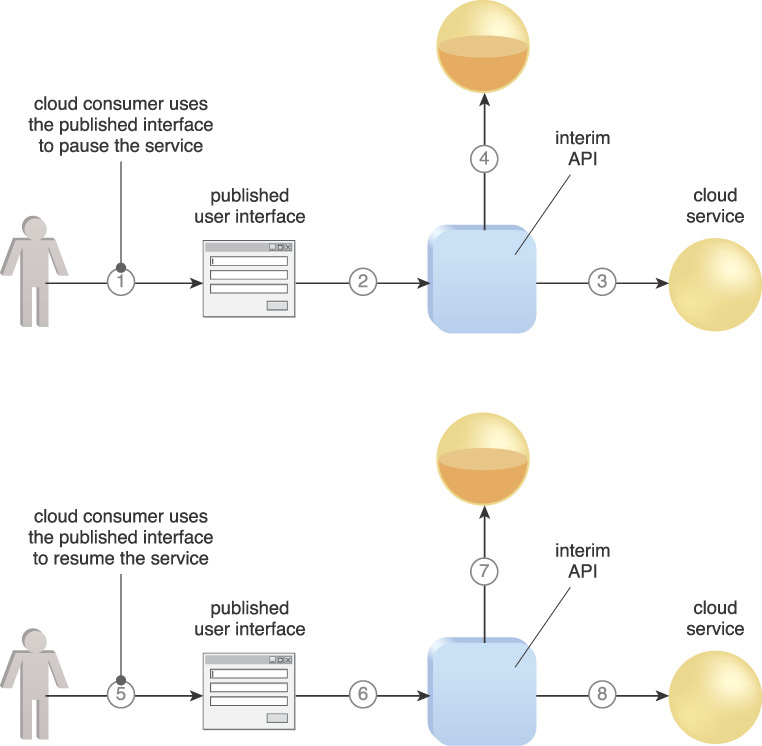
State information can be programmatically deferred by executing conditional logic within the cloud service, or it can be manually deferred by a cloud resource administrator using a usage and administration portal.
The following steps are shown in Figure 3.30:
1. The cloud consumer uses the usage and administration portal to request that the cloud service status be paused and deferred.
2. The request is forwarded to an API-enabled system that interacts with the state management database mechanism.
3. The system reads the service status.
4. The system saves it to the state management database.
5. The cloud consumer requests that the service be reactivated via the usage and administration portal.
6. The cloud consumer request is forwarded to the system.
7. The system interacts with the state management database to retrieve the status of the cloud service.
8. The cloud service status is restored and cloud service activity resumes.
Note that resuming a paused cloud service may trigger a resource constraint, depending on how long the state data was deferred and how the IT resources required by the stateful cloud service are managed while the cloud service is stateless.
Mechanisms
• Cloud Storage Device – This mechanism is used in the same way as the state management database in relation to this pattern.
• Cloud Usage Monitor – Specialized cloud usage monitors may be employed for proactive monitoring of IT resource processing and server memory usage.
• Hypervisor – In some cases, state management database functionality is provided at the hypervisor level.
• Pay-Per-Use Monitor – This monitoring mechanism collects granular resource usage data for state data held in memory, as well as granular storage usage data for when state data is temporarily stored in a cloud storage device.
• Resource Replication – Resource replication is used to instantiate new instances of IT resources that may need to be deactivated and re-activated as part of state management deferral logic.
• State Management Database – This is the core mechanism used to implement a state management architecture.
• Virtual Server – This mechanism generally hosts the state management database and is responsible for providing the processing features used to transfer state data to and from the database.
Storage Workload Management

How can storage processing workloads be dynamically distributed across multiple storage devices?
Problem
When cloud storage devices are utilized independently, the changes resulting from some devices being over-utilized while others remain under-utilized are significant. Over-utilized storage devices increase the workload on the storage controller and can cause a range of performance challenges (Figure 3.31). Under-utilized storage devices may be wasteful due to lost processing and storage capacity potential.
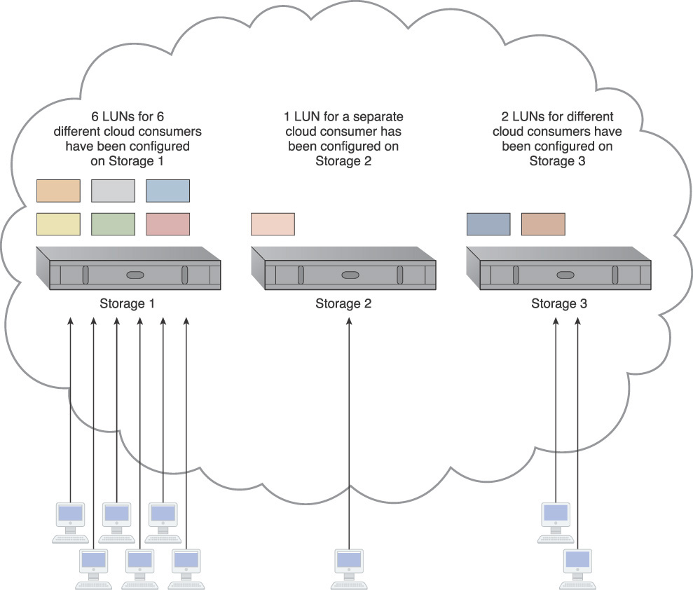
Figure 3.31 An imbalanced cloud storage architecture where six storage LUNs are located on Storage 1 for use by different cloud consumers, while Storage 2 and Storage 3 each host one and two additional LUNs respectively. Because it hosts the most LUNs, the majority of the workload ends up with Storage 1.
Solution
The LUNs are evenly distributed across available cloud storage devices and a storage capacity system is established to ensure that runtime workloads are evenly distributed across the LUNs (Figure 3.32).
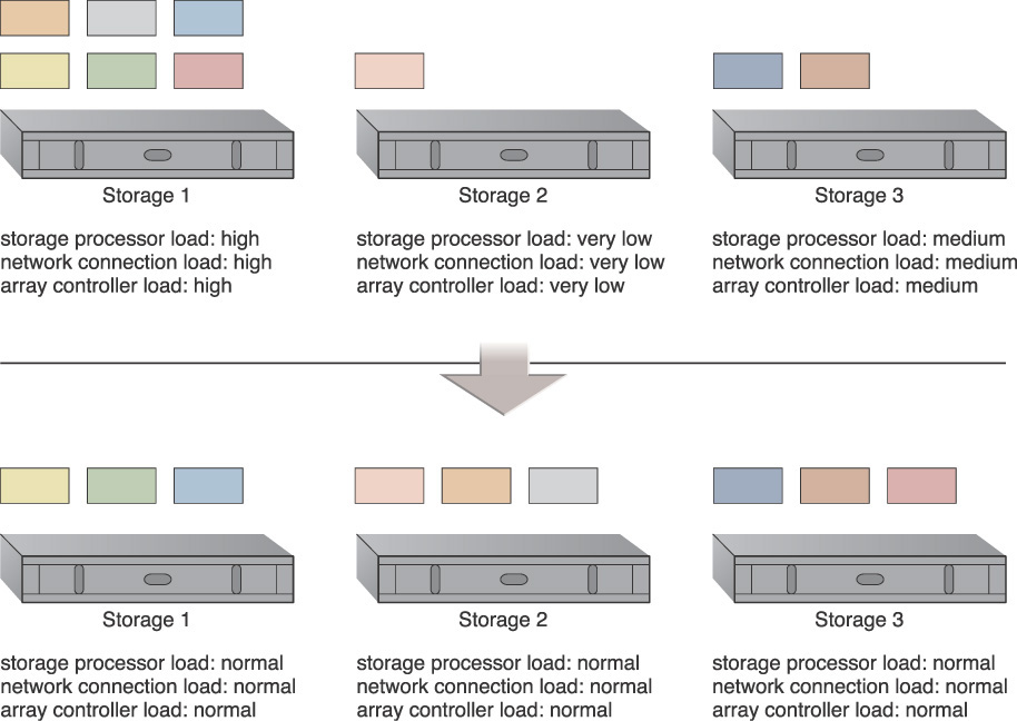
Figure 3.32 LUNs are dynamically distributed across cloud storage devices, resulting in more even distribution of associated types of workloads.
Application
Combining the different storage devices as a group allows LUN data to be spread out equally among available storage hosts. A storage management station is configured and an automated scaling listener is positioned to monitor and equalize runtime workloads among the storage devices in the group.
The following steps are shown in Figures 3.33 to 3.35:
1. The storage capacity system and the storage capacity monitor are configured to survey three storage devices in realtime. As part of this configuration, some workload and capacity thresholds are defined.
2. The storage capacity monitor determines that the workload on Storage 1 is reaching a predefined threshold.
3. The storage capacity monitor informs the storage capacity system that Storage 1 is over-utilized.
4. The storage capacity system initiates workload balancing via the storage load/capacity manager (not shown).
5. The storage load/capacity manager calls for LUN migration to move some of the storage LUNs from Storage 1 to the other two storage devices.
6. LUN migration transitions the LUNs.

Figure 3.33 A cloud architecture resulting from the application of the Storage Workload Management pattern (Part I).
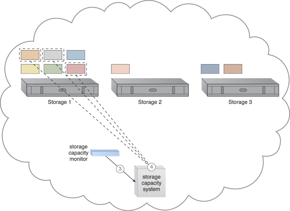
Figure 3.34 A cloud architecture resulting from the application of the Storage Workload Management pattern (Part II).
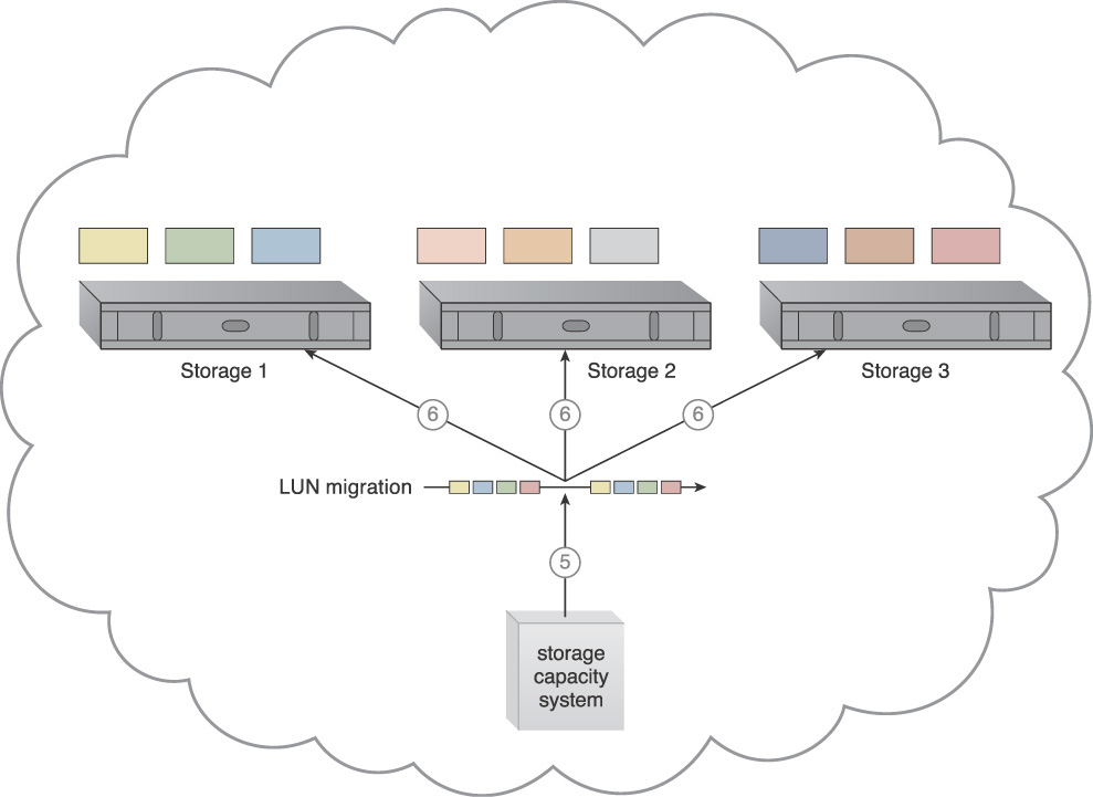
Figure 3.35 A cloud architecture resulting from the application of the Storage Workload Management pattern (Part III).
Note that if some of the LUNs are being accessed less frequently or only at specific times, the storage capacity system can keep the hosting storage device in power-saving mode until it is needed.
Mechanisms
• Audit Monitor – This monitoring mechanism may need to be involved because the system established by this pattern can physically relocate data, perhaps even to other geographical regions.
• Automated Scaling Listener – The automated scaling listener may be incorporated to observe and respond to workload fluctuations.
• Cloud Storage Device – This is the primary mechanism to which this pattern is applied.
• Cloud Usage Monitor – In addition to the capacity workload monitor, other types of cloud usage monitors may be deployed to track LUN movements and collect workload distribution statistics.
• Load Balancer – This mechanism can be added to horizontally balance workloads across available cloud storage devices.
• Logical Network Perimeter – This mechanism provides a level of isolation to ensure that cloud consumer data that is relocated to a new location remains inaccessible to unauthorized cloud consumers.
Dynamic Data Normalization
How can redundant data within cloud storage devices be automatically avoided?

Problem
Redundant data can cause a range of issues in cloud environments, such as:
• Increased time required to store and catalog files
• Increased required storage and backup space
• Increased costs due to increased data volume
• Increased time required for replication to secondary storage
• Increased time required to backup data
For example, a cloud consumer copies 100 MB of files onto a cloud storage device. If it copies the data redundantly, ten times, the consequences can be considerable:
• The cloud consumer will be charged for using 1,000 MBs (1 GB) of storage space even though it is only storing 100 MBs of unique data.
• The cloud provider needs to provide an unnecessary 900 megabytes of space on both the online cloud storage device and any backup storage systems (such as tape drives).
• It takes nine times the amount of time required to store and catalog data.
• If the cloud provider is performing a site recovery, the data replication duration and performance will suffer, since 1,000 MBs need to be replicated instead of 100 MBs.
In multitenant public clouds, these impacts can be significantly amplified.
Solution
A data de-duplication system is established to prevent cloud consumers from inadvertently saving redundant copies of data. This system detects and eliminates exact amounts of redundant data on cloud storage devices, and can be applied to both block and file-based storage devices (although it works most effectively on the former). The data de-duplication system checks each block it receives to determine whether it is redundant with a block that has already been received. Redundant blocks are replaced with pointers to the equivalent blocks that are already stored.
Application
A de-duplication system examines received data prior to passing it to storage controllers (Figure 3.36). As part of the examination process, it assigns a hash code to every piece of data that has been processed and stored. It also keeps an index of hashes and pieces. As a result, if a new block of data is received, its generated hash is compared with the current stored hashes to decide if it is a new or duplicate block of data.
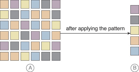
Figure 3.36 In Part A, datasets containing redundant data unnecessarily bloat data storage. The Dynamic Data Normalization pattern results in the constant and automatic streamlining of data as shown in Part B, regardless of how denormalized the data received from the cloud consumer is.
If it is a new block, it is saved. If the data is a duplicate, it is eliminated and a link (or pointer) to the original data block is created and saved in the cloud storage device. If a request for the data block is received at a later point, the pointer forwards the request to the original data block.
This pattern can be applied to both disk storage and backup tape drives. A cloud provider may decide to prevent redundant data only on backup cloud storage devices, while others may more aggressively implement the data de-duplication system on all cloud storage devices.
There are different methods and algorithms for comparing blocks of data and deciding whether they are duplications of other blocks.
Mechanisms
• Cloud Storage Device – This mechanism represents the cloud storage devices to which this pattern is primarily applied in relation to the normalization of both existing and newly added data.
Cross-Storage Device Vertical Tiering

How can the vertical scaling of data processing be carried out dynamically?

Problem
After working with a provisioned cloud storage device, a cloud consumer may determine that the device is unable to accommodate its necessary performance requirements. Conventional approaches to vertically scaling the cloud storage device include adding more bandwidth to increase IOPS (input/output per second) and adding more data processing power. This type of vertical scaling can be inefficient and time consuming to implement, and can result in waste when the increased capacity is no longer needed.
This approach is depicted in the following scenario in which a number of requests for access to a red LUN increased, requiring it to be manually moved to a high performance storage device.
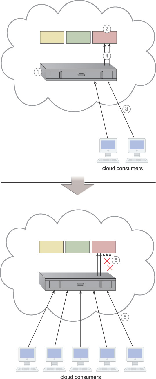
The following steps are shown in Figure 3.37:
1. The cloud provider installs and configures a storage device.
2. The cloud provider creates the required LUNs for the cloud consumers.
3. Storage LUNs are presented to their respective cloud consumers, who begin using them.
4. The storage devices start forwarding requests to cloud consumer LUNs.
5. The number of requests increases significantly, resulting in high storage bandwidth and performance demands.
6. Some of the requests are rejected or time out due to performance capacity limitations.
Solution
A system is established that can survive bandwidth and data processing power constraints (thereby preventing timeouts) and that introduces vertical scaling between different storage devices possessing different capacities. As a result, LUNs can automatically scale up and down across multiple devices, allowing requests to use the appropriate level of storage devices to perform the tasks required by the cloud consumer.
Application
Although the automated tiering technology can move data to cloud storage devices with the same storage processing capacity, the new cloud storage devices with increased capacity need to be made available. For example, solid-state drives (SSDs) may be suitable devices for upgrading data processing power.
The automated scaling listener monitors requests sent to specific LUNs. When it identifies that a predefined threshold is reached, it signals the storage management program to move the LUN to a higher capacity device. Interruption is prevented because a disconnection during the transfer never occurs. While the LUN data is scaling up to another device, its original device remains up and running. As soon as the scaling is completed, cloud consumer requests are automatically redirected to the new cloud storage device.
The following steps are shown in Figures 3.38 to 3.40:
1. The primary storage (also known as the “lower capacity storage”) is installed and configured, and responding to cloud consumer storage requests.
2. A secondary storage device with higher capacity and performance is installed.
3. The LUN migration is configured via a storage management program.
4. Thresholds are defined in the automated scaling listener, which monitors the requests.
5. The storage management program is installed and configured to categorize the storage based on device performance.
6. Cloud consumer requests are sent to the (lower capacity) primary storage device.
7. The number of cloud consumer requests reaches the predefined request threshold.
8. The automated scaling listener signals the storage management program that scaling is required.
9. The storage management program calls the LUN migration program to move the cloud consumer’s red LUN to a higher capacity storage device.
10. The LUN migration program initiates the move of the red LUN to a higher capacity storage device.
11. Even though the LUN was moved to a new storage device, cloud consumer requests are still being sent to the original storage device.
12. The storage service gateway forwards the cloud consumer storage requests from the red LUN to the new storage device.
13. The red LUN is deleted from the lower capacity device (via the storage management and LUN migration programs).
14. The automated scaling listener monitors the cloud consumer requests for access to the higher capacity storage for the red LUN.
15. Usage and billing data is tracked and stored via the pay-per-use monitor mechanism.
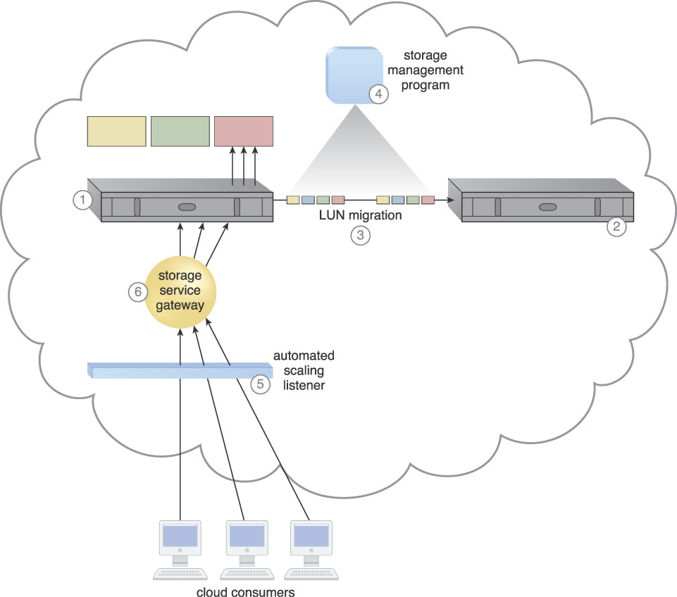
Figure 3.38 A cloud architecture resulting from the application of the Cross-Storage Device Vertical Tiering pattern (Part I).
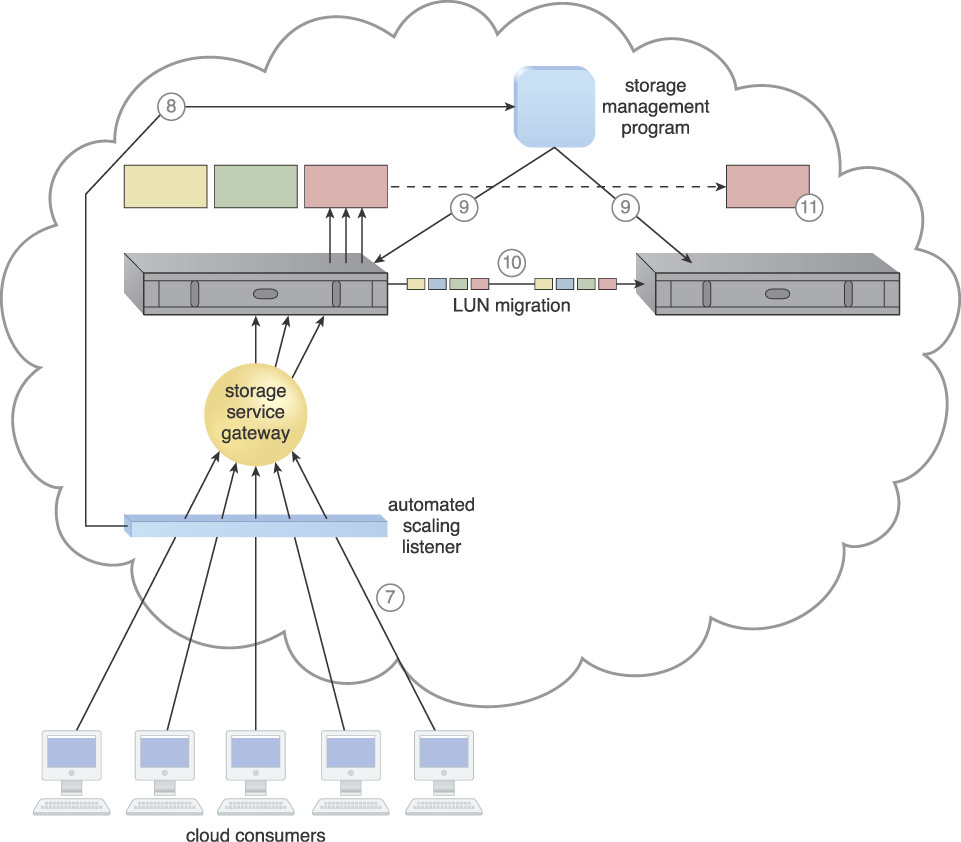
Figure 3.39 A cloud architecture resulting from the application of the Cross-Storage Device Vertical Tiering pattern (Part II).
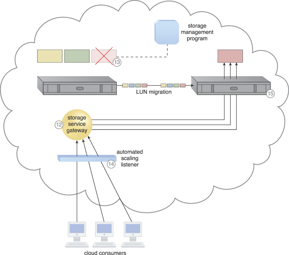
Figure 3.40 A cloud architecture resulting from the application of the Cross-Storage Device Vertical Tiering pattern (Part III).
Mechanisms
• Audit Monitor – This mechanism ensures that the relocation of cloud consumer data via the application of this pattern does not conflict with any legal or data privacy regulations or policies.
• Automated Scaling Listener – The automated scaling listener monitors the traffic from the cloud consumer to the storage device, and initiates the data transfer process across storage devices.
• Cloud Storage Device – This mechanism represents the cloud storage devices that are affected by the application of this pattern.
• Cloud Usage Monitor – This infrastructure mechanism represents various runtime monitoring requirements for tracking and recording the cloud consumer data transfer and usage at both source and destination storage locations.
• Pay-Per-Use Monitor – Within the context of this pattern, the pay-per-use monitor collects storage usage information on source and destination storage locations, as well as resource usage information for carrying out the cross-storage tiering functionality.
Intra-Storage Device Vertical Data Tiering

How can the dynamic vertical scaling of data be carried out within a storage device?

Problem
When a cloud consumer has a firm requirement to limit the storage of data to a single cloud storage device, the capacity of that device to store and process data can become a source of performance-related challenges. For example, different servers, applications, and cloud services that are forced to use the same device may have data access and I/O requirements that are incompatible with the cloud storage device’s capabilities.
Solution
A system is established to support vertical scaling within a single cloud storage device (Figure 3.41). This intra-device scaling system utilizes the availability of different disk types with different capacities.
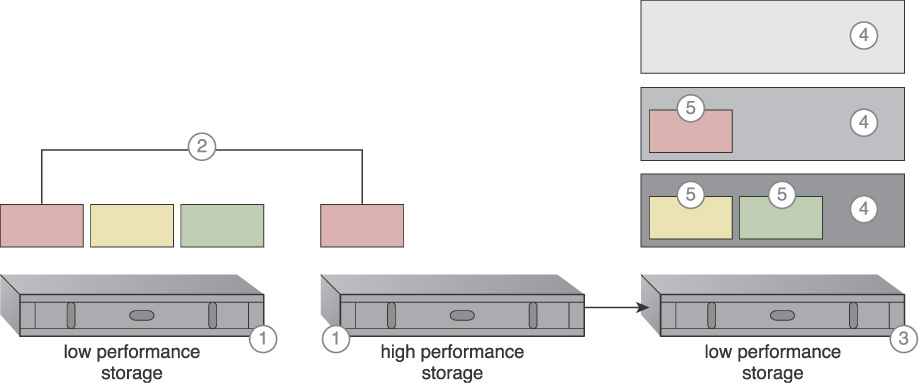
Figure 3.41 A conventional horizontal scaling system involving two cloud storage devices (1, 2) is transitioned to an intra-storage device system (3) capable of vertically scaling through disk types graded into different tiers (4). Each LUN is moved to a tier that corresponds to its processing and storage requirements (5).
Application
The cloud storage architecture requires the use of a complex storage device that supports different types of hard disks, in particular high-performance disks, such as SATAs, SASs, and SSDs. The disk types are organized into graded tiers, so that LUN migration can vertically scale the device based on the allocation of disk types that align to the processing and capacity requirements at hand.
After disk categorization, data load conditions and definitions are set so that the LUNs are able to either move to a higher or lower grade depending on when pre-defined conditions are met. These thresholds and conditions are used by the automated scaling listener when monitoring runtime data processing traffic.
The following steps are shown in Figures 3.42 to 3.44:
1. A storage device that supports different types of hard disks is installed.
2. Different types of hard disks are installed in the enclosures.
3. Similar disk types are grouped together to create different grades of disk groups based on their I/O performance.
4. Two LUNs have been created on Disk Group 1: LUN red and LUN yellow.
5. The automated scaling listener monitors the requests and compares them with the predefined thresholds.
6. The usage monitor tracks the actual amount of disk usage on the red LUN based on free space and disk group performance.
7. The automated scaling listener realizes that the number of requests coming to the red LUN is reaching the predefined threshold, and the red LUN needs to be moved to a higher performance disk group, and informs the storage management program.
8. The storage management program signals the LUN migration to move the red LUN to a higher performance disk group.
9. The LUN migration works with the storage controller to move the red LUN to the higher capacity disk group.
10. The red LUN is moved to a higher performance disk group.
11. The usage monitor is still performing the same task of monitoring the disk usage. However, the difference is that the service price of the red LUN will be higher than before because it is using a higher performance disk group.
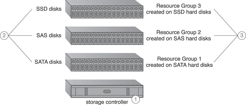
Figure 3.42 An intra-device cloud storage architecture resulting from the application of this pattern (Part I).
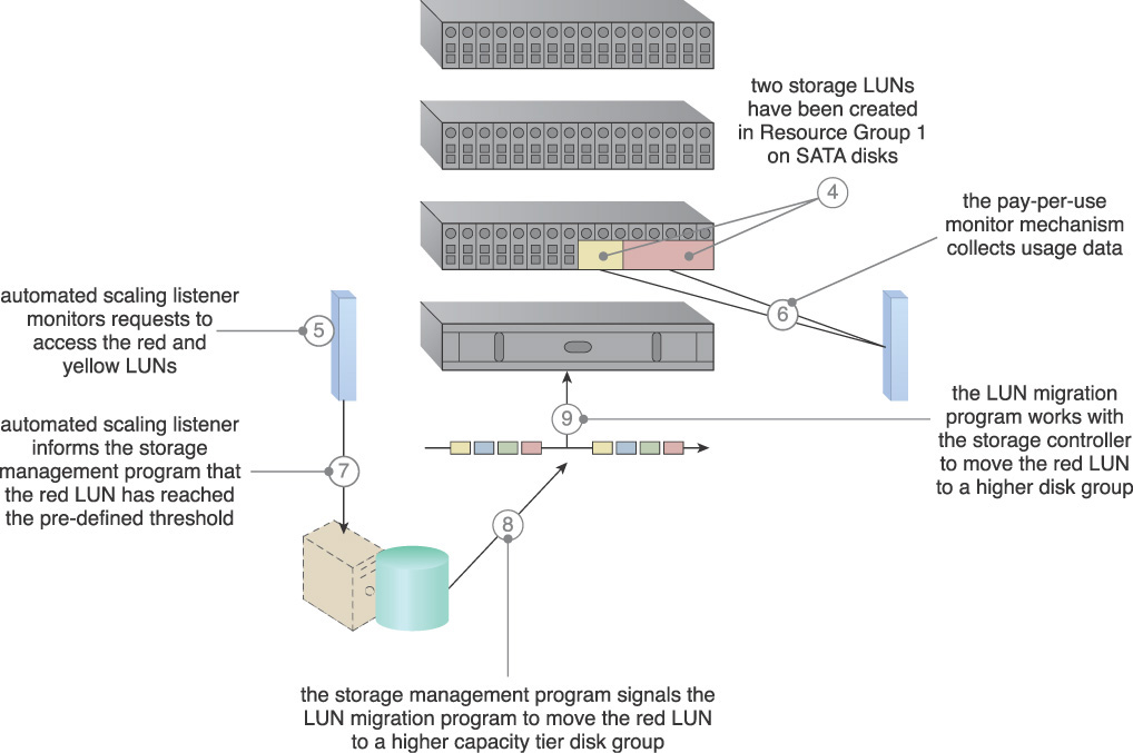
Figure 3.43 An intra-device cloud storage architecture resulting from the application of this pattern (Part II).
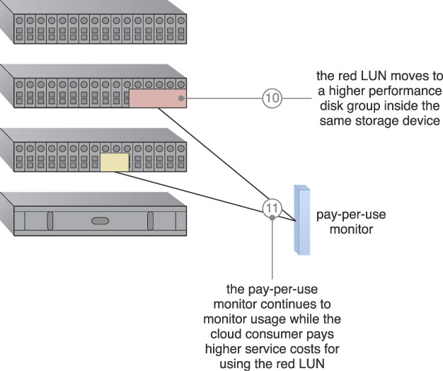
Figure 3.44 An intra-device cloud storage architecture resulting from the application of this pattern (Part III).
Mechanisms
• Automated Scaling Listener – The automated scaling listener monitors and compares the cloud storage device’s workload with predefined thresholds, so that data can be distributed between disk type tiers, as per workload fluctuations.
• Cloud Storage Device – This is the mechanism to which this pattern is primarily applied.
• Cloud Usage Monitor – Various cloud usage monitors may be involved with the collection and logging of disk usage information pertaining to the storage device and its individual disk type tiers.
• Pay-Per-Use Monitor – This mechanism actively monitors and collects billing-related usage data in response to vertical scaling activity.
Memory Over-Committing

How can multiple virtual servers be hosted on a single host when the virtual servers’ aggregate memory exceeds the physical memory that is available on the host?

Problem
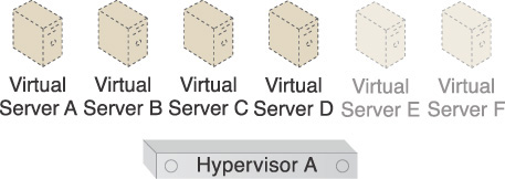
Virtualization supports server consolidation, which is the hosting of multiple virtual servers on the same host or the physical server that is running the hypervisor. In the following example in Figure 3.45, six virtual servers are shown. Two virtual servers with 8 GBs each, two virtual servers with 4 GBs each, and two virtual servers with 2 GBs each have been defined. The virtual servers need a total of 44 GBs of memory.

Figure 3.45 The virtual servers require a total of 44 GBs of memory to be hosted on the same hypervisor.
The virtual servers cannot be run if the host only has 32 GBs of physical memory available, which is less than the memory required by the virtual servers. Figure 3.46 illustrates a situation in which some of the virtual servers cannot be hosted or powered on by the same host as a result.
The system cannot power on the remaining virtual servers when the amount of allocated memory reaches 32 GBs, because it has run out of memory.
Solution
Memory virtualization is implemented to enable more virtual servers to be hosted on the same host by allowing its physical memory to be exceeded by the total memory configuration of the virtual servers that require hosting (Figure 3.47).

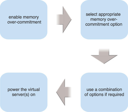
Application
Figure 3.48 illustrates the steps that need to be applied. All of the virtual servers can be powered on after memory over-commitment is applied. The host is allowed to allocate an amount of memory that is greater than the amount of available physical memory.
Note that if Resource Reservation (106) needs to be applied to reserve a specific amount of memory for a virtual server, that amount will be deducted from the physical memory of the host and directly allocated to that virtual server. For example, if the host in Figure 3.49 has 32 GBs of memory and a virtual server has reserved 8 GBs, the amount of memory that remains available for the rest of the virtual servers is 24 GBs.

If an unsuitable memory over-committing technique is used and the over-committing limit is violated, then the host may end up not having sufficient memory. In this case, the host will have to swap to disk by using swap memory, which can have a significant performance impact on memory-intensive applications.
Mechanisms
• Hypervisor – The hypervisor mechanism is used to host virtual servers, and provides techniques and features for sharing and partitioning physical memory between multiple virtual servers for concurrent usage.
• Virtual Infrastructure Manager (VIM) – This mechanism establishes features for monitoring and analyzing the memory consumption and utilization status of hypervisors and virtual servers.
• Virtual RAM – Physical memory is partitioned and allocated to virtual servers in the form of virtual memory. This mechanism provides the virtual servers with access to the physical memory under the control of the hypervisor.
• Virtualization Agent – This mechanism provides techniques for improving memory utilization, and helps indicate to a given hypervisor which memory pages can be reclaimed from virtual servers if the hypervisor needs to free up physical memory.
• Virtualization Monitor – This mechanism establishes the tools and techniques required to actively monitor memory consumption, and send alerts and notifications whenever utilization thresholds are being met.
NIC Teaming

How can the capacity of multiple NICs be combined for virtual servers to use while improving availability?
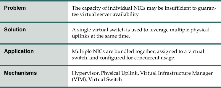
Problem
The boot availability and capacity of a single physical uplink may sometimes be inadequate for the virtual switch.
In the following example, the virtual switch has two physical uplinks. Only one is active while the other is in standby mode. As illustrated in Figure 3.50, this arrangement does not provide sufficient availability or capacity, since only one physical uplink’s capacity is in use at any one time.

Figure 3.50 Virtual Switch A has two physical uplinks named Physical Uplinks A and B. Physical Uplink B is not active.
Solution
The capacity of multiple physical NICs needs to be combined so that their aggregated bandwidth can be available to keep the remaining NICs operational if one of the NICs goes down (Figure 3.51). NIC teaming is a feature that allows physical NICs to be bundled together to form a logical port. This can be used for:
• Redundancy/High Availability – When a virtual switch uses a teamed NIC network to connect to a physical network, traffic is sent via other available NICs should one of the physical NICs fail.
• Load Balancing – When a switch has uplinks consisting of multiple NICs, it can send traffic via all of the uplinks simultaneously to reduce congestion and to balance the workload and traffic.
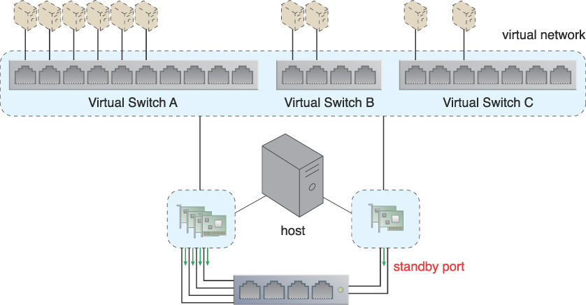
Figure 3.51 The physical NICs assigned to Virtual Switch A act as a team and simultaneously forward packets to balance the load. However, one of the two NICs that are teamed up for Virtual Switch C is not required to simultaneously forward traffic from both NICs. Instead, that NIC has been configured as a standby NIC. It will take over the forwarding of the packets to maintain redundancy and high availability, should anything happen to the original NIC.
Application
In Figure 3.52, multiple physical uplinks are added to the virtual switch. Figure 3.53 illustrates the connecting of the physical uplinks to the physical switch.
A NIC team is defined using a teaming policy, either via the VIM server or directly on the hypervisor. The physical switch needs to be configured in such a way that none of the physical uplinks are blocked. Implementing a teaming policy ensures that all of the physical uplinks remain active and that the aggregated bandwidth capacity is available for the virtual switch to use. If one of the physical uplinks fails or becomes disconnected, the other uplinks can remain operational to continue sending packets.
Applying this pattern increases the amount of uplink bandwidth available for the virtual switch while improving redundancy and availability. However, this pattern uses the physical NICs exclusively, meaning they cannot be used for anything else.
Mechanisms
• Hypervisor – This mechanism enables the creation of virtual servers and virtual switches, and also provides features that allow physical NICs installed on a physical server to be attached to virtual switches.
• Physical Uplink – This mechanism connects virtual switches to the physical network, and enables virtual servers to use the virtual switches to communicate with the physical network.
• Virtual Infrastructure Manager (VIM) – This mechanism is used to create and manage virtual switches and attach physical uplinks to virtual switches. The VIM also dictates configuration and utilization policies to hypervisors on how to utilize the physical uplinks.
• Virtual Switch – This mechanism is used to establish connectivity between virtual servers and the physical network, via the physical uplinks that are attached to the virtual switches.
Broad Access
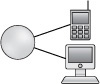
How can cloud services be made accessible to a diverse range of cloud service consumers?
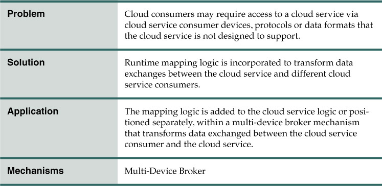
Problem
Cloud service implementations are commonly designed to support one type of cloud service consumer. However, different cloud consumers may need or prefer to access a given cloud service using different cloud service consumer devices, such as mobile devices, Web browsers, or proprietary user interfaces. Limiting the types of cloud service consumers and devices that a cloud service can support reduces its overall reuse and utilization potential.
Solution
Runtime mapping logic is incorporated into the cloud service architecture to support APIs for multiple types of cloud service consumer devices (Figure 3.54). Transport protocols, messaging protocols, data models, and other types of data sent to the cloud service are transformed at runtime into formats supported by the cloud service’s native logic.
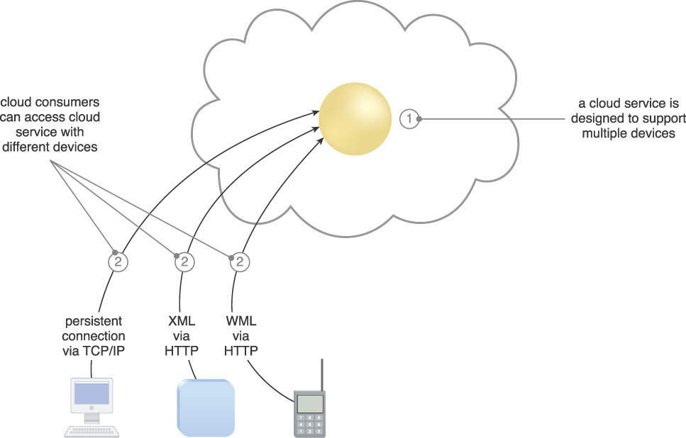
Figure 3.54 A cloud service containing runtime mapping logic is implemented (1) and made available to different kinds of cloud service consumer devices (2).
Application
The application of this pattern focuses on the creation and architectural placement of mapping logic. The multi-device broker is most commonly utilized as a component, separate from or within the cloud service architecture that houses the mapping logic (Figure 3.55). Some multi-device brokers can act as a gateway on behalf of multiple cloud services, thereby establishing themselves as the point of contact for cloud service consumers. Other multi-device brokers are positioned as service agents to transparently intercept messages upon which the mapping logic is carried out at runtime.

Figure 3.55 The cloud consumer (top) accesses and configures a physical server using a standard device and protocol that is now supported as a result of applying the Broad Access pattern. The cloud consumer (bottom) later accesses the cloud environment again to install a virtual server on the same physical server, and deploys an operating system and a database server. Both actions represent management tasks that can be accomplished via different devices brokered by the same centralized multi-device broker mechanism.
Alternatively, the mapping logic can be built right into the cloud service architecture by becoming an extension of the cloud service logic. A façade can be added to separate this logic as an independent component within the cloud service implementation.