

Storage Essentials
In this chapter, you will learn how to
• Explain how drive storage systems work
• Describe the types of disk interfaces and their characteristics
• Combine multiple disks to achieve larger storage and fault tolerance
• Classify the way hosts interact with disks
At its most basic level, storage starts with a disk. These disks, connected either internally or externally to systems via interfaces, can be accessed by systems to read or write data. Disks can also be combined to achieve greater speed than each disk could individually provide, or they can be combined to protect against one or more disk failures. One or more disks are then presented to a host, enabling it and its applications to work with the storage.
How Disk Storage Systems Work
The hard disk drive (HDD) or hard drive is a good place to begin a discussion on storage. HDDs have been in use in computer systems for decades, and the principles behind their basic operation remain largely unchanged. The solid-state drive (SSD) is a more recent introduction, and although it uses different principles for storing data, it has not replaced the HDD. SSD and HDD both have their uses in storage systems today, which will be explained in this section.
Physical Components
Originally, the term hard disk drive was used to differentiate the rigid, inflexible metal drive from floppy disks, which could be easily bent. While floppy disks are mostly a thing of the past, the hard disk drive term remains. HDDs are physically composed of platters, heads, a spindle, and an actuator arm all sealed within a rectangular container that is 3.5 or 2.5 inches wide called the head disk assembly (HDA). This is pictured in Figure 1-1. Higher capacity can be obtained from 3.5-inch drives because they have a larger surface area. These 3.5-inch drives are typically installed in desktops and servers, while 2.5-inch drives are commonly found in laptops. Some servers use 2.5-inch drives in cases where an increased number of drives is preferred over increased capacity. Beginning with the platter, each of these components is discussed in more detail, and key performance metrics are introduced for several components.
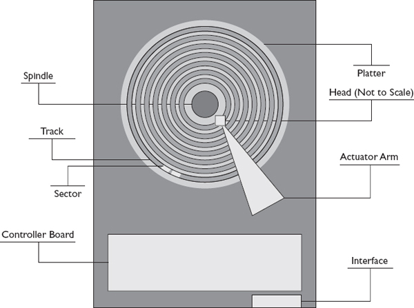
Figure 1-1 HDD components
Platter
If you open an HDD, the first thing you notice is a stack of round flat surfaces known as platters. Platters are made of thin but rigid sheets of aluminum, glass, or ceramic. The platters are covered on both the top and the bottom with a thin coating of substrate filled with small bits of metal. The majority of drives contain two or three platters providing four or six usable surfaces for storing data.
Spindle
An HDD has multiple platters connected to a rod called a spindle. The spindle and all the platters are rotated at a consistent rate by the spindle motor. Spindles commonly spin at 7,200 or 10,000 or 15,000 rotations per minute (rpm). Disk rpm is the determining factor in the rotational latency, an important disk performance metric.
Rotational latency is the amount of time it takes to move the platter to the desired location, measured in milliseconds (ms). Full rotational latency is the amount of time it takes to turn the platter 360 degrees. Average rotational latency is roughly half the full rotational latency. Average rotational latency is a significant metric in determining the time it takes to read random data. Rotational latency is directly related to rotational speed, with faster disks (higher rpm) providing lower rotational latency. Average rotational latency can be computed using the following formula:
Average rotational latency = 0.5 / (rpm/60) × 1000
With this formula, a disk with 10k (10,000) rpm would have a rotational latency of 3 ms.
Cylinder
HDDs are organized into a series of concentric rings similar to the rings on a tree. Each ring—called a cylinder—is numbered, starting at 0 with the outermost cylinder. Cylinders provide a precise location where data is located relative to the platter’s center. Each cylinder consists of sections from the platters located directly above and below it. These cylinder sections on each platter start and stop at the same relative location. The cylinder area on an individual platter is called a track, so cylinder 0 would comprise track 0 on the top and bottom of all platters in the disk. Figure 1-2 shows hard disk platters and the tracks that make up cylinder 0. A physical demarcation, delineating the tracks on the platter, enables the head (discussed next) to follow and remain in proper alignment.
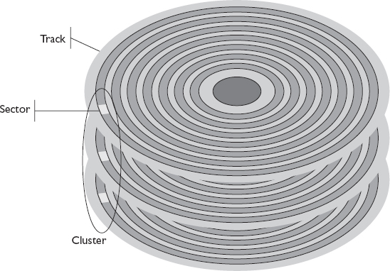
Figure 1-2 Cylinder 0 and the tracks comprising it
Tracks are organized into sectors, each of a fixed length. A process, often performed by the disk manufacturer, called low-level formatting creates the sectors on the disk and marks the areas before and after each sector with an ID, making them ready for use. These sectors make it easier to more precisely locate data on the disk, and they are more manageable because of their consistent size. Disks used a sector size of 512 bytes until 2009, when advanced format drives were released that use 4,096 bytes, or 4 kilobytes (4KB), per sector. Advanced format drives are the most common ones in use today.
Earlier HDD designs stored the same amount of data on each track even though the inner tracks were much smaller physically than the outer tracks. Later designs incorporated zone bit recording to divide the tracks into zones, with some zones having more sectors than others. Each track in a zone has the same number of sectors in it, with the zone closest to the center having the fewest sectors. In this way, more data could be written to the outside tracks to make use of much more space on the platters. However, with zone bit recording, the disk still spins at a constant rate, so the data stored on the outside zones is read much quicker than data on inside zones. Since performance is partially determined by where benchmarking data is stored, this can lead to inconsistent results. A better result can be achieved when the benchmark is performed on the outer zones for all disks that need to be compared.
Head
HDDs contain small electromagnets called heads. These heads, one for both the top and bottom sides of each platter in the disk, are attached to an actuator arm. All heads are attached to the same actuator arm, so they move together back and forth across the platter. The actuator arm can move the heads across the radius of the platters to a specific cylinder. To locate a specific section of the disk, the actuator will move the head to the appropriate cylinder, and then the head must wait for the platter to rotate to the desired sector. The actuator arm and platter rotation thus allow the heads to access a point almost anywhere on the platter surface.
A common disk metric associated with the head is seek time, which is the time it takes to move the head, measured in milliseconds. There are three types of seek times. Full stroke seek time is the time it takes to move from the head to the first to last cylinder. Average seek time is usually one-third of the full stroke time, and it represents the average amount of time it takes to move from one cylinder to another. Average seek time is an important metric in determining the time it takes to read random data. The last type of seek time is track-to-track, which is the time it takes to move to the next track or cylinder. Track-to-track seek time is a useful metric for determining the seek time for reading or writing sequential data.
 EXAM TIP If a question asks about random reads, look for an answer that contains average seek time, but if the question asks about sequential reads, look for track-to-track seek time.
When a disk is not in use or powered down, heads are parked in a special area of the platter known as the landing zone. This landing zone is typically located on the innermost area of the platter. As the platters rotate, the disk heads float on a cushion of air nanometers above the platter surface. The actuator arm moves the heads back to the landing zone when the disk spins down again. Normally, heads should not come in contact with the platter in any area but the landing zone because contact can cause damage to both the head and the platter. This is known as a head crash, and it is important to avoid because it can lead to data loss.
Head crashes can be avoided by following these best practices:
• Secure hard disks into mountings or disk caddies using four screws, two on each side.
• Wait for disks to spin down and park heads before removing them from a bay.
• Transport hard disks in impact-resistant packaging such as bubble wrap or foam.
• Do not place heavy objects on top of hard disks to avoid warping the casing.
• Give disks time to acclimate to a warmer or cooler environment before powering them on.
• Replace hard disks that are nearing their expected life span.
• Connect disks to reliable power supplies to avoid power surges or power loss during operation.
• Shut down servers and equipment containing hard disks properly to give disks time to spin down and park heads.
The head is shaped like a horseshoe where current can be passed through in one of two directions. When current passes through the head, an electromagnetic field is generated, and the metallic particles in the substrate are polarized, aligning them with the field. These polarized particles are described as being in magnetic flux. Polarization can occur in one of two directions depending on the direction the current is flowing through the head. At first glance, it might seem logical to assume that the polarities are associated with a binary 1 or 0, but the reality is more complex. When polarity is positive, a transition will always be to a negative polarity, and vice versa, meaning it is impossible to represent multiple identical transitions in sequence simply by encoding a different polarity because the polarity would always have to switch back and forth, indicating only that a transition had occurred, not what that transition represents.
The disk head can detect changes in polarity known as flux transition only when performing read operations, so write operations are designed to create transitions from positive to negative or from negative to positive. When the head passes over an area of the platter that has a flux transition, a current will be generated in the head corresponding to the direction of the flux transition. Here are some examples:
• The head generates negative voltage when the flux transition goes from positive to negative.
• The head generates positive voltage when the flux transition goes from negative to positive.
Each flux transition takes up space on the platter. Disk designers want to minimize the number of transitions necessary to represent binary numbers on the disk, and this is where encoding methods come in. HDDs utilize an encoding method, consisting of a pattern of flux transitions, to represent one or more binary numbers. The method currently in use today is known as run length limited (RLL), and it has been in use since the 1980s. The method represents groups of bits in several flux transitions.
 NOTE RLL is not specific to disks. It is used in many situations where binary numbers need to be represented on a physical medium such as cable passing light or current.
Controller Board
A controller board mounted to the bottom of the disk controls the physical components in the disk and contains an interface port for sending and receiving data to and from a connected device. The controller board consists of a processor, cache, connecting circuits, and read-only memory (ROM) containing firmware that includes instructions for how the disk components are controlled. Data that comes in from the interface and data that is waiting to be transmitted on the interface reside in cache.
All of these components in the disk work together to store data on the disk. Disks receive data over an interface and place this data into cache until it can be written to the disk. Depending on the cache method, an acknowledgment may immediately be sent back over the interface once the data is written to cache, or it may wait until the data is written to the disk. The data in cache is marked as dirty so that the controller board knows that the data has not been written to disk yet. The data is then flushed to the disk. In this write operation example, the controller board will look up the closest available sector to the head’s current position and instruct the actuator arm to move and the platters to rotate to that location.
Once the head is positioned at the correct location, a current passes through the head to polarize the platter substrate. Sections of the substrate are polarized in a pattern determined by the disk’s encoding method to represent the binary numbers that make up the data to be written. This will continue until the sector is full. The disk head will continue writing in the next sector if it is also available. If it is not available, the controller board will send instructions to move to the next available location and continue the process of writing data until complete.
The controller locates data based on cylinder, head, and sector (CHS). The head information describes which platter and side the data resides on, while the cylinder information locates the track on that platter. Lastly, the sector addresses the area within that track so that the head can be positioned to read or write data to that location.
When the data has been fully written to the disk, the disk may send an acknowledgment back to the unit if it did not do so upon writing the data to cache. The controller will then reset the dirty bit in cache to show that the data has been successfully written to the disk. Additionally, the data may be removed from cache if the space is needed for another operation.
EXAM TIP If a question asks about controller performance metrics, look for an answer with the words transfer rate.The disk metric often associated with the controller is transfer rate. This is the amount of time it takes to move data and comprises two metrics. Internal transfer rate is the amount of time it takes to move data between the disk controller buffer and a physical sector. External transfer rate is the amount of time it takes to move data over the disk interface. External transfer rates will be discussed in the “Available Disk Interfaces and Their Characteristics” section.
Solid-State Drive
The solid-state drive is a form of data storage device far different from a hard disk drive. The only real similarities between SSD and HDD are that both store data, come in a similar 2.5-inch size, and share the SATA and SAS interfaces discussed in the next section. SSD does not have platters, spindles, or heads. In fact, there are no moving parts at all in SSD. Because of this, SSD uses far less power than HDD. SSDs do have a controller board and cache that operate similarly to their HDD counterparts. In addition to the controller board and cache, SSD consists of solid-state memory chips and an interface. Internal circuitry connects the solid-state memory chips to the controller board. Each circuit over which data can pass is called a channel, and the number of channels in a drive determines how much data can be read or written at once. The speed of SSD is far superior to HDD.
SSD organizes data into blocks and pages instead of tracks and sectors. A block consists of multiple pages and is not the same size as a block in HDD. Pages are typically 128 bytes. A block may be as small as 4KB (4,096 bytes) made up of 32 pages, or it could be as large as 16KB (16,385 bytes) made up of 128 pages. SSD disks support logical block addressing (LBA). LBA is a way of referencing a location on a disk without a device having knowledge of the physical disk geometry; the SSD page is presented to a system as a series of 512-byte blocks, and the controller board converts the LBA block address to the corresponding SSD block and page. This allows systems to reference SSD just as they would HDD.
SSD has a shorter shelf life than HDD because its cells wear out. SSD disks will deteriorate over time, resulting in longer access times, until they will eventually need to be replaced. Enterprise SSD is often equipped with write leveling techniques that store data evenly across cells. Data writes and changes are written to the block with the least use so that solid-state cells age at roughly the same rate.
SSD gets its name from the solid-state memory it uses to store and retrieve data. This memory consists of transistors and circuits similar to the memory in a computer, except that it is nonvolatile—meaning that the data stored on solid state does not need to be refreshed, nor does it require power to remain in memory. This technology is also called negated AND (NAND) flash; thus, the alternative name for SSD is flash drive. NAND chips come in two types, as discussed next: single-level cell (SLC) and multiple-level cell (MLC).
NOTE This book will use the acronym SSD instead of the term flash drive to differentiate SSD from USB-based flash media also known as flash drives.Single-Level Cell
Single-level cell NAND flash is arranged in rows and columns, and current can be passed or blocked to cells. Each intersection of a row and column is referred to as a cell, similar to the cells in a table. Two transistors in the cell control whether the cell represents a binary 0 or 1. Those with current are a 1, and those without are a 0. A transistor called the floating gate is surrounded by an oxide layer that is normally nonconductive except when subjected to a significant electric field. The control gate charges the floating gate by creating an electric field to make the oxide layer conductive, thus allowing current to flow into the floating gate. Once the floating gate is charged, it will remain so until the control gate drains it. In this way, the charge remains even when power is disconnected from the disk. The threshold voltage of the cell can be measured to read whether the cell is a 1 or a 0 without having to open the control gate.
The control gate can make the oxide layer conductive only so many times before it breaks down. This change in conductivity happens each time there is a write or erase, so the life span of the disk is tracked based on write/erase cycles. The average rating for SLC is 100,000 write/erase cycles. This is much better than the write/erase rating for MLC of 10,000 but much less than a standard HDD, which does not have a write/erase limit.
Multiple-Level Cell
Multiple-level cell technology stores two or more bits per cell, greatly increasing the storage density and overall capacity of SSD disks using MLC. MLC NAND flash is also organized like SLC NAND flash, but MLC control gates can regulate the amount of charge given to a floating gate. Different voltages can represent different bit combinations. To store two bits of information, the MLC cell must be able to hold four different charges, mapping two of the four combinations of two binary digits, 00, 01, 10, and 11. Likewise, the MLC cell would need to hold eight different charges to store three bits of information. More of the oxide layer breaks down in each write or erase cycle on MLC cells, resulting in a much lower life span than SLC cells. The average rating for MLC is 10,000 write/erase cycles, which is one-tenth the rating for SLC. MLC cells also have lower performance than SLC since it takes longer for them to store and measure voltage.
SLC’s higher performance and write/erase rating over MLC makes it the primary technology used in enterprise SSD, whereas MLC is most commonly seen in USB flash drives and flash media cards such as SD, MMC, Compact Flash, and xD.
EXAM TIP Choose SLC if an exam question lists high performance or longevity as the primary concern, but choose MLC if cost is the primary concern.I/O vs. Throughput
Throughput is the amount of data transferred over a medium in a measurable time interval. The throughput of disks and RAID sets are often measured in terms of I/O operations per second (IOPS). IOPS is often calculated for different types of data usage patterns as follows:
• Sequential read IOPS The number of read operations performed on data that resides in contiguous locations on the disk per second
• Random read IOPS The number of read operations performed on data spread across the disk (random) per second
• Sequential write IOPS The number of write operations performed on data that resides in contiguous locations on the disk per second
• Random write IOPS The number of write operations performed on data spread across the disk (random) per second
IOPS is an important metric because it can be calculated at differing levels of abstraction from the storage. For example, IOPS can be calculated from the operating system or from the application or even the storage array, usually with built-in tools. Each calculation reflects additional factors as you move further away from the disks themselves. IOPS is calculated end-to-end, so it can comprise many factors such as seek time and rotational latency of disk, transfer rates of interfaces and cables between source and destination, and application latency or load in a single metric. IOPS is fairly consistent for HDD, but SSDs are heavily customized by manufacturers, so their IOPS values will be specified per disk. SSD IOPS can range from as low as 5,000 to 1,000,000 IOPS, so it pays to know which disks are in a system. Table 1-1 shows standard IOPS ratings for common SATA, SAS, and SSD disks.
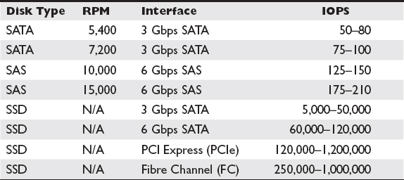
Table 1-1 Standard IOPS Ratings for SATA, SAS, and SSD Disks
Capacity vs. Speed
Determining the right storage for the job starts with determining the requirements of capacity and speed. Capacity involves how much space the system or application requires, and speed is how fast the storage needs to be. I/O and throughput were discussed in the previous section, providing an understanding of how to measure the speed of a device. An application may also have a speed requirement, which is often represented in IOPS. Disks may need to be combined to obtain the necessary capacity and speed for the application. For example, an application requires 5,000 IOPS and 2TB capacity; 600GB 15,000 rpm SAS disks that get 175 IOPS and 200GB SSD disks that get 4,000 IOPS are available for use. Twenty-nine SAS disks would be necessary to get 5,000 IOPS, and this would provide more than enough capacity (17.4TB). Alternatively, two SSD disks would provide the necessary IOPS but not the required capacity. It would take ten SSD disks to reach the required 2TB capacity, which would be more than enough IOPS at this point. These rough calculations assume that all disks would be able to be used concurrently to store and retrieve data, which would offer the most ideal performance circumstances. The “RAID Levels” section will show different methods for combining multiple disks and how they can be used to gain additional speed and prevent against data loss when one or more disks fail.
Available Disk Interfaces and Their Characteristics
Interfaces are the connection between data storage devices and other devices such as computers, networks, or enterprise storage equipment. Internal interfaces connect storage devices within a computer or storage system, while external interfaces connect to stand-alone storage equipment such as disk enclosures, tape libraries, or compact disc jukeboxes.
A variety of interfaces have been introduced over the years, some designed for high cost and high performance with a large amount of throughput and others designed for lower cost and lower performance.
ATA
Versions of Advanced Technology Attachment (ATA) provide a low-cost, low-performance option and are ideal when a large amount of storage is needed but does not have to be accessed directly by end users or applications. Examples of good uses of ATA include backup storage or storage for infrequently used data.
PATA
Parallel ATA (PATA), also known as Integrated Drive Electronics (IDE), was introduced in 1986 and standardized in 1988. It was the dominant interface used for HDDs and CD-ROM drives until 2003. PATA disks were originally referred to only as ATA disks, but the acronym PATA now differentiates these disks from SATA disks. The IDE name is derived from the fact that PATA disks have a controller integrated onto the disks instead of requiring a separate controller on the motherboard or expansion card. The integrated controller handles commands such as moving the actuator arm, spinning the disk up, and parking the heads.
A PATA cable, depicted in Figure 1-3, has 40 or 80 wires that make contact with the connectors on the disk and the motherboard. PATA cables also have a maximum length of 18 inches. Data is transferred in parallel, meaning that multiple bits of data are transferred at once. The number of bits transferred in a single operation is called the data bus width; in the case of PATA, it is 16.
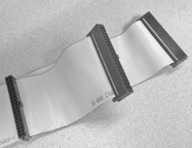
Figure 1-3 A PATA cable
Up to two devices may be attached, but in order for both to share the same cable, one device must be configured as the master (device 0) and the other as the slave (device 1). The master or slave setting is configured by a jumper on the back of the PATA device, depicted in Figure 1-4. Some devices support a mode called cable select, whereby the device automatically configures itself as master or slave depending on its location on the cable.
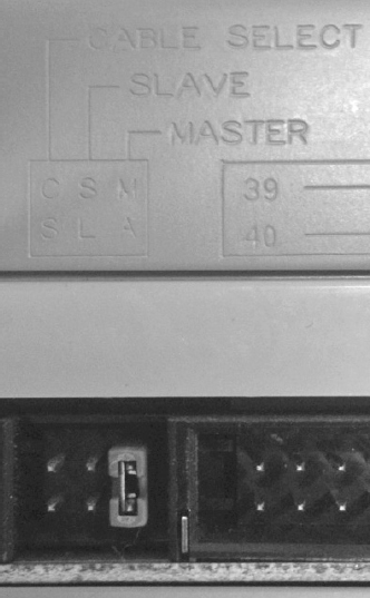
Figure 1-4 A jumper for the master, slave, or cable select setting
PATA cables are a shared medium allowing only one device to communicate over the cable at a time. Connecting multiple devices to a single connector can impact the performance of the devices if disk operations execute on both disks at once, as is common when transferring files between disks or when installing software from a CD-ROM attached to the same cable. While earlier computers typically were equipped with two connectors on the motherboard, supporting up to four PATA devices, most computers today do not even include a PATA port on the motherboard. The best practice in this case is to place highly used devices on separate cables and pair lesser used devices with highly used ones so as to give each device maximum time on the cable.
PATA disks are powered by a plug with four pins and four wires known as a molex connector. The molex connector has one yellow 12-volt wire, one 5-volt red wire, and two black ground wires.
The last version of PATA, called Ultra ATA/133, had a maximum theoretical transfer rate of 133 MBps that was quickly eclipsed by SATA. Table 1-2 lists the PATA versions and their significant properties. Note that megabytes per second (MBps) is different from megabits per second (Mbps). There are eight bits in a byte, so the megabit transfer speed is eight times the megabyte transfer speed.
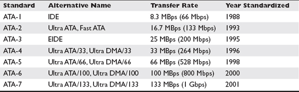
Table 1-2 PATA Versions
SATA
Serial ATA (SATA) was introduced in 2003 to replace the aging PATA. The parallel architecture of PATA created difficulties for exceeding the 133-MBps limit because its parallel transmissions were susceptible to electromagnetic interference (EMI) among the wires in the bus. SATA, however, runs on lower voltages and uses a serial bus, so data is sent one bit at a time. These enhancements bypassed some of the problems faced with PATA and allowed for higher transfer rates. SATA utilized the ATA command set, making it easier for equipment to include SATA ports since ATA was already supported on a wide variety of systems and BIOSs. SATA disks can also be connected as an external disk using an eSATA cable and enclosure, which offers faster speeds than external disks connected over USB or IEEE 1394 FireWire. Table 1-3 provides the speeds of each of these external disk technologies.
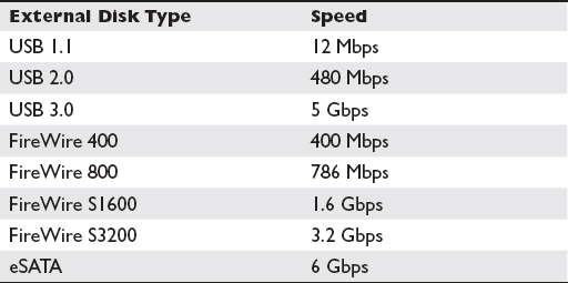
Table 1-3 External Disk Speeds by Type
SATA cables have seven connectors and a maximum length of 39 inches. SATA disks do not use a molex connector. Instead, the SATA power connector is smaller with 15 pins. Only one device can be connected to a cable, meaning the issue of a shared bus with master and slave designations does not exist with SATA disks. There have been multiple generations of SATA, depicted in Table 1-4. It should be noted that the bit per second transfer rates are not what one would expect since they are ten times the megabyte rate. This is intentional because SATA uses 8b/10b encoding. This form of encoding uses ten bits to represent one byte. The extra two bits are used to keep the clock rate the same on the sending and receiving ends.
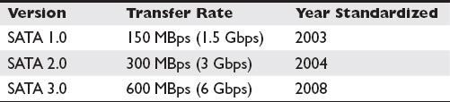
Table 1-4 SATA Versions
What really differentiates SATA from previous interfaces is the host of new features added along the way. Some of the features include
• Command queuing Command queuing optimizes the order in which operations are executed in a disk, based on the location of data. Without command queuing, operations are processed in the order they are received. Command queuing reorders the operations so that the data can be fetched with minimal actuator and platter movement.
• Hot-pluggable/hot-swappable This option allows a disk to be plugged or unplugged from a system while the system is running. Systems without hot-plug interfaces will need to be restarted before disks can be added or removed.
• Hard disk passwords SATA devices supporting this feature allow disks to be password protected by setting a user and a master password in the BIOS. User passwords are designed to be given to the primary user of a machine, while the master password can be retained by IT administrators. In this way, should an individual leave or forget their password, IT administrators can still unlock the disk. Once the disk is password-protected, each time the machine is started up, a prompt appears requiring the password to be entered. This password will be required even if the hard disk is moved to another machine. Hard disk passwords can also be synchronized with BIOS system passwords for ease of administration.
• Host protected area (HPA) HPA reserves space on the hard disk so that the system can be reset to factory defaults, including the original operating system, applications, and configuration that shipped with the machine. HPA space is hidden from the operating system and most partitioning tools so that it is not accidentally overwritten.
SCSI
Small Computer System Interface (SCSI) was standardized in 1986 and was the predominant format for high-performance disks for almost 30 years. There have been many versions of SCSI along with different cable types and speeds, as shown in Table 1-5. Internal SCSI uses ribbon cables similar to PATA. Over the years, 50-, 68-, and 80-pin connectors have been used. The last few versions of SCSI to be used shared much in common; and despite so many variations, expect to find the SCSI that uses a 16-bit bus supporting 16 devices and the connection types of 68 and 80 pin. SCSI’s max speed is 640 MBps, or 5,120 Mbps. You will typically find 68-pin cables connecting SCSI devices within a server, such as the connection between a SCSI controller card and the disk backplane; but the connection between disks and the backplane most often uses the hot-pluggable 80-pin connector known as Single Connector Attachment (SCA).
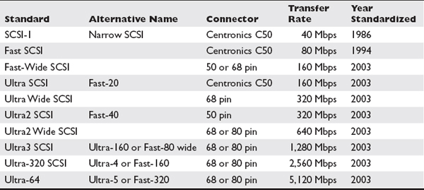
Table 1-5 SCSI Versions
Devices on a SCSI bus are given an ID number unique to them on the bus. This was originally performed using jumpers on the back of SCSI devices similar to the master slave configuration on PATA, but more recent disks allow for the SCSI ID to be configured automatically by software or the SCSI adapter BIOS. Up to 16 devices can exist on a single bus.
Each device on a SCSI bus can have multiple addressable storage units, and these units are called logical units (LUs). Each LU has a logical unit number (LUN). You will not find a new machine today equipped with SCSI, but the command set and architecture are present in many current technologies, including SAS, Fibre Channel, and iSCSI.
Fibre Channel
Fibre Channel (FC) picks up in enterprise storage where SCSI left off. It is a serial disk interface with transfer speeds of 2, 4, or 8 Gbps. The latest versions of FC disks use a 40-pin Enhanced SCA-2 connector that is SFF-8454 compliant, and they are hot-pluggable, so they can be added or removed while the system is powered on without interrupting operations. They utilize the SCSI command set and are commonly found in enterprise storage arrays. FC disks are expensive compared to other disk types.
SAS
Serial Attached SCSI (SAS) is a high-speed interface used in a broad range of storage systems. SAS interfaces are less expensive than FC, and they offer transfer speeds up to 1.2 GBps (12 Gbps). The SAS interface uses the same 8b/10b encoding that SATA uses. Thus, converting from bits per second to bytes per second requires dividing by ten instead of eight. SAS can take advantage of redundant paths to the storage to increase speed and fault tolerance. SAS expanders are used to connect up to 65,535 devices to a single channel. SAS cables can be a maximum of 33 feet long. The SAS connector is similar to the SATA connector except that it has a plastic bridge between the power and interface cables. This allows for SATA disks to be connected to a SAS port, but SAS disks cannot be connected to a SATA port because there is no place for the bridge piece to fit.
SAS version 1 (SAS1) was limited to transfer speeds of 300 Mbps (3 Gbps), but SAS version 2 (SAS2) achieves transfer speeds of 600 Mbps (6 Gbps), with the latest SAS3 disks released in late 2013 reaching speeds of 1.2 GBps (12 Gbps). SAS2 and SAS3 are backward compatible with SAS1, so SAS1 and SAS2 drives can coexist on a SAS2 or SAS3 controller or in a SAS2 or SAS3 storage array, and SAS2 drives can likewise coexist with SAS3 drives on SAS3 arrays or controllers. However, it is not wise to mix SAS1, SAS2, and SAS3 drives in the same RAID array because the slower drives will reduce the performance of the array.
Multiple Disks for Larger Storage and Fault Tolerance
Storage professionals are often called on to create groups of disks for data storage. Grouping disks together allows for the creation of a larger logical drive, and disks in the group can be used to protect against the failure of one or more disks. Most groupings are performed by creating a Redundant Array of Independent Disks (RAID). To create a RAID, multiple disks must be connected to a compatible RAID controller, and controllers may support one or more types of RAID known as RAID levels. There are two designations for capacity. Raw capacity is the total capacity of disks when not configured in a RAID. For example, five 100GB disks would have a raw capacity of 500GB. Usable capacity is the amount of storage available once the RAID has been configured.
RAID Levels
Several RAID specifications have been made. These levels define how multiple disks can be used together to provide increased storage space, increased reliability, increased speed, or some combination of the three. Although not covered here, RAID levels 2 to 4 were specified but never adopted in the industry, so you will not see them in the field. When a RAID is created, the collection of disks is referred to as a group. It is always best to use identical disks when creating a RAID group. However, if different disks are used, the capacity and speed will be limited by the smallest and slowest disk in the group. RAID 0, 1, 5, and 6 are basic RAID groups introduced in the following sections. RAID 10 and 0+1 are nested RAID groups because they are made up of multiple basic RAID groups. Nested RAID groups require more disks than basic RAID groups and are more commonly seen in networked or direct attached storage groups that contain many disks.
RAID 0
RAID 0 writes a portion of data to all disks in the group in a process known as striping. At least two identical disks are required to create a RAID 0 group, and these disks make up the stripe set. Figure 1-5 shows how a file would be written to a RAID 0 consisting of four disks. The file is broken into pieces and then written to multiple disks at the same time. This increases both read and write speeds because the work of reading or writing a file is evenly distributed among the disks in the group. RAID 0 usable capacity is the total capacity of all disks in the stripe set and thus the same as the raw capacity. The main drawback to RAID 0 is its lack of redundancy. If one disk fails, all the data in the group is lost.
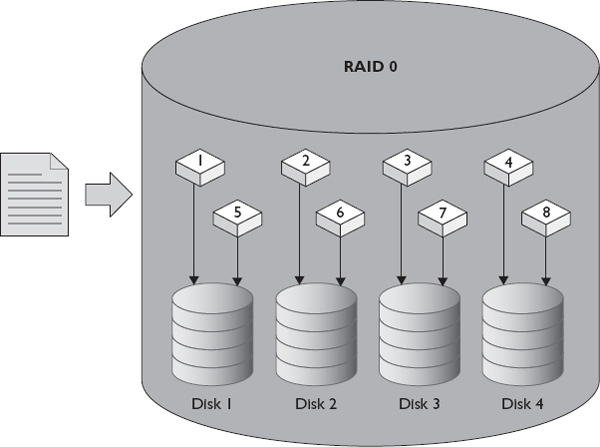
Figure 1-5 Writing a file to RAID 0
RAID 1
RAID 1 writes the data being saved to two disks at the same time. If a single disk fails, no data is lost, since all the data is contained on the other disk or disks. RAID 1 is also known as mirroring. Figure 1-6 depicts how a file would be stored on a two-disk RAID 1. The usable capacity of the mirror is the same as the capacity for one disk in the group, but because data can be retrieved from both disks simultaneously, mirroring results in a slight boost to read performance. When a failed disk is replaced in a RAID 1 group, the mirror is rebuilt by copying data from the existing disk to the new disk. This rebuild time has significant impact on group performance, even though it takes significantly less time to perform a rebuild on a RAID 1 than on a RAID 5. RAID 1 is good for high read situations since it can read data at twice the speed of single disks. However, it is not best for high write situations because each write must take place on both disks requiring the same time as a single disk.
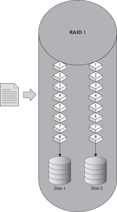
Figure 1-6 Writing a file to RAID 1
RAID 5
RAID 5 stripes data across the disks in the group, and because it also computes parity data and spreads this across the disks, if one disk in the group is lost, the other disks can use their parity data to rebuild the data on a new disk. RAID 5 requires at least three disks and, because of its speed, is popular. Figure 1-7 shows a file write to a RAID 5 array of four disks. Since parity data needs to be computed each time data is written, it suffers from a write penalty. Additionally, the parity data also takes up space on the group. The amount of space required diminishes as the number of disks in the group increases, but it takes more time to compute parity for larger RAID 5 groups. The equivalent of one disk in the group is used for parity, which means the usable capacity of a RAID 5 group can be computed by subtracting one from the number of disks in the group and multiplying that by the capacity of a single disk. For example, if six 1TB disks are placed into a RAID 5 group, the total capacity will be 5,000GB (5TB). We thus describe a RAID 5 group by listing the number of disks upon which the capacity is based and then the number of parity disks. Accordingly, making a six-disk RAID 5 group would be described as a 5+1.
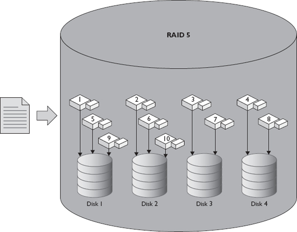
Figure 1-7 Writing a file to RAID 5
A RAID 5 group goes into a degraded state if a disk within the group is lost. Once that disk is replaced, the group begins rebuilding the data to the replaced disk. Group performance is significantly impacted while the group rebuilds, and a loss of any disks in the group, prior to completion of the rebuild, will result in a complete loss of data. Additionally, the increased load on the remaining disks in the group makes these disks more susceptible to a disk failure. Rebuild time increases with an increase in the capacity or number of disks in the group. Thus, a four-disk group takes longer to rebuild than a three-disk group, and a group of 3TB disks takes longer to rebuild than one made up of 1TB disks.
RAID 5 has good performance in high read situations because of its use of striping, and it has decent performance in high read situations but not as good as RAID 10 or RAID 1 because of the need for parity computations.
RAID 6
Although RAID 6 is similar to RAID 5, it computes even more parity data, and up to two disks can fail in the group before data is lost. RAID 6 requires at least four disks and suffers from an even greater write penalty than RAID 5. Consequently, the additional parity data of RAID 6 consumes the equivalent of two disks in the RAID group. Therefore, the usable capacity of the RAID group is the total disks in the group minus two. Figure 1-8 shows a file write to a RAID 6 array consisting of four disks. Similar to RAID 5 groups, RAID 6 groups can be described using the data and parity disks. This way, if a RAID 6 group is created from eight disks, it would be described as 6+2. A RAID 6 set made up of eight 500GB disks would have a usable capacity of 3,000GB (3TB). In spite of RAID 6 suffering from an even greater rebuild time, the group is not at risk for a total loss of data if another disk fails during the rebuild period.
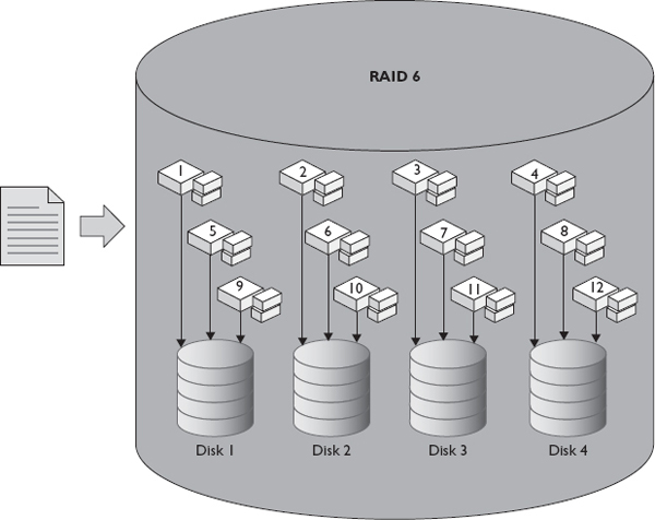
Figure 1-8 Writing a file to RAID 6
RAID 10 (1+0)
RAID 10 is a stripe made up of many mirrors. RAID 10 requires an even number of at least four disks to operate. Pairs of disks in the group are mirrored, and those mirrored sets are striped. RAID 10 offers the closest performance to RAID 0 and offers extremely high reliability as well since a disk from each of the mirrored pairs could fail before loss of data occurs. Figure 1-9 shows how a file would be written to a RAID 10 array of eight disks. The main drawback of RAID 10 is its total capacity. Since RAID 10 consists of many mirror sets, the usable capacity is half the raw capacity. A ten-disk RAID 10 group made up of 100GB disks would have a usable capacity of 500GB and a raw capacity of 1TB (1000GB). This disk configuration would be described as 5+5. RAID 10 rebuild times are comparable to those of RAID 1, and the performance impact of a failed disk will be much shorter in duration than had it occurred on a RAID 5 or RAID 50. RAID 10 is best for high read situations since it can read from the stripes and mirrors of all the disks in the RAID set. It is good for high write situations since it uses striping and there is no parity computation.
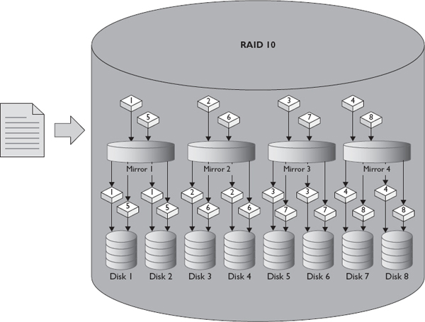
Figure 1-9 Writing a file to RAID 10
RAID 0+1
RAID 0+1 is a mirror of stripes—the opposite of RAID 10. RAID 0+1 does not have the same reliability as RAID 10 because a loss of a disk from both mirrors would result in a total loss of data. RAID 0+1 can, however, sustain a multiple-disk failure if the failures occur within one of the stripe sets. RAID 0+1 is less commonly implemented because most implementations favor RAID 10. RAID 0+1 has fast rebuild times similar to RAID 10. Figure 1-10 shows how a file would be written to a RAID 0+1 array of eight disks.
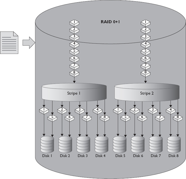
Figure 1-10 Writing a file to RAID 0+1
RAID 50
RAID 50 is a stripe made up of multiple RAID 5 groups. A RAID 50 can be created from at least six drives. RAID 50 offers better performance and reliability than a single RAID 5 but not as much as a RAID 10. However, RAID 50 offers greater capacity than a RAID 10, so it is often used when performance requirements fall in between RAID 5 and RAID 10. One drive from each RAID 5 group in the RAID 50 can fail before loss of data occurs. The usable capacity for a RAID 50 depends on how many RAID 5 sets are used in the construction of the RAID 50.
Similar to a RAID 5, rebuild times increase with an increase in the capacity or number of drives in the group. However, the rebuild time for a loss of a single drive in a RAID 50 group would be much faster than a single drive loss in a RAID 5 group with a similar number of disks because the rebuild effort would be isolated to one RAID 5 within the RAID 50. Performance would still be degraded because the degraded RAID 5 is within the overall stripe set for the RAID 50 group, so each new data operation would need to access the degraded RAID 5.
RAID 51
RAID 51 is a mirror of RAID 5 groups. This provides more reliability than RAID 5 and RAID 50, and the usable capacity of the set is half the total number of drives minus one; therefore, if there were ten 100GB drives in a RAID 51, the total capacity would be 400GB because five drives are used in the second RAID 5 set that is mirrored and one drive is used in each of the RAID 5 sets for parity. The parity drive in the mirrored set is already accounted for, so you subtract out the parity drive from the first set to get the usable capacity. RAID 51 can sustain a loss of multiple drives up to an entire RAID set as long as not more than one drive has failed on the other mirrored RAID 5 set.
RAID 51 rebuild times can be quite short because the data from the identical unit in the mirrored RAID 5 can be used to build the faulty drive. However, some implementations of RAID 51 use multiple controllers to protect against RAID controller failure. If this is the case, RAID 51 rebuild times will be comparable to RAID 5 because rebuilds take place within the controller, so the data from the mirror set cannot be used to rebuild individual drives on another controller.
RAID 51 is often used with two RAID controllers. Both controllers host a RAID 5 array, and the arrays are mirrored. If an entire controller fails, the RAID 51 is still accessible because it can operate in failover mode on the other RAID 5 set and controller until the controller and/or drives are replaced in the other RAID 5 set.
JBOD
Just a Bunch of Disks (JBOD) is not a RAID set, but it is a way to group drives to achieve greater capacity. JBOD uses a concatenation method to group disks, and data is written to a disk until it is full; then data is written to the next disk in the group. JBOD does not offer higher availability because the loss of a single drive in the group will result in a loss of all data. JBOD, however, is simple to implement, and it results in a usable capacity that is the same as its raw capacity. Use JBOD when you need the maximum usable capacity and when the reliability of the data is not a concern.
Hosts Interaction with Disks
To be used, storage must be made available to hosts. Hosts store and organize data in a directory structure known as a file system, and file systems exist on logical volumes that can be made up of one or more physical volumes.
A physical volume is a hard disk; a portion of a hard disk, called a partition; or, if the storage is remote, a LUN. One or more physical volumes can be combined on the host into a volume group. The volume group can then be divided into manageable sections known as logical volumes. Thus, a physical disk may have multiple logical volumes, and a logical volume may have multiple physical disks. Figure 1-11 depicts the relationship between these concepts.
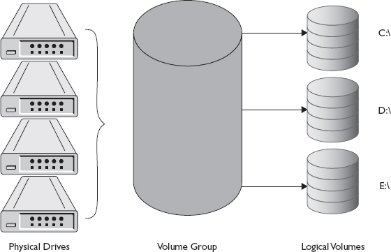
Figure 1-11 Physical disks, volume groups, and logical volumes
For a system to use a logical volume, it must be mounted and formatted. Mounting the volume establishes the location where it can be referenced by the system. In Unix and Linux, this location is often a directory path. In Windows, mount points are usually given a drive letter, which is referenced with a colon and a forward slash such as C:. Windows also allows drives to be given directory mount points similar to Linux and Unix systems.
The formatting process establishes a file system on the logical volume and sets a cluster size. The cluster size is how large of chunks the file system will divide the available disk space into. Larger cluster sizes result in fewer chunks of larger size, and this makes it faster for the system to read large data files into memory. However, if many small files are stored on the system with large cluster sizes, clusters will be padded to fill up the remaining space in the cluster, which will decrease available space and performance. Understand the size of files that will be stored on a system before configuring the cluster size. Additionally, the stripe size on RAID 0, RAID 5, and RAID 6 volumes is often a configurable option on the RAID controller. The stripe size is the size of each chunk that is placed on the disks when files are split into pieces. Select a stripe size that is a multiple of the cluster size you will use when formatting the logical drive. You can take the number of disks in the stripe and divide by the cluster size to find an optimal number. Stripe and cluster size selections are powers of 2, so a four-disk stripe for a 512KB cluster might use 64KB or 128KB stripes since these numbers divide evenly into 512. This will ensure that file reads and writes will be distributed evenly across the stripe set.
File Systems
File systems are used to organize data on a logical drive. File systems track the location of files on the disk and file metadata. Metadata is data about the file such as creation date, last modified date, author, and permissions. File systems are structured hierarchically, beginning with a root directory under which other directories can be created. File systems also collect information used to track faulty areas of the drive.
Some file systems are journaled. Journaled file systems write file metadata to a journal before creating or modifying a file on the file system. Once the file has been created or modified, metadata is also modified. The journal protects against corruption should the drive or system go offline while the file operation is in progress. The journal can be used to determine whether files on the file system are in an inconsistent state, and sometimes the files can be corrected by using the journal data. Journaling increases the amount of time required to write files to the file system, but many file systems today use it to protect data integrity.
A file system is created by formatting a logical drive. Formatting consumes some of the available space on the drive, resulting in a lower-capacity value for a formatted disk than an unformatted one. However, it is an essential step in order to use the available space on the drive. A file system type can depend on the operating system being used when beginning the formatting process.
Whereas a controller identifies data based on CHS, logical volumes map blocks using logical block addressing (LBA). LBA is a way of referencing a location on a disk without a device having knowledge of the physical disk geometry. LBA provides a system with the number of blocks contained on the drive while the system keeps track of the data contained on each block. It requests the data by block number, and the drive then maps the block to a CHS and retrieves the data. Blocks are numbered starting with cylinder 0, head 0, and sector 1 and continuing until all sectors on that cylinder and head are read. The numbering starts again with head 1, which would be the bottom of the first platter, and continues along cylinder 0. This progresses until sectors for all heads in cylinder 0 are counted, at which time the process begins again for cylinder 1. The block count continues until all sectors for all heads and cylinders are accounted for.
Chapter Summary
A hard disk drive is a component of storage systems, computers, and servers that is used to store data. HDDs consist of round flat surfaces known as platters that rotate on a spindle. The platters are organized into cylinders and sectors. Disk heads write data to the platters by aligning a substrate on the platters using an electromagnetic field. Solid-state drives store data by retaining an electrical current in a gate. Control gates allow current to be placed into floating gates. These floating gates can hold one or more binary numbers depending on the type of solid-state cell in use. MLC disks can hold more than one binary number per cell to achieve a greater capacity than SLC disks, which hold only one binary number per cell. However, MLC disks do not last as long as SLC disks, and they have lower performance.
Interfaces are used to connect disks to other components in a computer or storage system. The ATA interfaces PATA and SATA offer a low-cost interface for lower performance needs, while SCSI, FC, and SAS disks are used for high-performance storage.
A single disk often does not provide enough speed and resiliency for business applications, so disks are grouped together into a RAID set. RAID 0 writes pieces of data to multiple disks to improve speed in a process known as striping. Read and write operations are divided among the disks in the set, but a loss of a single disk causes a loss of data on all disks in the stripe set. RAID 1 stores identical data on two disks in a process called mirroring. RAID 5 uses striping to achieve high-data speeds while using parity data to protect against the loss of a single disk in the set. RAID 6 operates similarly to RAID 5, but it calculates additional parity to protect against the loss of two disks in the set. RAID 10 and RAID 0+1 combine striping and mirroring to achieve higher performance and resiliency than RAID 5 or 6. RAID 10 and RAID 0+1 can lose up to half the disks in a set before data is lost.
Hosts interface with storage by using logical volumes. A logical volume can be a portion of a single disk, or it can be multiple physical disks together. The host uses a file system to organize the data on the logical volume. Hosts format a logical volume to create the initial file system and make the volume ready for use. The logical volume is then mounted into a directory or as a drive letter.
Chapter Review Questions
1. Which of the following components would not be found in a solid-state drive?
A. Controller board
B. Cache
C. Spindle
D. Interface
2. You are configuring a server that will store large database backups once a day. Which interface would give you the greatest capacity at the lowest price?
A. SAS
B. FC
C. SATA
D. SCSI
3. A head does which of the following?
A. Controls the flow of data to and from a hard drive
B. Aligns tiny pieces of metal using an electromagnetic field
C. Serves as the starting point in a file system under which files are created
D. Connects platters in a hard drive and spins them at a consistent rate
4. Which of the following statements is true about RAID types?
A. RAID 1 is known as striping, and it writes the same data to all disks.
B. RAID 0 is known as mirroring, and it writes pieces of data across all disks in the set.
C. RAID 5 uses mirroring and parity to achieve high performance and resiliency.
D. RAID 1 is known as mirroring, and it writes the same data to all disks.
5. You have created a RAID set from disks on a server, and you would like to make the disks available for use. Which order of steps would you perform?
A. Create a logical volume, mount the logical volume, and format the logical volume.
B. Format the logical volume, mount the logical volume, and create a directory structure.
C. Create a directory structure, mount the logical volume, and format the logical volume.
D. Create a logical volume from the RAID set, format the logical volume, and mount the logical volume.
6. Which interface can transmit at 6 Gbps?
A. SATA and SAS
B. Fibre Channel
C. SCSI
D. PATA
7. Which of the following is an advantage of IOPS versus other metrics such as seek time or rotational latency?
A. IOPS identifies whether an individual component in a system is exhibiting acceptable performance.
B. IOPS measures end-to-end transfer to provide a single metric for transmission.
C. The IOPS metric is specified by the IEEE 802.24, so it is implemented consistently across all hardware and software that is IEEE 802.24 compliant.
D. IOPS eliminates the need to run further benchmarking or performance tests on equipment.
8. A customer needs 250GB of storage for a high-performance database server requiring 2,000 IOPS. They want to minimize the number of disks but still provide for redundancy if one disk fails. Which solution would best meet the customer’s requirements?
A. RAID 1 with two 3,000 IOPS 128GB solid-state drives
B. RAID 5 with three 3,000 IOPS 128GB solid-state drives
C. RAID 5 with seven 350 IOPS 300GB SAS drives
D. RAID 0 with two 3,000 IOPS 128GB solid-state drives
Chapter Review Answers
1. C is correct. The spindle would not be found in an SSD because SSDs do not have moving parts.
A, B, and D are incorrect because SSDs consist of flash memory cells, a controller board, a cache, and an interface.
2. C is correct. Performance was not a concern in this question. The only requirement was for capacity and lowest cost, so SATA disks would be the best fit.
A, B, and D are incorrect because SATA disks are less expensive per gigabyte than SAS, FC, or SCSI. Additionally, SATA disks come in larger capacities than SCSI disks.
3. B is correct. The head is a small electromagnet that moves back and forth on an actuator arm across a platter. The head generates an electromagnetic field that aligns the substrate on the platter in the direction of the field. The field direction is determined based on the flow of current in the head. Current can flow in one of two directions in the head.
A, C, and D are incorrect. Data flow is controlled by the drive controller, so A is incorrect. C is incorrect because the starting point in a file system is the root. D is incorrect because the spindle connects platters in a hard drive and spins them at a consistent rate.
4. D is correct. RAID 1 is mirroring. The mirroring process writes identical data to both disks in the mirror set.
A, B, and C are incorrect. A is incorrect because RAID 1 is not known as striping. RAID 0 is known as striping. B is incorrect because it is not known as striping. The rest of the statement is true about RAID 0. C is incorrect because RAID 5 uses striping and parity, not mirroring and parity. Mirroring is used in any of the RAID implementations that have a 1 in them, such as RAID 1, RAID 10, and RAID 0+1.
5. D is correct. A logical volume must be created from the RAID set before the volume can be formatted. Mounting occurs last. The step of creating a directory structure is not required for the disk to be made available.
A, B, and C are incorrect because they are either not in the right order or they do not contain the correct steps. It is not necessary to create a directory structure, as this is performed during the format process.
6. A is correct. SATA version 3 and SAS both support 6-Gbps speeds.
B, C, and D are incorrect. Fibre Channel supports speeds of 2, 4, or 8 Gbps. SCSI has a max speed of 5,120 Mbps, while PATA has a max speed of 133 Mbps.
7. B is correct. IOPS measures the transfer rate from the point at which the IOPS metric is initiated to the storage device.
A, C, and D are incorrect. A is incorrect because IOPS does not identify an individual component. C is incorrect because the IOPS metric is not standardized by the IEEE. The 802.24 deals with smart grids and has nothing to do with IOPS. D is incorrect because other metrics may be needed to diagnose where performance issues lie or to document granular metrics on individual components.
8. A is correct. Two SSD disks would achieve the required IOPS and still provide for redundancy if one disk fails.
B, C, and D are incorrect. Options B and C use more disks than option A, so they are not ideal, and option D does not provide redundancy in the case of disk failure.
..................Content has been hidden....................
You can't read the all page of ebook, please click here login for view all page.