Chapter 6

Syntax-Directed Translation

Syntax-directed definition is a generalization of a context free grammar (CFG), but effectively is an attribute grammar. Syntax-directed translation describes the translation of language constructs guided by CFGs. They are used in automatic tools like YACC.

Syntax-directed translation is an extension of context free grammars (CFGs). This helps the compiler designer to translate the language constructs directly by attaching semantic actions or subroutines. In this chapter, we discuss what is syntax-directed translation (SDT), how to write SDT”s, and how to evaluate semantic actions. We also discuss the different types of SDT”s and how to write S-attributed definition and L-attributed definition in detail. Converting L-attributed to simple attributed is also discussed.

6.1  Introduction

So far we have discussed parsing. Given a grammar, how a parser checks the syntax of programming language construct. Now let us look at another technique called syntax-directed translation with which we can combine many tasks along with parsing. Along with each production of the grammar, we attach a semantic action. The grammar together with semantic action is called syntax-directed translation (SDT).

      A → α + {action} = SDT

Semantic action or translation rule or semantic rule or action is the same. We can attach semantic actions for grammar rules for performing different tasks. Examples are:

1. To store/retrieve type information in symbol table
2. To perform consistency checks like type checking, parameter checking, etc.
3. To issue error messages
4. To build syntax trees
5. To generate intermediate or target code

There are two ways of defining semantic rules. One is syntax-directed definition (SDD), which is a high-level language specification for translation. This hides many implementation details and frees the user to explicitly specify the order of evaluation. The other scheme syntax-directed translation (SDT) specifies the order in which semantic rules are to be evaluated. So they allow some implementation details to be shown. Here we use the names SDD or SDT interchangeably but the basic difference between the two is in specifying the evaluation order. With SDD/SDT, we parse the input, create parse tree, and traverse the parse tree as needed to evaluate semantic actions at the parse tree nodes. Evaluation of semantic rules may result in storing information in symbol table, issue error diagnostics or other activities.

Here we discuss syntax-directed translations. They are also called attribute grammars, where

• Each grammar symbol is assigned certain attributes.
• Each production is augmented with semantic rules which are used to define attribute values

6.2  Attributes for Grammar Symbols

Syntax-directed translation is a generalization of a context free grammar in which each grammar symbol has an associated set of attributes. If we consider parse tree node as a record for holding information, then an attribute is the name of each field in record. A grammar symbol can have “n” attributes. The attributes for grammar symbol can be a type, value, address, pointer, or a string. The attributes that can be associated with a grammar symbol can be classified into two types as defined below.

Attribute types:

1. Synthesized attribute—The value of a synthesized attribute at a node is computed from the values of attributes at the children of that node in the parse tree.

   EX: A → XYZ

   Here in Figure 6.1 we assume that there is an attribute .”s” with each grammar symbol. Then if it is evaluated as A • s = f(X • s | Y • s | Z • s) that is,

   A → XYZ       {A • s = X • s + Y • s + Z • s}

   Then .”s” is called the synthesized attribute.

2. Inherited attribute—The value of an inherited attribute is computed from the values of attributes at the siblings and parent of that node.

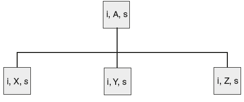
Figure 6.1 Parse Tree for Rule A → XYZ

In Figure 6.1, we assume that there is an attribute “i” with each grammar symbol. Then if it is evaluated as Y • i = f (X • i | Z • i | A • i | A • s) that is, 

  A → XYZ {Y • i = A • i + X • i + Z • i}

  Then “•i” is called the inherited attribute. 

Once we consider an attribute as a synthesized attribute, wherever it is used, it should preserve the basic property of the synthesized attribute, that is, the value at parent is evaluated with attribute values of its children. We cannot use the same attribute as synthesized for some time and inherited for some time. Generally, we don’t specify explicitly, whether an attribute is synthesized or inherited, by looking at semantic actions, that is, dependency of attribute, we need to understand whether it is synthesized or inherited.

6.3  Writing Syntax-Directed Translation

Let us see how to write SDT. Let us try to understand with an example. Consider parsing the input string “1 + 2 * 3.” Recollect, how a bottom-up parser parses this string. It uses the following grammar:

 

      E → E + T | T

      T → T * F | F

      F → num

 

Parses the string. The result is a parse tree as shown in Figure 6.2.

Now along with parsing, that is, checking the syntax of a string, if we want to perform the evaluation of an expression, let us see how to write SDT. So here the additional task that is combined with parsing is evaluation of expression. For this we need to attach semantic rules. Parse tree gives us the order in which reductions are carried out by the parser. If we follow the tree from bottom to top we get the order. For example in Figure 6.2, the order of reductions is number to F, F to T, T to E, next number to F, F to T, then number to F, T * F to T, E + T to E. This is very useful to think about semantic actions. Whenever parser reduces by rule, we must think what should be the corresponding action to get the desired output. In SDT, initially we assume that whenever a bottom-up parser reduces by production, the corresponding action is automatically carried out.

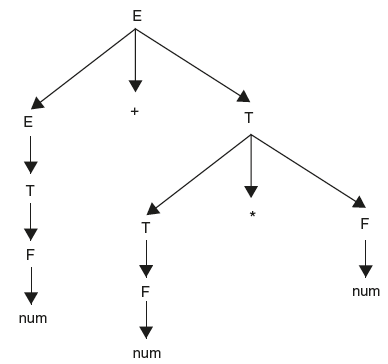
Figure 6.2 Parse Tree for Expression Grammar

How do we define semantic rules? Here first we need to find out what additional information is required. When a bottom-up parser sees the input string “1 + 2 * 3,” on reading the first symbol “1,” it gets a token from the lexical analyzer as “num.” Now the first step performed by the parser is token “num” reduced to F by using production F → num. If it is only checking the syntax, this reduction is enough. But along with this, if we want to take care of the evaluation of expression, reducing first token to nonterminal alone may not be sufficient. To take care of the evaluation of expression at any time, we have to propagate additional information along with nodes of the parse tree. That additional information here is lexeme value of token “num.” So to store the additional information, first we need to assume an attribute with grammar symbol. We attach attribute to grammar symbol with”.” We assume that there is an attribute “.val” with each grammar symbol. Once attribute is present, it will be for all grammar symbols like E.val, T.val, F.val. Now semantic actions define how to evaluate this attribute values at any node in the parse tree.

For example, when the parser reduces “num” to F by using production F → num, we need to store the attribute value at node F. Hence, we attach semantic action as {F.val = num.lval;} where num.lval is lexeme value of token num. It can be any value at run time like “1” or “2” or “3” or “1000.” So the result is as shown in Figure 6.3.

The next step in parsing is reducing F to T. So here semantic action is forwarding lexeme value from F to T by attaching semantic action {T•val = F•val;}. The same thing happens with T to E also. The result in shown below in Figure 6.4.

Next the parser reads the next token “+,” and then “2.” Now it gets a token num and reduces that to F. As translation for T → F is already defined, value “2” is propagated to node F and then to node T also. Next the parser reads the next token “*,” then “3.” Now it gets a token num and reduces that to F. Now the parser reduces T * F; here the semantic action is to evaluate the expression and store the result. So SDT is defined as follows:

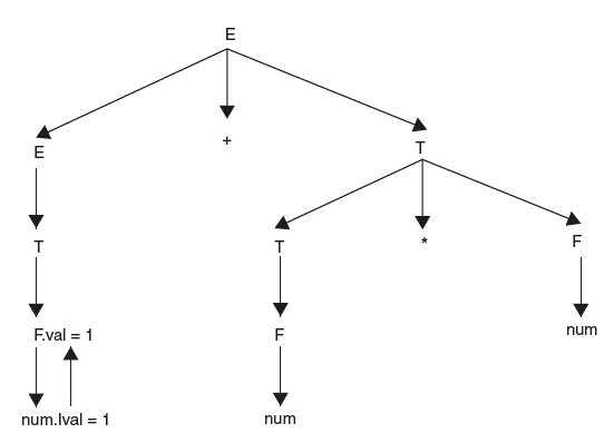
Figure 6.3 Parse Tree with Attribute Values

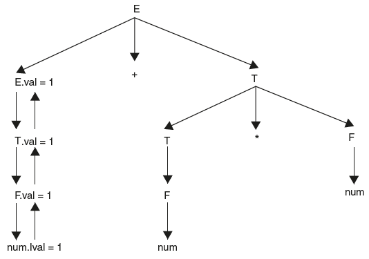
Figure 6.4 Parse Tree with Attribute Values

Example 1:

SDT for evaluation of expressions/Desk calculator

 

	E → E1 + T	{E•val = E1•val + T•val}
	E → T	{E•val = T•val}
	T → T1 * F	{T•val = T1•val * F•val}
	T → F	{T•val = F•val}
	F → id	{F•val = num•lval}

 

Here E or E₁ is the same. Just to understand the semantic action, this notation is used. Here num.lval is the lexeme value of token num. The result of carrying out actions is shown in Figure 6.5.

The parse tree that shows attribute values at each node is called annotated or decorated parse tree as shown in Figure 6.5.

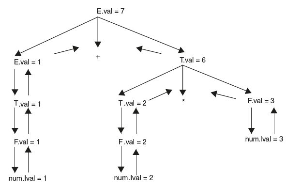
Figure 6.5 Annotated Parse Tree

New semantic actions can be added without disturbing the existing translations.

As we have seen in the first example, let us understand the procedure for writing SDTs. It involves the following three steps:

1. Define grammar for input string.
2. Take a simple string and draw a parse tree.
3.  Attach semantic actions by looking at the expected output.

Parser always starts with grammar. Here the second step is constructing the parse tree. Drawing the parse tree has two advantages. One is to check whether defined grammar is right or wrong, another is to get order in which reductions are carried out. This order is important to define semantic action. Follow the same order, and think about semantic action. Let us understand the procedure with one more example.

Example 2:

Write an SDT for converting infix expressions to post fix form, that is, given an input string “a + b * c” should give “abc * +” as output.

Let us see how to write the SDT. The first step is define the grammar. As input is the same as the previous example, the same grammar can be used. Semantic actions are not the same because the expected output is different. Now take a simple string “a + b” and draw a parse tree as shown Figure 6.6.

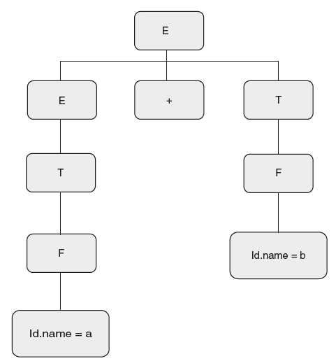
Figure 6.6 Parse Tree for String “a + b”

Look at Figure 6.6.

1. The parser first reads “a”; it will be matched with the token “id.” Now look at output, “ab +”; whatever is read should appear in output. So let the semantic action with reduce action F → id be {print(“id•name”);}, where “id.name” is the name of the identifier, whether it is “a” or “b “or “c.”
2. Now look at the next step performed by the bottom-up parser T → F. Here during this reduction, do we have to propagate any additional information? No. As there is no additional information to be propagated, there is no need of assuming attributes to grammar symbols. So with reduce action T → F, there is no need of any semantic action. Hence, we define the translation as T → F {}. Same thing happens with E → T also.
3. Next parser reads “+.” Just with E+, it cannot perform any reduce action; Hence reads “b.”

   Now “b” is reduced to F, here “b” is printed out as F→ id {print(“id•name”);}.

   Then it reduces, F to T, and there is no action.

4. The next reduction is “E + T” by E. Here already “ab” is printed and the only left out character to be printed is the operator “+.” So whenever an expression is reduced, print operator. Add this as semantic action with the rule. The resulting SDT is shown below

SDT for converting infix to postfix expression

 

Let us understand how to define semantic action by taking one more example. The next phase in parsing is semantic analysis. The semantic analyzer’s main function is type checking. Let us write a simple type checker.

Example 3:

Write an SDT for a simple type checker. Here we assume that our type checker is very simple and recognizes only three types—int, bool, and err. Here “int” type is for integers, “bool” type is for Boolean values True/false and “err” type is for error. Here we would like to have a type checker that checks for expressions of the form: (8 + 8) = = 8. Given such expression, it should check the type compatibility of operands and the final result is true/false, that is, bool.

1. Define grammar. Grammar is for expressions. Why do we have to consider unambiguous grammars? Let us take ambiguous grammar. We have already discussed how to construct parsers with ambiguous grammars also. So define grammar as follows.

    

   E → E+ E

   E → E and E

   E → E = = E

   E → true

   E → false

   E → num

   E → (E)

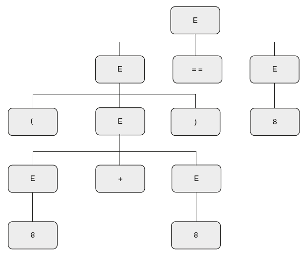
2. Take the input string and draw a parse tree for string “(8 + 8)==8” as in Figure 6.7.
3. Now let us attach semantic actions. First the parser reads “(“ and then “8.” Here we are not interested with value; what we are writing is a type checker. A type checker first should collect type information, and then should verify type compatibility of operands. Here when “8” is read, we need to collect and store type information. For storing type information, we assume that there is an attribute .”type” with each grammar symbol. So when token num is reduced to E after reading “8,” we define semantic rule as { E●type=int;} because “8” is integer type. Similarly for true/false, assign the type as bool.
4. Now the parser reads “+,” then “8,” and reduces “8” to E. Now the next reduction is E + E to E. Here type checker should verify types. To distinguish between left hand side nonterminal E and operands on right hand side Es,“we take them as E₁, E₂, and E₃ respectively. When expression with arithmetic addition is reduced, type check could be checking if both operands are integer type. If they are integers, it returns integers, or else it returns an error type. The above semantics can be implemented by attaching the semantic action as follows:
   

   Figure 6.7 Parse Tree for String “(8 + 8) = = 8”

   E₁ → E₂ + E₃ { if( E₂•type = =int and E₃•type = =int)

   then E₁•type = int else E_1•type=error;}

5. Similarly, if an expression with Boolean operator is reduced, type check could be checking if both operands are integer type or Boolean type. If they are int/bool, return bool, else return error type. The above semantics can be implemented by attaching the semantic action as follows:

    

   E₁ → E₂ and E₃ { if( E₂•type = = E₃•type ) && (E₂•type = =int/bool))

   then E₁•type = bool else E₁•type=error;}}

6. Similarly, if an expression with relational operator is reduced, type check could be checking if both operands are integer type or Boolean type. If they are int/bool, return bool, else return error type. The above semantics can be implemented by attaching the semantic action as follows:

    

   E₁ → E₂ == E₃ { if( E₂•type = = E₃•type )

   then E₁•type = bool else E_1•type = error;}

   The SDT can be defined as follows:

   SDT for simple type checking

    

   E1 → E2 + E3	{if( E2•type = =int and E3•type = =int) then E1•type = int else E1•type=error;}
   E1 → E2 and E3	{if( E2•type = = E3•type ) && (E2•type = =int/bool)) then E1•type = bool else E1•type=error;}
   E1 → E2 = = E3	{if( E2•type = = E3•type ) then E1•type = bool else E1•type = error;}
   E → true	{E•type = bool}
   E → false	{E•type = bool}
   E → num	{E•type = int}
   E1 → (E2)	{E1•type = E2 •type}

   The annotated parse tree for the string (8 + 8) == 8 is as follows in Figure 6.8.

   Now let us see how to understand a given SDT.

   

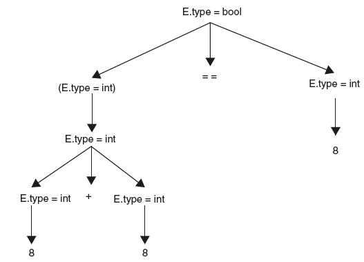
   Figure 6.8 Annotated Parse Tree for String “(8 + 8) = = 8”

6.4  Bottom-Up Evaluation of SDT

Given an SDT, we can evaluate attributes even during bottom-up parsing. To carry out the semantic actions, parser stack is extended with semantic stack. The set of actions performed on semantic stack are mirror reflections of parser stack. Maintaining semantic stack is very easy.

During shift action, the parser pushes grammar symbols on the parser stack, whereas attributes are pushed on to semantic stack.

During reduce action, parser reduces handle, whereas in semantic stack, attributes are evaluated by the corresponding semantic action and are replaced by the result.

For example, consider the SDT 

A → X Y Z

{A · a := f(X · x, Y · y, Z · z);}

The stack contents would be as shown in Figure 6.9.

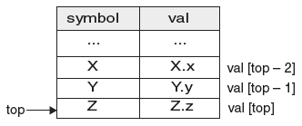
Figure 6.9 Stack Content While Parsing

Strictly speaking, attributes are evaluated as follows 

A → X Y Z

{val[ntop] := f(val[top - 2], val[top - 1], val[top]);}

 

Evaluation of Synthesized Attributes

• Whenever a token is shifted onto the stack, then it is shifted along with its attribute value placed in val[top].
• Just before a reduction takes place the semantic rules are executed.
• If there is a synthesized attribute with the left-hand side nonterminal, then carrying out semantic rules will place the value of the synthesized attribute in val[ntop].

Let us understand this with an example:

 

input string 7 * 7

Figure 6.10 shows the result of shift action. Now after performing reduce action by E → E * T resulting stack is as shown in Figure 6.11.

Along with bottom-up parsing, this is how attributes can be evaluated using shift action/reduce action.

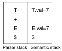
Figure 6.10 Stack Content While Parsing

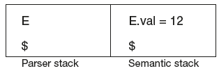
Figure 6.11 Stack Content After Reduction

* Example 4:

Consider the following SDT.

 

If an SR parser carries out the translations specified, immediately after reducing with rules of grammar, what is the result of carrying out the above translations on an input string “x⁴ y z²”?

Solution: Given an SDT, to trace out SDT on an input string, take the string and draw a parse tree. Now look at the order in which reductions are performed by the bottom-up parser. Whenever the parser reduces by rule, carry out the attached semantic action, that gives you the result. For the input string “xxxxyzz,” the parse tree is as shown in Figure 6.12

So here the first reduction is y to S, result is print (2). Next reduction is Sz to W, result of semantic action is print (3); next reduction is xxW to S, result is print(1); Next reduction is Sz to W, result of semantic action is print (3); next reduction is xxW to S, result is print(1);

So the final output is: 23131.

* Example 5:

Consider the SDT given below.

 

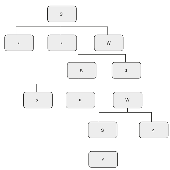
Figure 6.12 “xxxxyzz” Parse Tree

• Using the SDT construct parse tree and evaluate string 4 – 2 – 4 * 2
•  It is also required to compute the total number of reductions performed to parse the given input string. Modify the SDT to find the number of reductions.

Solution:

• To evaluate the expression, there are two ways. The simple method is to take the precedence and associativity of operators defined in the grammar. “–” has higher precedence than “*.” “–” is right associative and “*” is left associative. By considering this it can be evaluated without having the parse tree as follows:

        (4 – (2 – 4)) * 2 = 4 – (–2) * 2 = 12. 

  The second method is the blind method, that is, using the parse tree. Construct a parse tree for the expression that takes care of precedence and associativity. Evaluate the expression from the parse tree as shown in Figure 6.13.

  First evaluate inner sub tree (2 – 4) = –2. The next sub tree to be evaluated is 4 – (–2) = 6. The final sub tree to be evaluated is 6 * 2 = 12.

• Modifying SDT is similar to writing SDT. To find the number of reductions, one simple way is to use a global variable “count” and increment for every reduction. But this is not an advisable solution.

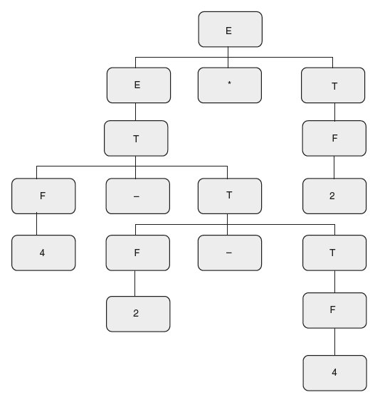
Figure 6.13 Parse Tree for “4 – 2 – 4 * 2”

Other alternative is to use an attribute ”red,” to keep track of the number of reductions. The advantage of taking the number of reductions as attribute is that we can store the number of reductions at any node in the parse tree with the attribute. Now let us see how to define semantic actions for evaluation of attribute .”red.”

Use the parse tree shown in Figure 6.13, traverse the parse tree, whenever any reduction is performed, define rule for finding number of reductions.

For example, the first reduction is reducing terminal “4” to F. So here the number of reductions performed is one. So whether “2” is reduced or “4” is reduced, the number of reduction is one. Hence, define semantic actions as follows:

 

	F → 2	{ F•val = 2; F•red = 1;}
	F → 4	{ F•val = 4; F•red = 1;}

 

The next reduction is F to T; when this is reduced, the number of reductions is the number of reductions at child node plus one. Hence, define semantic actions as follows:

 

T → F

{ T•val = F•val; T•red = F•red + 1;}

 

Similarly, for T to E, the same thing is applicable.

 

E → T

{ E•val = T•val; E•red = T•red + 1;}

 

The next reduction is F-T to T; when this is reduced, the number of reductions is the number of reductions at the left child plus the number of reductions at the right child plus one. Hence, define semantic actions as follows:

 

T → F – T

{ T•val = F•val – T•val; T•red = F•red + T•red + 1;}

 

Similarly, for E * T to E, the same thing is applicable.

 

E → E * T

{ E•val = E•val * T•val; E•red = E•red + T•red + 1;}

 

Hence, the final SDT after modifications is as follows:

 

	E → E * T	{ E•val = E•val * T•val; E•red = E•red + T•red + 1;}
	E → T	{ E•val = T•val; E•red = T•red + 1;}
	T → F – T	{ T•val = F•val – T•val; T•red = F•red + T•red + 1;}
	T → F	{ T•val = F•val; T•red = F•red + 1;}
	F → 2	{ F•val = 2; F•red = 1;}
	F → 4	{ F•val = 4; F•red = 1;}

 

The annotated parse tree for the input string “4 – 2 – 4 * 2” is shown in Figure 6.14.

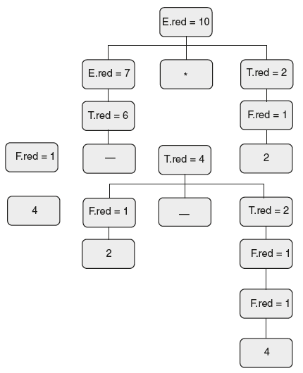
Figure 6.14 Decorated Parse Tree for “4 – 2 – 4 * 2”

Example 6:

Write an SDT to count the number of binary digits. For example, “1000” is 4.

Solution:

First define the grammar for a binary number. Binary digit “B” can be either “1” or “0.” The number can be a list of binary digits. The list can recursively define bits “B.” So grammar is as follows:

 

      N → L

      L → LB

      L → B

      B → 0

      B → 1

 

The next step is to take a small string and draw a parse tree. So take 1000 and draw a parse tree as shown in Figure 6.15.

The third step in SDT is to define semantic actions. Assume “count” as an attribute to count digits.

For example, the first reduction is the reducing terminal “1” to B. So here the number of digits, that is, the digit count is one. So whether “0” is reduced or “1” is reduced, the count is one. Hence, define semantic actions as follows:

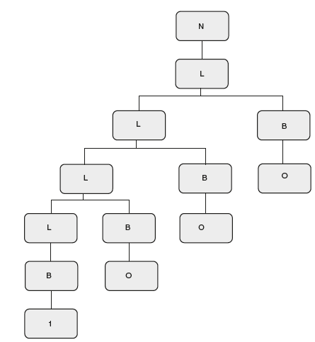
Figure 6.15 Parse Tree for “1000”

	B → 0	{ B•count = 1;}
	B → 1	{ B•count = 1;}

 

The next reduction is B to L; when this is reduced, the number of digits is the number of digits at the child node. Hence, define semantic actions as follows:

 

L → B

{ L•count = B•count;}

 

The next reduction is LB to L; when this is reduced, the count is the number of digits at the left child plus the count at the right child. Hence, define semantic actions as follows:

 

L → LB

{ L•count = L•count + B•count;}

 

Final SDT for counting the number of digits in a binary number is as follows:

 

	N → L	{ N•count = L•count;}
	L → LB	{ L•count = L•count + B•count;}
	L → B	{ L•count = B•count;}
	B → 0	{ B•count = 0;}
	B → 1	{ B•count = 1;}

Example 7:

Write an SDT to convert binary to decimal. For example, the binary number 101.101 denotes the decimal number 5.625.

Solution:

First define the grammar for a binary number. The binary digit “B” can be either “1” or “0.” The number can be a list of binary digits. The list can recursively define bits “B.” A binary number can be with decimal or without decimal. So the grammar is as follows:

 

      N → L₁•L₂

      N → L

      L → LB

      L → B

      B → 0

      B → 1

 

The next step is to take a small string and draw a parse tree. First, we consider a binary without decimal. So take 101.101 and consider only the left sub tree for 101. Draw a parse tree as shown in Figure 6.16.

The third step in SDT is to define semantic actions. Assume “dval” as an attribute to store the decimal equivalent of binary.

For example, the first reduction is the reducing terminal “1” to B. So here “dval” is one. If it is “0” decimal equivalent “dval” is 0. Hence, define semantic actions as follows:

 

	B → 0	{ B•dval = 0;}
	B → 1	{ B•dval = 1;}

 

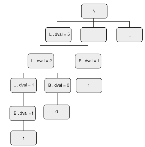
Figure 6.16 Parse Tree for “4 – 2 – 4 * 2”

The next reduction is B to L; when this is reduced, decimal equivalent “•dval” is whatever value the child node has. Hence, define semantic actions as follows:

 

L → B

{ L•dval = B•dval;}

 

The next reduction is LB to L; when this is reduced, the decimal equivalent “dval” is “dval” at the left child *2 plus “dval” at the right child. Hence, define semantic actions as follows:

 

L → LB

{ L•dval = L•dval * 2 + B•dval;}

 

The final SDT for converting a binary number without decimal to decimal equivalent is as follows:

 

	N → L1•L2	{}
	N → L	{ N•dval = L•dval;}
	L → LB	{ L•dval = L•dval * 2 + B • dval;}
	L → B	{ L•dval = B•dval;}
	B → 0	{ B•dval = 0;}
	B → 1	{ B•dval = 1;}

 

The annotated parse tree for string 101 is as shown in Figure 6.17.

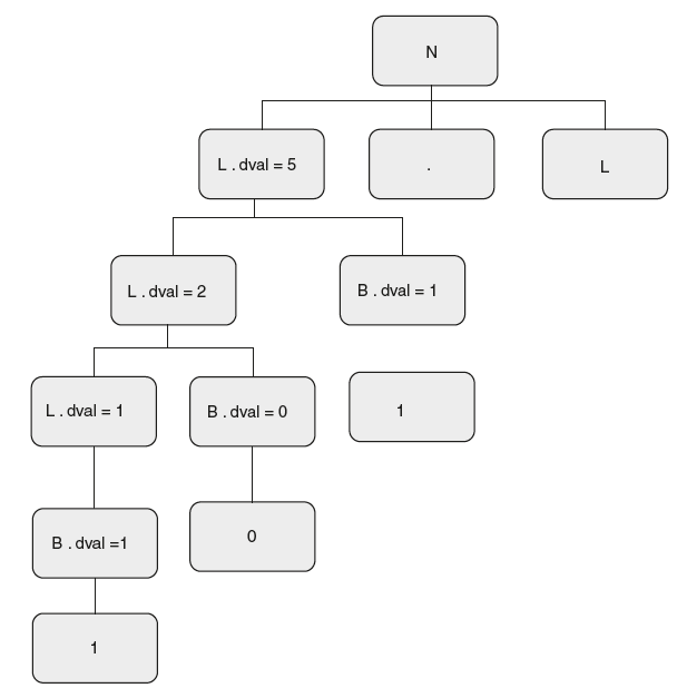
Figure 6.17 Annotated Parse Tree for “101”

Now let us extend the SDT for the decimal part. As we have already defined rules for the nonterminal L, given an input string 101•101, the defined semantic actions are carried out even for the right sub tree. This results in an equivalent for the decimal part, that is, 101 as 5. Now as this is already evaluated, we can get the decimal equivalent for the decimal part as follows:

L.dval/2^L.nd where “dval” is the decimal equivalent of the number after the decimal and “nd” is the number of digits after the decimal. For example, 101, dval = 5 and nd = 3.

So equivalent = 5/2³ = 5/8 = 0.625.

Let us now extend SDT for evaluating the number of digits “nd.” This is similar to the previous example of counting the number of digits in binary. So the final SDT is shown below:

 

	N → L1 • L2	{ N•dval = L1•dval + L2•dval / 2 L2•nd;}
	N → L	{ N•dval = L•dval;}
	L → LB	{ L•dval = L•dval * 2 + B•dval; L•nd = L•nd + B•nd;}
	L → B	{ L•dval = B•dval; L•nd = B•nd;}
	B → 0	{ B•dval = 0; B•nd = 1;}
	B → 1	{ B•dval = 1; B•nd = 1;}

6.5  Creation of the Syntax Tree

The parser produces a tree while checking the syntax of the programming language construct. This is called the parse tree. A parse tree gives the complete syntax of a string. It tells you what the syntax behind the string is. Hence it is called concrete syntax tree, whereas a condensed form of a parse tree is called syntax tree, which abstracts away unnecessary terminals and nonterminals. Hence, it is even called abstract syntax tree(AST).

For example, consider the string 3 * (4 + 2). The parse tree and syntax tree for the string are shown in Figure 6.18.

Now let us see how to write an SDT for creating a syntax tree.

Example 8:

SDT for creating a syntax tree

Solution:

Assume that an input string is of the form “a + b * c.”

The first step is to define grammar. Take unambiguous grammar that defines all arithmetic expressions with “+” and “*.”

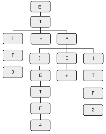
Figure 6.18 Parse Tree/Concrete Syntax Tree

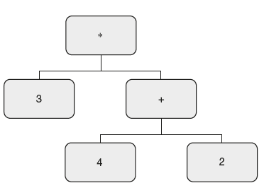
Syntax Tree/Abstract Syntax Tree

      E→E+T | T

      T→ T*F |F

      F→id

 

The second step is to take the input string and draw a parse tree. It is shown in Figure 6.19.

The third step is defining semantic actions. Here we are supposed to construct a node in the parse tree at any time. For creating a node, assume that there is a procedure mknode(l, d, r), where l is the left pointer, d is the data element, and r is the right pointer. Assume that when mknode() is called with three arguments, creates a node, and returns the pointer to the newly created node. Now let us see how the tree is created by using mknode().

The first reduction is identifier “a” is reduced to F. Here we need to create a leaf node. For creating leaf nodes we use the mknode() function with the left pointer and the right pointer as NULL. The return type of function is the pointer to the newly created node. So to store this node pointer, assume that there is an attribute “nptr.” The semantic action is as follows:

 

F → id

{ F•nptr = mknode ( NULL, id•lvalue, NULL );}

 

The next reduction is F to T. Here simply extend the pointer further to T by adding semantic action as

 

T → F

{ T•nptr = F•nptr;}.

 

Similarly, even for the next reduction T to E, extend the pointer further.

The next reduction is “T*F” to T. Here create a node using the mknode() function with “*” as data element and T•nptr as the left pointer and F•nptr as the right pointer as shown below:

 

T → T * F

{ T•nptr = mknode ( T•nptr, “*”, F•nptr );}.

 

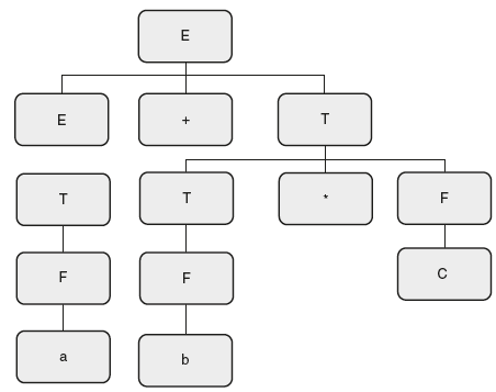
Figure 6.19 Parse Tree for “a + b * c”

 

The same thing can be carried out for E+T to E as

 

E → E + T

{ E•nptr = mknode ( E•nptr, “+”, T•nptr );}.

 

So the final SDT for creating syntax tree is as follows:

 

	E → E + T	{ E•nptr = mknode ( E•nptr, “+”, T•nptr );}
	E → T	{ E•nptr = T•nptr;}
	T → T * F	{ T•nptr = mknode ( T•nptr, “*”, F•nptr );}
	T → F	{T•nptr = F•nptr;}
	F → id	{ F•nptr = mknode ( NULL, id•lvalue, NULL );}

 

where mknode (l, d, r) is a function that creates a node with “l” as the left pointer and “d” as the data element, and “r” as the right pointer. It returns pointer to a newly created node.

The resulting syntax tree for input string “a + b * c” is as follows shown in Figures 6.19 and 6.20.

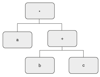
Figure 6.20 Syntax Tree for “a + b * c”

6.6  Directed Acyclic Graph (DAG)

DAG is used to identify common sub expressions. It helps us in eliminating redundant code.

For example, let there be an expression a + (b * c) + (b * c). This expression can be represented as tree or DAG as shown in Figure 6.21.

So here, for a common sub expression, a node is created twice in a tree, whereas in DAG, it is created only once and reused later. Now let us see how to write SDT for creating DAG, that is, for the above SDT, given an input string a+a*a, if we carry out the above translations, we get the syntax tree as found in Figure 6.22.

But we want DAG as shown in Figure 6.23.

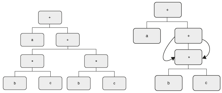
Figure 6.21 (a) Syntax Tree (b) DAG

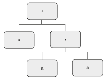
Figure 6.22 Syntax Tree for “a + a * a”

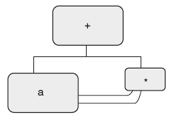
Figure 6.23 DAG for “a + a * a”

So to get a DAG, do we have to rewrite the SDT in Example 8 or do we have to modify the SDT? What changes are required, if any? No single change is required in SDT—Example 8. As it is, the same SDT can be used even for creating DAG but the difference is in function mknode(). Earlier, we have defined mknode() as function that when called blindly creates a node and returns a node. Now the modification required is in mknode(). Here, it should maintain a list of pointers already created.

Whenever mknode() is called, it first verifies whether the node is already created or not. If it is already created, return the same pointer. If it is not there in the already created node list, then it creates one and adds to list.

Example 9:

SDT for creating DAG

Solution:

 

	E → E + T	{ E•nptr = mknode ( E•nptr, “+”, T•nptr );}
	E → T	{ E•nptr = T•nptr;}
	T → T*F	{ T•nptr = mknode ( T•nptr, “*”, F•nptr );}
	T → F	{ T•nptr = F•nptr;}
	F → id	{ F•nptr = mknode ( NULL, id•lvalue, NULL );}

 

where mknode (l,d,r) function maintains a list of pointers already created. Whenever it is called, first it verifies whether the node is already created or not. If it is already created, return the same pointer. If it is not there in already created node list, then creates one and adds to list.

6.7  Types of SDTs

There is one more type called the L-attribute definition. The difference between S-attributed and L-attributed is as follows:

 

S-attributed definition	L-attributed definition
It uses only synthesized attributes. Semantic actions can be placed only at the end of the right hand side of a production. Attributes are generally evaluated during bottom-up parsing.	It allows both types. But if an inherited attribute is present, there is a restriction. The restriction is that each inherited attribute is restricted to inherit either from parent or from left sibling only. Semantic actions can be placed anywhere on the right hand side. Attributes are generally evaluated by traversing the parse tree depth first and left to right.

6.8  S-Attributed Definition

So far whatever the examples we have used is S-attributed definition only. Look at the examples; in all the examples, the type of attribute used, that is, “val” or “type” or “red” or “count” or “nptr” is only synthesized. A syntax-directed definition that uses synthesized attributes exclusively is said to be an S-attributed definition, where “S” stands for simple. S-attributed definition is also called postfix SDT as semantic actions are always placed only at the right end of productions.

6.9 Top-Down Evaluation of S-Attributed Grammar

So far we have seen bottom-up evaluation of S-attributed grammar, that is, given an SR/LR parser. If the translations are carried out, what would be the output? Suppose we have a top-down parser with SDT; can’t we carry out the same translations? Yes. We can carry out even by using the top-down parser. The difference is if it is bottom-up parser, we can easily specify when exactly the translation is carried out. For example, so far the assumption is that whenever the parser reduces by any production, the corresponding semantic action is carried out automatically, whereas with top-down parser, no doubt translations can be carried out. But we cannot tell when exactly the translations are carried out. So far we have seen enough examples for bottom-up evaluation. Now let us see some examples for top-down evaluation.

Given an SDT, a top-down parser carries out translations as follows:

1. Assumes semantic actions as dummy nonterminals, which become part of the right hand side of production.
2. Translations are pushed onto the stack along with grammar symbols.
3. When a dummy nonterminal appears on top of the stack, the terminal is popped and corresponding action is carried out.

To understand the above procedure, let us take a simple SDT

Example 10:

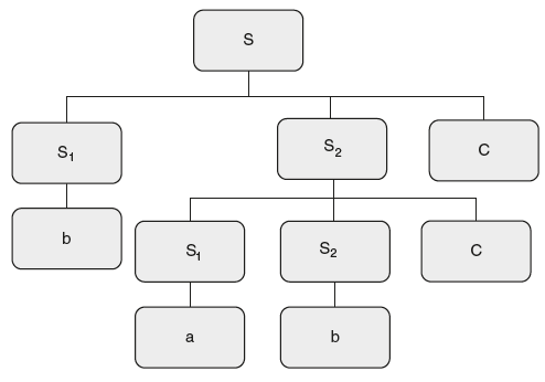
Write an SDT for counting the number of balanced parenthesis. For example, given ((())) should give 3 as output.

Solution: The grammar for balanced parentheses is as follows:

 

 

The second step is to draw the parse tree for an input string “((())).” It is shown in Figures 6.24 and 6.25.

The last step is to define the rules.

 

 

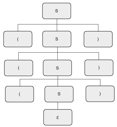
Figure 6.24 Parse Tree for Balanced Parentheses

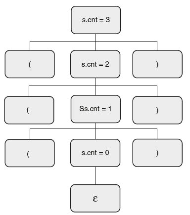
Figure 6.25 Annotated Parse Tree for “((())).”

The annotated parse tree is as follows:

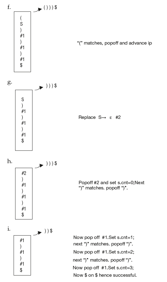
Top-down evaluation is as follows:

1. Assume semantic actions as dummy nonterminals.

    

   	S → ( S1 )	#1
   	| ε	#2
   	where #1	is S•cnt=S1•cnt+1;
   	and #2	is S•cnt=0;

2. Use LL(1) parsing algorithm to parse the input string.
3. During parsing if #1 or #2 appears on top of the stack, then take out the symbol and carry out the translations as shown in Figure 6.26.
   
   

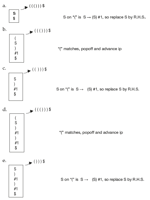
   Figure 6.26 Parser Actions in Top-Down Evaluation

This is how top-down evaluation of S-attributed definition can be carried out. Even observe that given an SDT whether it is top-down evaluation or bottom-up evaluation, the result is the same for the given input string.

6.10  L-Attributed Definition

1. It allows both types, that is, synthesized as well as inherited. But if at all an inherited attribute is present, there is a restriction. The restriction is that each inherited attribute is restricted to inherit either from parent or from left sibling only.

   For example, consider the rule

   A → XYZPQ assume that there is an inherited attribute, “i” is present with each nonterminal. Then,

   Z•I = f(A•i|X•i|Y•i) but Z•i = f(P•i|Q•i) is wrong as they are right siblings.

2. Semantic actions can be placed anywhere on the right hand side.

   Ex:	Ex: A → a{}
   	B → C {} D
   	C → EF {}

       They can be placed either in the beginning or in the middle of grammar symbols or at the end.

3. Attributes are generally evaluated by traversing the parse tree depth first and left to right. It is possible to rewrite any L-attributes to S-attributed definition.

Example 11:

Consider the following SDT:

 

	A → LM	{ L•i = f(A•i);
		M•i = f(L•s)
		A•s = f(M•s);}
	A → QR	{ R•i = f(A•i);
		Q•i = f(R•s)
		A•s = f(Q•s);}

 

Is it L-Attributed or S-Attributed?

Solution: Look at semantic actions. Here by looking at semantic actions we understand that “s” is synthesized and “i” is inherited. So actions in first rule are correct since “i” is dependent on parent or left siblings only. But look at the second action in A → QR, Q.i = f(R.s); this violates the basic property of L-attributed definition. Inherited attribute can inherit either from parent or from left sibling only. So this is a wrong SDT—not S-attributed or not L-attributed.

So far we have discussed enough examples for S-attributed definition. Now let us look at some examples for L-attributed definition.

Let us start with a simple example .Consider the S-attributed definition for converting infix to the post fix form.

 

Consider actions as dummy nonterminals #1,#2,#3.

      E → E₁ + T    #1

      E → T

      T → T₁ * F    #2

      T → F

      F → id    #3

 

Eliminate left recursion. Now we get simple L-attributed definition as follows:

Example 12:

L-attributed definition for converting infix to post fix form.

 

      E → TE”

      E” → +T #1 E” | ε

      T → F T”

      T” → * F #2 T” | ε

      F → id      #3

 

where #1 corresponds to printing “+” operator, #2 corresponds to printing “*,” and # 3 corresponds to printing id.val.

Look at the above SDT; there are no attributes, it is L-attributed definition as the semantic actions are in between grammar symbols. This is a simple example of L-attributed definition. Let us analyze this L-attributed definition and understand how to evaluate attributes with depth first left to right traversal. Take the parse tree for the input string “a + b*c” and perform Depth first left to right traversal, i.e. at each node traverse the left sub tree depth wise completely then right sub tree completely.

Follow the traversal in Figure 6.27. During the traversal whenever any dummy nonterminal is seen, carry out the translation.

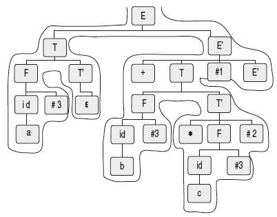
Figure 6.27 Depth First Traversal of Tree

• So if we follow the path, the first dummy nonterminal that is seen is #3 after seeing identifier “a.” So carryout #3, which results in printing out “a.”
• Next dummy nonterminal seen is #3 after seeing identifier “b.” So carryout #3, which results in printing out “b.”
• Next dummy nonterminal seen is seen is #3 after seeing identifier “c.” So carryout #3, which results in printing out “c.”
• Next dummy nonterminal seen is #2, which results in printing out “*.”
•  The last dummy nonterminal seen is #1, which results in printing out “+.”
• So the final result is “abc*+.”

Let us take another example of L-attributed with attributes.

Example 13:

Write an SDT for storing type information in a symbol table.

Solution:

Given an input string int a,b,c, the SDT should give an output as

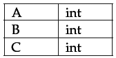
The first step is to define grammar for declaration statements of the form int a,b,c

 

      D → TL

      T → int

      T → char

      L → L, id

      L → id

 

The second step is to take the input string and draw a parse tree as shown in Figure 6.28.

The third step is to define semantic actions. Here, the parser first reads “int” and reduces to T. So to store the type information, assume an attribute “type” with a grammar symbol and store the type by defining semantic actions as follows:

 

	T → int	{ T•type = int}
	T → char	{ T•type = char}

 

The resulting parse tree is as shown in Figure 6.29.

Now look at the parse tree; type information is available at node T, whereas node L is deriving identifiers a, b, c. So if the type information at node T is made available with node L then whenever an identifier is seen, it stores type together with identifier. Now the question is how to propagate type information from node T to node L. Can we write semantic action as follows?

 

D → TL

{L•type = T•type;}

 

Is this correct? No. “type” is a synthesized attribute; so using synthesized attribute we cannot propagate information to sibling. So the only way here is to use an inherited attribute.

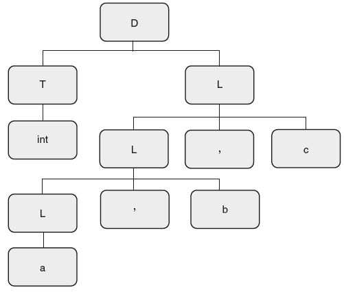
Figure 6.28 Parse Tree for “int a, b, c”

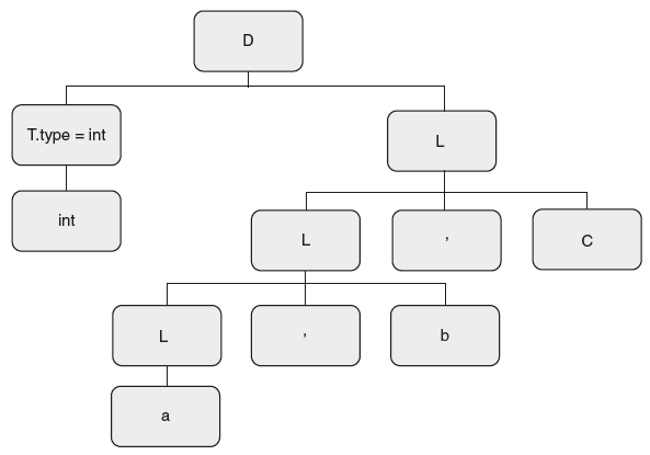
Figure 6.29 Propagating Type Info in Parse Tree

Assume that there is an inherited attribute “in.” Now we can define the rule as follows:

 

D → TL

{L•in= T•type;}

 

As “in” is an inherited attribute, it can take type information from node T.

Now node L takes type information from T. Now child L takes type info from parent using inherited attribute by having action as

 

L → L1, id

{ L1•in = L•in;}.

 

Now type is available with L and id is also available. Assume add_type(type,id) as a function that stores id together with type into symbol table. So add the action as follows:

 

L → L1, id

{ L1•in = L•in; add_type(L1•in, id);}.

 

Finally, when id is reduced to L, we have type information together with id, so store it in symbol table by defining rule as

 

L → id

{ add_type(L•in, id•name);}

 

So the final SDT is as follows:

 

	D → TL	{L•type = T•type;}
	T → int	{ T•type = int}
	T → char	{ T•type = char}
	L → L1, id	{ L1•in = L•in; add_type(L1•in, id);}
	L → id	{ add_type(L•in, id•name);}

 

The annotated parse tree is as shown in Figure 6.30.

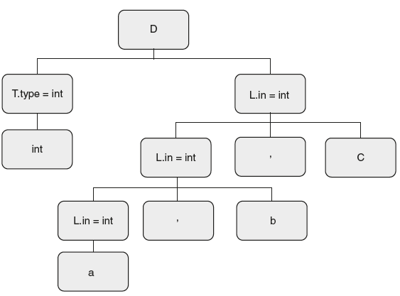
Figure 6.30 Depth First Traversal of Tree

This is an L-attributed definition that uses both synthesized and inherited attributes.

General evaluation of semantic actions in any SDT is as follows:

1. Take input string, parse it, and it gives parse tree.
2. Traverse the parse tree and draw the dependency graph.
3.  Graph gives evaluation order.

Let us understand the procedure with the above example.

Take the parse tree and dependency graph. Dependency graph is a graph that shows inter dependencies among the attributes. The dependency graph is shown below in Figure 6.31.

We follow the dependency graph that gives you the evaluation order.

The evaluation order is as follows:

 

      a1 = int

      a2 = a1

      a3 = a2

      add_type(int,a)

      a4 = a3

      add_type(int,b)

      add_type(int,c)

 

The general procedure is complex. Hence, we have discussed specific procedures. The simple procedures are if it is S-attributed, evaluate during bottom-down parsing. If it is L-attributed, traverse the parse tree depth first left to right.

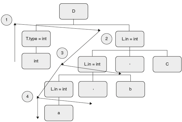
Figure 6.31 Dependency Graph

Let us see how to evaluate attributes by traversing parse tree depth first left to right. Depth first left to right traversal is at each node traverse the left sub tree depth wise then right sub tree completely. During this traversal evaluate attributes as follows:

•  Evaluate inherited attributes if the node is visited for the first time
• Evaluate synthesized attributes if the node is visited for the last time

Look at Figure 6.32. Start at point 1; here node D has no attributes defined. So continue till 2. Here node T is visited for the first time; so evaluate inherited attributes. Node T is not defined with any inherited attributes, so continue till point 3. At 3, it is the last visit for node T, so evaluate synthesized attributes T → int {T.type = int}. So node T will have type information. Now continue till point 4; at 4, the first visit for node L, evaluate inherited attribute {L.in=T.type;}. Node L, at point 5 is the first visit, so evaluate inherited.

L → L₁, id { L₁.in = L.in; add_type(L₁.in, id);} Here add_type() has two arguments—L.in, which is inherited attribute and ‘id‘ is synthesized attribute. As function has both types of attributes, it can be evaluated only at the last visit. Similarly, at point 6, the inherited attribute is evaluated. Now at point 7, the last visit, so add_type() is carried out with the result, “a” with type “int” is stored in symbol table. Now at point 8, the last visit, add_type() is carried out with the result, “b” with type “int” is stored in symbol table. Now at point 9, the last visit, add_type() is carried out with the result, “c” with type “int” is stored in the symbol table. At point 10, it completes traversal. By this time a,b,c, along with type is stored in the symbol table.

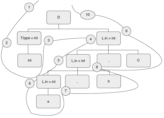
Figure 6.32 Depth First Left to Right Traversal of Tree

6.11  Converting L-Attributed to S-Attributed Definition

Now that we understand that S-attributed is simple compared to L-attributed definition, let us see how to convert an L-attributed to an equivalent S-attributed.

Consider an L-attributed with semantic actions in between the grammar symbols. Suppose we have an L-attributed as follows:

 

      S → A {} B

 

How to convert it to an equivalent S-attributed definition? It is very simple!!

Replace actions by nonterminal as follows:

 

      S → A M B

      M → ε            {}

Example 14:

Convert the following L-attributed definition to equivalent S-attributed definition.

 

	E → TE”
	E” → +T	#1 E” | ε
	T → F T”
	T” → *F	#2 T” | ε
	F → id	#3

Solution:

Replace dummy nonterminals that is, actions by nonterminals.

 

Example 15:

Consider Example 13; let us see how to convert L-attributed to equivalent S-attributed definition.

Solution:

To get the equivalent S-attributed definition, we need to eliminate inherited attributes in Example 13. How to avoid inherited attributes in Example 13? Recollect Example 13, there as type information is to be taken from node L which is a sibling, the only way is using inherited attribute. So as long as we use that grammar, L will be a sibling to T. As long as L is sibling to T, inherited attribute is needed. So to avoid inherited attribute the only way is to rewrite the grammar as follows:

 

      D → D₁, id

      D → T, id

      T → int | char

 

The parse tree for the string int a,b,c is as shown in Figure 6.33.

Now define the semantic actions as follows:

First read “int” then reduce “int” to T. So to store type, assume attribute type and define rule as

 

T → int

{T•type = int}

 

Next it reads “a,” then reduces ‘T id’ to D. So here we propagate type information to parent by using the same synthesized attribute and also store type with id into symbol table by using add_type() by defining semantic action as follows:

 

D → T, id

{L•type = T•type; add_type(T•type, id•name)}

 

Next it reads “b,” then reduces ‘D, id’ to D. So here we propagate type information to parent by using the same synthesized attribute and also store type with id into symbol table by using add_type() by defining semantic action as follows:

 

D → D1, id

{D•type = D1•type; add_type(D1•type, id•name);}

 

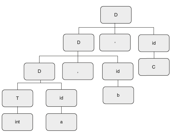
Figure 6.33 Parse Tree for “int a, b, c”

So the final equivalent L-attributed definition is as follows:

 

	D → D1, id	{D•type = D1•type; add_type(D1• type, id•name);}
	D → T, id	{L•type = T•type; add_type(T•type, id•name)}
	T → int	{T•type = int}
	T → char	{T•type = char}

 

So to convert L-attributed to equivalent S-attributed here, grammar is changed. But rewriting grammars is not a simple solution. Consider the following example SDT:

A → BC {A•i=B•i + C•i;} is S-attributed and also L-attributed since there are no inherited attributes. So every S-attributed is even L-attributed. However, the reverse is not true.

6.12  YACC

YACC—Yet Another Compiler Compiler—is a tool for construction of automatic LALR parser generator.

Using Yacc

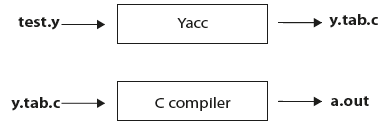
Yacc specifications are prepared in a file with extension “.y” For example, “test.y.” Then run this file with the Yacc command as “$yacc test.y.” This translates yacc specifications into C-specifications under the default file mane “y.tab.c,” where all the translations are under a function name called yyparse(); Now compile “y.tab.c” with C-compiler and test the program. The steps to be performed are given below:

Commands to execute

$yacc test.y

This gives an output “y.tab.c,” which is a parser in c under a function name yyparse().

With –v option ($yacc -v test.y), produces file y.output, which gives complete information about the LALR parser like DFA states, conflicts, number of terminals used, etc.

 

      $cc y.tab.c

      $./a.out

Preparing the Yacc specification file

Every yacc specification file consists of three sections: the declarations, grammar rules, and supporting subroutines. The sections are separated by double percent “%%” marks.

 

        declarations

      % %

        Translation rules

      % %

        supporting subroutines

 

The declaration section is optional. In case if there are no supporting subroutines, then the second %% can also be skipped; thus, the smallest legal Yacc specification is

 

      % %

        Translation rules

Declarations section

Declaration part contains two types of declarations—Yacc declarations or C-declarations. To distinguish between the two, C-declarations are enclosed within %{ and %}. Here we can have C-declarations like global variable declarations (int x=l;), header files (#include....), and macro definitions(#define...). This may be used for defining subroutines in the last section or action part in grammar rules.

Yacc declarations are nothing but tokens or terminals. We can define tokens by %token in the declaration part. For example, “num” is a terminal in grammar, then we define

% token num in the declaration part. In grammar rules, symbols within single quotes are also taken as terminals.

We can define the precedence and associativity of the tokens in the declarations section. This is done using %left, %right, followed by a list of tokens. The tokens defined on the same line will have the same precedence and associativity; the lines are listed in the order of increasing precedence. Thus,

 

      %left ‘+’ ‘-’

      %left ‘*’ ‘/’

 

are used to define the associativity and precedence of the four basic arithmetic operators ‘+’,‘-’,‘/’,‘*’. Operators ‘*’ and ‘/’ have higher precedence than ‘+’ and and both are left associative. The keyword %left is used to define left associativity and %right is used to define right associativity.

Translation rules section

This section is the heart of the yacc specification file. Here we write grammar. With each grammar rule, the user may associate actions to be performed each time the rule is recognized in the input process. These actions may return values, and may obtain the values returned by previous actions. Moreover, the lexical analyzer can return values when a token is matched. An action is defined with a set of C statements. Action can do input and output, call subprograms, and alter external vectors and variables. The action normally sets the pseudo variable “$$” to some value to return a value. For example, an action that does nothing but return the value 1 is { $$ = 1;}

To obtain the values returned by previous actions, we use the pseudo-variables $1, $2, . . ., which refer to the values returned by the grammar symbol on the right side of a rule, reading from left to right. Thus, if the rule is

A: BCD

for example, then $1 has the value returned by B, and $2 the value returned by C. As an example, consider the rule

 

      E: ’(’ E ’)’;

 

The value returned by this rule is usually the value of the E in parentheses. This can be indicated by

 

      E : ’(’ E ’)’ { $$ = $2;}

Lexical Analysis

The user must supply a lexical analyzer to read the input stream and communicate tokens (with lexeme values, if desired) to the parser. This can be done in two ways—either the lex tool can be used or a user can write his own hand-coded lexical analyzer in C. The lexical analyzer is an integer valued function with a default name “yylex().” The yylex() function returns an integer, which is the token number, representing the kind of token that is read. If there is a value associated with that token, it should be assigned to the yacc-defined global variable “yylval.” The parser and the lexer must agree upon these token numbers so that communication can take place between them. The numbers may be chosen by Yacc or by the user. In either case, These numbers are symbolically returned by the lexical analyzer by using the “# define” macro mechanisms of C.

For example, suppose that the token name NUM has been defined in the declarations section of the Yacc specification file.

 

The above code is to return a token NUM along with its value on seeing a digit. The value of token is equal to the numerical value.

If the lexical analyzer is supplied with the lex tool, first prepare the lex file like test.l. Run under lex. That gives you the “lex.yy.c” file. Add this as the first statement in supporting routines part as follows:

 

      % %

 

      % %

 

#include “lex.yy.c”

---------

When Yacc is invoked with the -v option (verbose), a file called y.output is created with complete description of the parser. The y.output file corresponds to the above grammar with a full description of the LALR parser.

Yacc invokes two disambiguating rules by default:

1. In case of a shift/reduce conflict, the default action is to go with the shift action.
2.  In case of a reduce/reduce conflict, the default action is to reduce action by the earlier grammar rule.

Supporting routines section

When a user prepares input a specification file to Yacc with “y” extension, it creates an output file called y.tab.c. An integer valued function “yyparse()” is produced by Yacc; when yyparse() is called, in turn it calls yylex(), which is the lexical analyzer supplied by the user to obtain input tokens. yyparse() returns the value 1 on error and returns 0 on EOF. The user must provide some supporting routines for this parser. For example, as with every C program, a program called “main” must be defined, that eventually calls parser function yyparse(). In addition to this, a routine called yyerror()is also required as it gives error diagnostics when a syntax error is detected. These two routines are compulsory for any yacc program. Consider the following example:

 

The argument to yyerror() is a string “str” containing an error message. The default stack type in YACC is integer type. If we want to change the stack type, we can overload stack definition using %union as follows:

 

This declares the Yacc value stack, and the global variables yylval. If Yacc was invoked with the -d option, the union declaration is copied onto th e y.tab.h file.

Using ambiguous grammars

When ambiguous grammar is used in translation rules, we get conflicts. So to resolve conflicts, we need to supply precedence and associativity of operators using %left.... %right... For example, when ambiguous grammar is given,then specifying following:

 

Indicates that *,/ has higher precedence than +, – and are left associative.

Error recovery with YACC

In YACC, error recovery is performed using error production. We add extra productions for taking care of errors as follows:

 

Errors (sent by lexical analyzer as error tokens) are parsed using the second rule shown in the above grammar. So when an error is captured, the error message “Enter last line once again” will appear, “yyerrok” is a yacc-defined macro that resets parser to its normal mode of operation. Let us have an example:

Example 16:

Write a YACC program for evaluation of expression like “8*8+8.”

Solution:

If we want to use hand coded yylex() for lexical analyzer with yacc, first prepare a YACC file “test.y” as follows:

Yacc program

 

To run the above program, execute the commands as follows:

 

If we want to use the “lex tool” instead of hand-coded yylex(), then first prepare the lex file “test.l” as follows:

Lex program

 

Let us use the lex tool with ambiguous grammar. The yacc program “test.y is as follows:

 

To run the above program, execute the commands as follows:

 

Solved Problems

1. Consider the following SDT. If an LR parser carries out the translations on an input string “aabbccdb,” what is the output?

	S → aaS	{ print(“a” );}
	| bA	{ print(“b” );}
	| b	{ print(“c” );}
	A → bcA	{ print(“d” );}
	| cdS	{ print(“e” );}

 

Solution: Take the input string; draw the parse tree

The first reduction is “b to S.” When this is reduced, the corresponding semantic action is print(“c” );

The next reduction is “cdS” to A. When this is reduced, the corresponding semantic action is print(“e” );

The next reduction is “bcA” to A. When this is reduced, the corresponding semantic action is print(“d” );

The next reduction is “bA” to S. When this is reduced, the corresponding semantic action is print(“b” );

The final reduction is “aaS” to S. When this is reduced, the corresponding semantic action is print(“a” );

Hence the final result is the string “cedba” is printed.

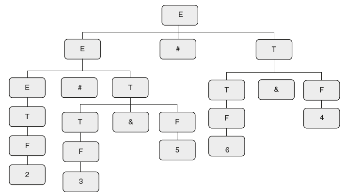
*2. Consider the SDT given below.

 

	E → E # T	{ E•val = E•val * T•val;}
	E → T	{ E•val = T•val;}
	T → T&F	{ T•val = T•val + F•val;}
	T → F	{ T•val = F•val;}
	F → num	{ F•val = num•val;}

 

What is the output for an input “2#3&5#6&4”?

Solution: Draw the parse tree for the string “2#3&5#6&4” as follows:

Here, look at semantic actions, “&” is used for addition and “#” is used for multiplication.

So the given string can be reduced as follows after replacing “&” by “+” and “#” by “*.”

 

      2 * 3 + 5 * 6 + 4.

 

If you look at the grammar, “+” has higher precedence than “*” and both are left associative.

Hence, the given string is evaluated as follows:

 

      2 * (3 + 5) * (6 + 4) = 2 * 8 * 10 = 160.

*3. Consider the SDT shown below

 

Convert it to S-attributed; then check if an LR parser carries out translation on an input “9+5+2” ; what is the output?

Solution:

Equivalent S-attributed definition is

 

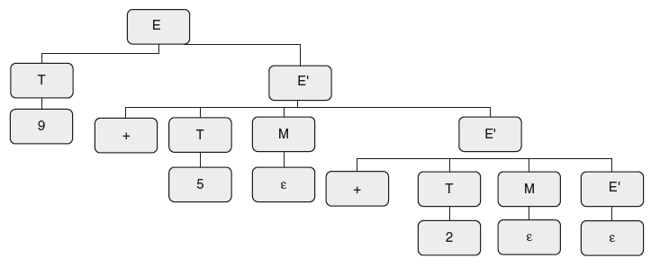
Draw a parse tree

Now evaluate from the parse tree. The first reduction is 9 to T. So prints 9.

Next is 5 to T, so prints 5. Next ε to M, prints +. Next reduction is 2 to T, prints 2.

Next ε to M, prints +. Next £ to E”, no action.

Final result is 95+2+.

 

4. Convert the following SDT

 

 

to an SDT that is postfix SDT and has no left recursion in underlying grammar.

Solution:

First eliminate left recursion. The resulting grammar is as follows:

 

To get postfix SDT, move actions at right end as follows:

 

 

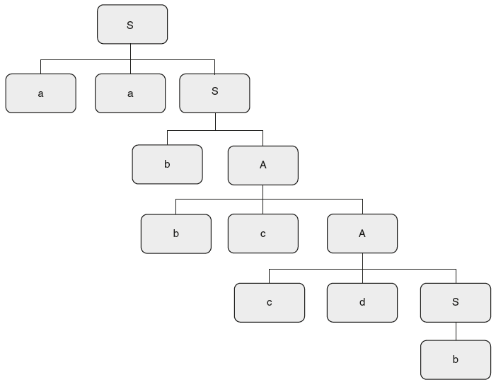
5. Consider the following SDT. If an LR parser carries out the translations on an input string “babcc.” What is the output?

 

	S → S1S2c	{S.t= S1.t-S2.t;}
	| a	{ S.t=5;}
	| a	{ S.t=2;}

 

    Solution: Draw a parse tree and carry out the translations.

    When “b” is reduced to S, result is s.t = 2.

    Next when “a” is reduced to S, result is s.t = 5.

    Next when “b” is reduced to S, result is s.t = 2.

    Next when “SSc” is reduced to S, result is 0.3

    Last when “SSc” is reduced to S, result is –1.  

Summary

• Grammar together with semantic actions is called syntax-directed translation.
• If the value of an attribute at a node is computed from the values of attributes at the children of that node in the parse tree then it is called synthesized attribute.
• If the value of an inherited attribute is computed from the values of attributes at the siblings or parent of that node.
• The parse tree that shows attribute values at each node is called annotated or decorated parse tree
• Parse tree is even called concrete syntax tree
• An SDT that uses only synthesized attributes is called S-attributed definition.
• An L-attributed definition allows both types. But if an inherited attribute is present there is a restriction. The restriction is that each inherited attribute is restricted to inherit either from parent or from left sibling only.
• Every S-attributed is even L-attributed.
• We can convert an L-attributed definition to equivalent S-attributed definition.
• S-attributed definition is also called postfix SDT.

Fill in the Blanks

1. Consider the SDT given below.

   S → aSb	{ S.count = S.count + 2;}
   | bSa	{ S.count = S.count + 2;}
   | ε	{ S.count = 0;}

   This SDT checks __________.

2. The other name of S-attributed definition is __________.
3. In SDT, A → BC {C.s = B.s;} attribute .“s” is __________.
4. Every L-attributed is S-attributed (Yes/No) __________.
5. An attribute that is evaluated in terms of attributes of its parent is called __________.
6. In___________SDD, semantic actions are placed anywhere on the right hand side.
7. Every S-attributed is L-attributed (Yes/No) __________.
8. We cannot convert an L-attribute definition to S-attributed definition. (Yes/No)
9. In SDT, A → BC {A.i = B.i;} attribute “i” is __________.
10. The interdependencies among attributes are shown by the __________ graph.

Objective Question Bank

1. Consider the SDT given below.

   	E → E+ T | T	{ count = count + 5; print ( count);}
   	T → T*F I F	{ count = count * 5;}
   	F → i	{count = 10;}

   What is the count after parsing the string “i + i * i” ?

   • 110
   • 55 
   • 550
   • 11
2. The SDT, A → BC {C.s = B.s;} is __________.
   • S-attributed 
   • L-attributed
   • both 
   • none
3. The SDT, A → BC {A.i = B.i;} is __________.
   • S-attributed 
   • L-attributed 
   • both 
   • none
4. The SDT, A →BC {B.s = C.s;} is __________.
   • S-attributed
   • L-attributed
   • both 
   • none
5. An S-attributed definition can be evaluated __________.
   • Top down 
   • bottom up 
   • both
   •  none

Key for Fill in the Blanks

1. total number of a’s and b’s
2.  postfix SDT
3.  Inherited
4.  N
5.  inherited
6.  L-attributed definition
7.  Y
8.  N
9. synthesized
10. dependency

Key for Objective Question Bank

1. b
2. b
3. c
4. d
5. c