

In this chapter we look at all things that move. Visual effects shots invariably entail some animation on the part of the digital compositor so an understanding of animation and how it works is essential. The subject of animation in this chapter is examined from several angles. First is a look at transforms, those operations in digital compositing that reposition or change the shape of an image. The affect of transforms on image quality and how pivot points affect the results of a transform are explained. There is also a section on different keyframe strategies and some advice on when to use which one.
Motion tracking and shot stabilization are pervasive parts of today’s visual effects shots so insight into their internal workings and tips on what to watch out for are offered. Both point trackers and planar trackers are covered. A close cousin of motion tracking is the match move, so there is some good information about how it works even though it is really a 3D thing. Finally, there is an extensive tour of different types of image warping techniques and when to use them, followed by the granddaddy of all warping techniques, the morph.
8.1 TRANSFORMS AND PIXELS
Transforms change the size, shape, or position of an image, which we do a lot in digital compositing. There are several different transforms, each with its own issues to be aware of. One issue to be aware of for all transforms is that they soften the image, as if a light blur had been applied. Even the simplest transform, such as a move, softens the image. Why this is so can be understood with the help of the little sequence starting in Figure 8-1 which shows a closeup of the nice sharp corner of a blue object on a red background. Let us assume the blue object is moved (translated) to the right by 0.7 pixels and shifted up by 0.25 pixels, illustrated with the aid of the arrow in Figure 8-2. The corner of the blue object now straddles the pixel boundaries represented by the black lines. However, this is not permitted. All pixels must stay within the pixel boundaries. It’s a rule.
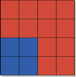
Figure 8-1 Sharp corner
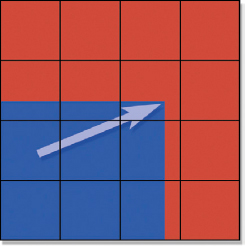
Figure 8-2 Moved
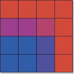
Figure 8-3 Averaged
To accommodate this awkward situation the computer now performs a simulation of how the picture would look if it were shifted a fraction of a pixel up and over and now straddles the pixel boundaries. The way it simulates this is by averaging the blue and red pixels together to create a new color based on the fraction of the red pixel that they cover.
Since the top row of blue pixels in Figure 8-2 moved up by 0.25 they now cover 25% of the red pixels so the averaged pixels in the top row of Figure 8-3 are 25% blue and 75% red. The right edge of the blue pixels moved over by 0.7 covering 70% of the red ones so in the averaged version those pixels are 70% blue and 30% red. After the upper right corner blue pixel is moved it covers 15% of its red pixel so the averaged pixels are 15% blue and 85% red. The effect of all this when seen from a normal viewing distance is that the edge of the blue object is no longer sharp. If you ran a gentle blur on the original image in Figure 8-1 the results would look very much like the translated version in Figure 8-3.

Figure 8-4 Translation

Figure 8-5 Rotation

Figure 8-6 Scale
We have just seen how a move (translation) softens an image. The same thing happens with the rotate transform in Figure 8-5. The rotated pixels straddle the pixel boundaries and must be averaged just like the translation pixels. There is one exception. Some programs have a “cardinal” rotate where the image can be rotated exactly 90 or 180 degrees. In these special cases the pixels are not averaged because the computer is simply remapping the pixel’s locations to another exact pixel boundary. No pixel averaging, no softening. Photoshop thoughtfully supports these special cases separately from their Edit > Transforms > Rotate by offering a separate choice for exactly 90 and 180 degree rotations as well as flip horizontal (otherwise known as a flop) and flip vertical.
The scale transform (Figure 8-6) is particularly hard on images when they are scaled up. One pixel might be stretched to cover one and a half or two pixels or more, which seriously softens the image. Generally speaking, you can scale an image up by about 10% before you start noticing the softening. Conversely, scaling an image down can increase its apparent sharpness. And don’t think that if an image is softened during a transform that you can restore the sharpness by reversing the transform. Because you can’t.
The skew transform (known by some as a shear) is shown Figure 8-7. The left example is skewed horizontally, which slides the top or bottom edges left or right. The right example is skewed vertically, which slides the left and right edges up and down.
Figure 8-8 shows a couple of examples of a four-corner pin, very popular for those ever-present monitor screen replacement shots. The four-corner pin is like attaching the image to a sheet of rubber, then pulling on the corners of the rubber. By tracking the four corners to the corners of a monitor the picture on the screen can be replaced. The skew and corner pin transforms can severely deform an image, introducing a lot of softening. To prevent this, a high-resolution version of the image can be transformed, and then the results scaled down to a smaller size to reintroduce its sharpness.

Figure 8-7 Skew/shear

Figure 8-8 Corner pin
As we have seen, transforms soften images except in the special case where the image is being scaled down. Then they are sharpened. So what happens if you string several transforms in a row? The image gets progressively softer with each transform. The fix for this is to combine or concatenate all of your transforms into a single complex transform so that the image only takes one softening hit. Most compositing programs have this feature. For example, if you have a move transform followed by a rotate followed by a scale, replace them all with a single MoveRotateScale transform.
In the pixel-softening alert above we saw how softening occurred because the pixel values were averaged together. However, averaging the pixel values is only one of several possible ways of calculating the new pixels. There are a variety of algorithms that might be used, and these algorithms are called filters. Change the filter and you change the appearance of the transformed image. Many compositing programs offer the option to choose filters with their transforms, so an understanding of how different filters affect the appearance of the transformed image is important. Also, choosing the wrong filter can introduce problems and artifacts, so being able to recognize these is also important. We will not be looking at how they work internally as the math is complex and irksome.
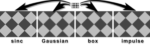
Figure 8-9 The effects of different filters
Figure 8-9 illustrates the effect of four filters commonly used for scaling up an image. The small checker pattern at the top was scaled up by a factor of 5 using a different filter in each example. The sinc filter on the left adds image sharpening in an attempt to avoid softening the resulting image. It does look sharper than the one next to it, but note the odd dark lines along the inside edge of the dark squares and the light lines along the inside edges of the light squares. This is an artifact of the image sharpening and can be objectionable under some circumstances. If you see this in a resized image and want to eliminate it, then switch filters.
The Gaussian filter does not attempt edge sharpening so it has no edge artifacts, but does not appear as sharp as the sinc filter. The box filter is not as soft as the Gaussian filter, but the jagged pixels of the original small image are starting to show. The impulse filter is jaggiest of them all because it is not really performing a filter operation. It is just replicating pixels from the smaller image using the “nearest neighbor” principle. It is also the fastest, so it is frequently used when the need is to increase the size of an image quickly such as for an interactive display—like your compositing program’s image viewer, for example.
The scale, rotate, and skew transforms have an additional feature that other transforms do not, and that is a pivot point. The pivot point is the center point around which all of the transform action takes place. Some call this an axis, others call it a center, and still others call it the anchor point. If we want to rotate something in the real world we don’t need a pivot point. We just grab it and rotate it. The computer, however, must be told where to locate the pivot point for a rotation because the pivot point’s location dramatically affects the results. And that is the point about the pivot point.

Figure 8-10 Pivot point centered
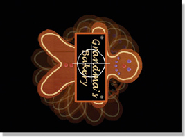
Figure 8-11 Rotate
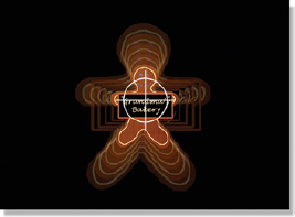
Figure 8-12 Scale
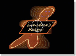
Figure 8-13 Skew
Let us consider two cases—one where the pivot point is in the center of the image and the other where it is well off-center. The centered pivot point can be seen in Figure 8-10 as the white cross-hair mark looking a bit like the sights of a high-powered rifle centered on the gingerbread man. The rotate, scale, and skew in Figure 8-11, Figure 8-12, and Figure 8-13 do exactly what we might expect of those transforms. No surprises here.
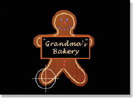
Figure 8-14 Pivot point off-center
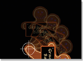
Figure 8-15 Rotate
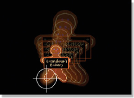
Figure 8-16 Scale
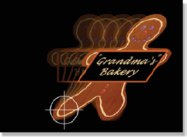
Figure 8-17 Skew
The second case in Figure 8-14 has the pivot point located well off-center in the lower left corner of the frame on the gingerbread man’s foot. The results are quite surprising. The rotate in Figure 8-15 has rotated the gingerbread man almost out of frame. The scale in Figure 8-16 has shifted it away from the center of frame. The skew in Figure 8-17 has shifted it towards the right edge of frame and with any more skew it will get cut off.
All of this illustrates the importance of the proper location for the pivot point of a transform. The default location will normally be the center of frame, which will usually be what you want. But all compositing systems offer the ability to move the pivot point around and even to animate its position. In fact, this is the source of most pivot point problems. What can happen is that the pivot point becomes shifted without you noticing it, then you perform a rotate, for example, and your gingerbread man disappears out of frame. Tip—always know where your pivot points are.
(To see a movie of the affect of the pivot point download www.compositingVFX.com.mov/CH08/Figure 8-14.)
(Download www.compositingVFX.com/CH08/gingerbread man.tif to try various transformations with different pivot points.)
8.4 TRANSFORMATION ORDER
The previous section showed how moving the pivot point around dramatically affected the results of various transformations. There is another issue that will affect the results of your transformations and that is the order that they are done.
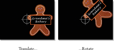
Figure 8-18 Translate followed by rotate
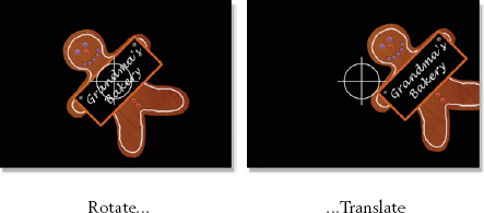
Figure 8-19 Rotate followed by translate
Figure 8-18 shows the results of just two transformations—a translate followed by a rotate. Mr. Gingerbread ended up in the upper right-hand corner after the rotate because he was off-center when the rotate was done using the pivot point in the middle of the screen.
Figure 8-19 shows the very different results of the same two transformations simply by reversing their order. In this example the rotate was done first followed by the translate. Mr. Gingerbread is now on the far right of the screen with one foot out of frame.
The point of this story is that if you have more than one transform operation in your compositing script, and then later change their order, you can expect your elements to suddenly shift position, which is usually a bad thing. Many compositing programs have a “master transform” operation that will incorporate the three most common transforms all together—translate, rotate, and scale—which is also the customary order of the transformations, and is often abbreviated “TRS.” Most will also have an option to change the order of the transformations from TRS to, say, STR (Scale, followed by Translate, followed by Rotate). Again, be sure to set the transformation order before you spend time positioning your elements so they don’t suddenly pop to a new location if reordered after the fact.
8.5 KEYFRAME ANIMATION
When it comes time to move things around on the screen, or create animation, the computer is your best friend. An image can be placed in one position on frame 1, moved to a different position on frame 10, and then the computer will calculate all of the in-between frames for you automagically. Frame 1 and frame 10 are known as the keyframes, so the computer uses these positions to calculate a new position for the image for each frame between frames 1 and 10. The calculations used by the computer to determine the in-between frames are called interpolation.
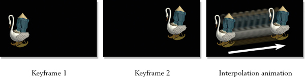
Figure 8-20 Simple keyframe animation
Figure 8-20 illustrates a simple keyframe animation. The classic CGI swan with a tent on her back was first positioned at frame 1 of the animation, which becomes keyframe 1. The frame counter was moved to frame 10 and the swan was positioned at keyframe 2. The computer now has two keyframes: one at frame 1 and the other at frame 10. When the animation is played back from frame 1 to 10 the computer interpolates the animation for all 10 frames. Nice.
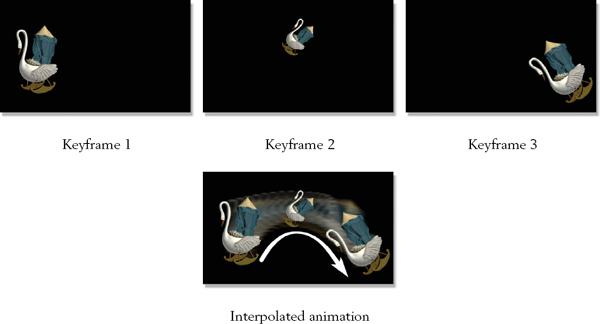
Figure 8-21 Multiple keyframes for move, scale, and rotate
Of course, the example in Figure 8-20 represented the simplest possible case of keyframe animation. Figure 8-21 illustrates a more realistic situation. This example has three keyframes at frames 1, 10, and 20, and instead of just a straight move it has a curved motion path, a scale, and a rotate. Note that at keyframe 2 the swan is much smaller and tilted over. This keyframe has a scale and a rotate to it in addition to a move. Keyframe 3 also has a scale and rotate as well as a position change compared with keyframe 2.
When the keyframes are entered the computer connects them together with splines, the mathematical “piano wire” that we met in Chapter 5, Creating a Mask. Of course, because the splines are being used to control animation we will now have to change their name from “splines” to “curves.” It’s another compositing rule. An example of these animation curves is shown in Figure 8-22, borrowed from Shake, the super compositing program from Apple. The computer uses splines to connect the keyframes with smooth, gently changing animation curves rather than simple straight lines. Simple straight lines of motion are both unnatural and boring so they are to be avoided at all costs.
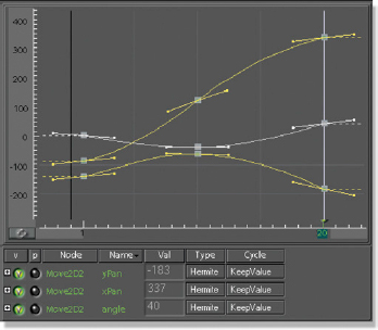
Figure 8-22 Animation curves
The fun part for the digital compositor is being promoted to digital animator and adjusting the splines to refine the shapes of the animation curves. Leaving the keyframes where they are, the slope of the splines can be adjusted to introduce fine variations in the animation such as an ease in or ease out, or changing the acceleration at just the right moment for an exhilarating motion accent. Whee.
8.6 MOTION BLUR
After carefully entering all your keyframes for an animation you may discover a disconcerting problem when you play it back at speed. The moving object may appear to stutter or chatter across the screen with a nasty case of motion strobing. The faster things move, the more motion strobing. What is happening is that the finished animation lacks motion blur, the natural smearing that an image gets when fast movement is captured by a film or video camera. Even CGI software adds motion blur for all moving objects.

Figure 8-23 Motion blur on fast moving objects
Figure 8-23 shows a few frames of a flying dove. The rapidly moving wings are motion blurred (smeared) across the film frame. Without this smearing in the direction of motion the bird’s wings would be in sharp focus and appear to pop from place to place on each frame—motion strobing.
Most modern digital compositing programs have a motion blur feature that works with their transforms to combat motion strobing. It is now well understood that you cannot go flying things around the screen without it. But what if your compositing program isn’t modern? A production expedient (a cheat) that you can try is to apply a one-directional blur in the direction of motion. It is not as realistic as a true motion blur, hard to animate if the target is moving irregularly, and it is difficult to find the right settings. But it is a sight better than motion strobing.
8.7 MOTION TRACKING
One of the truly wondrous things that a computer can do with moving pictures is motion tracking. The computer is pointed to a spot in the picture and then released to track that spot frame after frame for the length of the shot. This produces tracking data that can then be used to lock another image onto that same spot and move with it. The ability to do motion tracking is endlessly useful in digital compositing and you can be assured of getting to use it often. Motion tracking can be used to track a translation (move), a rotate, a scale, or any combination of the three. It can even track four points to be used with a corner pin. As it turns out, there are three different motion tracking technologies—a point tracker, a planar tracker, and a camera tracker. In this section we will be looking at the point tracker first, which is the most pervasive type.
One frequent application of motion tracking is to track a mask over a moving target. Say you have created a mask for a target object that itself does not move, but there is a camera move. You can draw the mask around the target on frame 1, and then motion track the shot to keep the mask following the target throughout the camera move. This is much faster and higher quality than rotoscoping the thing. Wire and rig removal is another very big use for motion tracking. A clean piece of the background can be motion tracked to cover up wires or a rig. Another important application is monitor screen replacement, where the four corners of the screen are motion tracked and then that data is given to a corner pin transform (Figure 8-8) to lock it onto a moving monitor face.
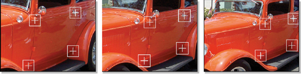
Figure 8-24 Four tracking points for a corner pin
We can see how motion tracking works with a point tracker using the corner pinning example in Figure 8-24, which shows three frames of a camera move on a parked car. The white cross-hairs are the tracking markers that lock onto the tracking points, the four points in the image that the computer locks onto to collect the motion tracking data. The tracking points are carefully chosen to be easy for the computer to lock onto. After the data is collected from the tracking points for the length of the shot it will be connected to the four control points of a corner pin operation so that it moves with the car.
At the start of the tracking process the operator positions the tracking markers over the tracking points, and then the computer makes a copy of the pixels outlined by each tracking marker. On the next frame the computer scans the image looking for groups of pixels that match the tracking points from the first frame. Finding the best match, it moves the tracking markers to the new location and then moves on to the next frame. Incredibly, it is able to find the closest fit to within a small fraction of a pixel.
The computer builds a frame-by-frame list of how much each tracking point has moved from its initial position in the first frame. This data is then used by a subsequent transform operation to move a second image in lock step with the original. Figure 8-25 shows the fruits of our motion tracking labor. Those really cool flames have been motion tracked to the side of the car door with a corner pin.

Figure 8-25 Cool flames tracked to hot rod with a corner pin
While this all sounds good, things frequently go wrong. By frequently, I mean most of the time. The example here was carefully chosen to provide a happy tracking story. In a real shot you may not have good tracking points. They may leave the frame halfway through the shot. Someone might walk in front of them. They might change their angle to the camera so much that the computer gets lost. The lens may distort the image so that the tracking data you get is all bent and wonky. The film might be grainy causing the tracking data to jitter. This is not meant to discourage you, but to brace you for realistic expectations and suggest things to look out for when setting up your own motion tracking.
8.8 STABILIZING A SHOT
Another great and important thing that can be done with motion tracking data is to stabilize a shot. But there is a downside that you should know about. Figure 8-26 shows a sequence of four frames with a “tequila” camera move (wobbly). The first step in the process is to motion track the shot, indicated by the white tracking marker locked onto the palm tree in each frame. Note how the tracking marker is moving from frame to frame along with the palm tree.
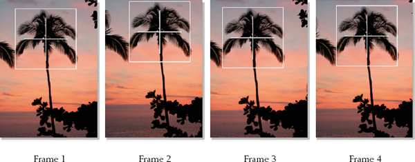
Figure 8-26 Original frames with camera movement
The motion tracking data collected from Figure 8-26 is now fed to a translation transform (OK, a move operation), but this time, instead of tracking something onto the moving target the data is inverted to pull the movement out of each frame. For example, if the motion tracking data for frame 3 shifted to the right by 10 pixels, then to stabilize it we would shift that frame to the left by 10 pixels to cancel out the motion. The tree is now rock steady in frame. Slick. However, shifting the picture left and right and up and down on each frame to recenter the palm tree has introduced unpleasant black edges to some of the frames in Figure 8-27. This is the downside I mentioned above that you should know about.
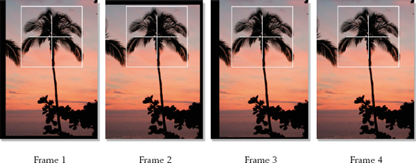
Figure 8-27 Stabilizing introduced black edges
We now have a stabilized shot with black edges that wander in and out of frame. Now what? The fix for this is to zoom in on the whole shot just enough to push all the black edges out of every frame. This needs to be done with great care, since this zoom operation also softens the image.
The first requirement is to find the correct center for the zoom. If the center of zoom is simply left at the center of the frame it will push the black edges out equally all around. The odds are, however, that you will have more black edges on one side than another, so shifting the center of zoom to the optimal location will permit you to push out the black edges with the least amount of zoom. The second requirement is to find the smallest possible zoom factor. The more you zoom into the shot, the softer it will be. Unfortunately, some softening is unavoidable. Better warn the client.
Just one more thing. If the camera is bouncing a lot it will introduce motion blur into the shot. After the shot is stabilized the motion blur will still be scattered randomly throughout the shot and may look weird. There is no practical fix for this. Better warn the client about this too.
(To see a movie showing camera motion blur in a stabilized shot download www.compositingVFX.com/CH08/Figure 8-27.mov.)
The previous sections on stabilizing a shot and match move were done using a point tracker. In this section we will see a completely different type of tracker that does a similar job, the planar tracker.
8.9.1 How Planar Tracking Works
A planar tracker takes advantage of the fact that there are flat planes all around us in the man-made world of floors, walls and streets, and even in the natural world of desert, lake and sky. Figure 8-28 shows just a few of the flat planes found in the man-made world that the planar tracker can use for its tracking calculations.
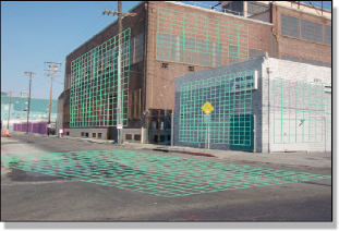
Figure 8-28 Flat planes used for planar tracking
First, a plane is masked off to identify it to the planar tracker. Then it compares the texture of the entire plane surface frame by frame to track its movement in the frame. It utilizes the fact that the texture is a flat plane to optimize the tracking calculations to match the texture for translate, rotate, scale, skew, and perspective. Because a planar tracker is looking at a much larger image area than a point tracker it is much less susceptible to noise (grain), dark images, changing lighting, obstructions, motion blur, and objects leaving frame.
The point tracker described in Section 8.7 made a copy of the pixels outlined by the tracking markers and held it to be used as a reference to match for all subsequent frames. In other words, it took a “snapshot” of a small piece of the image at frame 1 which it then compared to frame 2, then it compared frame 1 to frame 3, then frame 1 to frame 4, and so on. Of course, after several frames the reference taken on frame 1 may not match so well, so there are options to make a new reference if the tracker gets lost. It also means that if there are any significant differences between any later frame and frame 1, such as grain, changing lighting, motion blur, or obstructions, the tracker can “break lock” and fail.
But the planar tracker works entirely differently. First of all, it grabs a large block of pixels, not just the little rectangle of the point tracker. Second, the planar tracker compares frame 1 to frame 2, but grabs a new reference on frame 2 to compare it to frame 3, then another new reference to compare frame 3 to frame 4, and so on. By grabbing a new reference every frame and comparing it to an adjacent frame it is much less vulnerable to the variations that can flummox the point tracker. The large area used for the comparison also minimizes any tracking errors. However, because a new reference is created every frame a small amount of drift can be introduced into the tracking data because of accumulating errors, so there is a provision to remove any drift in the tracking data.
An immensely powerful feature of planar trackers is that if the tracking target is obscured or leaves frame, tracking data can still be generated if there is another coplanar surface in the picture. For example, referring back to Figure 8-28, if a truck were parked in front of the gray building on the right, the brown building on the left could be tracked instead because the two building faces are on the same plane. The tracking data only needs a single simple offset to reposition it over to the gray building.
8.9.2 What Planar Tracking is Used for
Like a point tracker, the tracking data generated by the planar tracker can be used in a wide variety of ways. Keep in mind that the planar tracker does not know or care whether the tracked object or the camera was moving, or both. It is capturing tracking data relative to the camera in all cases. In Figure 8-28 the camera would obviously be moving as buildings are normally static. In another case you might have a locked-off camera with the target moving through the frame. Or, you might have a moving camera on a moving object. Here are some of the very useful applications for the tracking data.
8.9.2.1 Motion Tracking
As we saw in Section 8.7 with the point tracker, motion tracking can be used to move one object to lock onto another object and move with it. Tracking data generates transformations, which is a description of the movement of an object in the image made up of translation (vertical and horizontal movement), rotation, scale, skew, and perspective. These transformations can be used to animate a graphic object, like a logo, to appear to stay locked to a moving object in the frame.

Figure 8-29 An example of planar motion tracking
Figure 8-29 illustrates the process of using planar motion tracking to “attach” a graphic object to a moving target. First, the live action bus is tracked with the planar tracker and the validity of the track is confirmed using the tracking grid. When the clip is played with the tracking grid turned on the grid appears to be “glued” to the side of the bus and moving with it without drifting. Once the tracking is confirmed the tracking grid is replaced by the graphic element so that it now appears to be attached to the side of the bus.
(To see a movie showing planar tracking on a moving train download www.compositingVFX.com/CH08/Figure 8-29.mov)
While motion tracking was illustrated here with a graphic element for simplicity, it is used for much more than this in visual effects shots. When doing wire removal or rig removal, bits and pieces of the unobstructed background must be motion tracked in to cover up the wires and rigs. In addition to making things disappear, motion tracking is also used to add things to a shot. One example would be to composite a bluescreen character over a moving background using motion tracking to lock him to the moving plate. The application of motion tracking in visual effects is virtually endless.
8.9.2.2 Corner Pinning
However, there are situations where just knowing the transformations to move one object with another is not enough. In some situations we also need to know where the corners of the source image need to be placed in the frame, such as with a monitor insert shot where we are replacing the contents of a monitor. This is what corner pinning is all about. The tracking data is converted into the location of each of the four corners of a moving video monitor, for example, and then the source image is “corner pinned” to the monitor’s corners frame by frame like the classic example in Figure 8-30. Of course, there are other uses for corner pinning such as tracking a picture into a picture frame or placing an outdoor scene through a window.
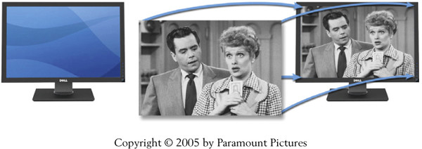
Figure 8-30 A “classic” example of four-corner pinning for a monitor insert shot
The transformation data generated by the planar tracker can also be used to stabilize a plate just as with a point tracker. While they do output exactly the same type of transformation data (translate, rotate, scale, etc.) the virtue of the planar tracker is its ability to lock onto more difficult targets. Of course, the problem of having to zoom into the stabilized plate to remove the black edges as we saw in Figure 8-27 remains the same.
8.9.2.4 Rotoscoping
Planar trackers are also a very useful tool to assist with rotoscoping. While there are a great many objects that are planar, in the real world there are many more that are not. Consider the human form, one of the most common rotoscoping targets. Surprisingly, the planar tracker will still get a good lock on a non-planar surface such as a face or hand, then this tracking data can be applied to the roto shape. What this gets you is a large part of the work being done for you by the machine. To be sure, the roto artists will have to step in and fine-tune the roto shape’s position and outline, but the tracking data from the planar tracker will have animated the roto spline to stay reasonably close to the target thus reducing the amount of work for the artist.
Figure 8-31 illustrates how the planar tracker can lock onto a moving target even if it is not a perfect plane. Of course, the less planar the tracking target is the less accurate the tracking data will be. However, the drift in the tracking data is not difficult to remove, and the corrected tracking data does much of the work of positioning and sizing the roto shape. Figure 8-32 shows the roto shape that has been tracked using the planar tracking data. With the machine doing much of the roto work it not only reduces the labor but also results in rotoscope mattes with less chatter and wobble.
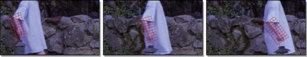
Figure 8-31 Planar tracking on a human target
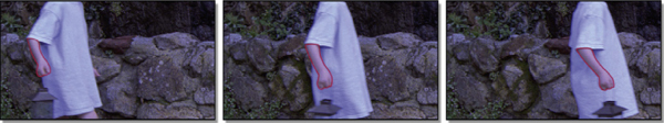
Figure 8-32 Planar tracking data applied to rotoscoping splines
8.10 MATCH MOVE
In the 3D compositing section of Chapter 3 (Section 3.8) camera tracking was covered in detail since it is a very large part of 3D compositing. However, camera tracking is also very important for creating animation for 2D compositing when doing a match move shot. A match move shot has a live action object that needs to be composited into a 3D environment with a matching camera move. The live action plate is camera tracked and that camera data is used to render a matching camera move on the 3D elements to create animation that lines up and moves with the live action element. In this workflow the CGI elements are rendered as images and then given to the compositor to composite as a 2D project.
As we saw in the camera tracking section of Chapter 3, in the process of a match move the computer is actually constructing a low-detail 3D model of the terrain it sees and figuring out where the camera is in 3D space along with what lens it is using. This 3D information is used to place CGI objects in their proper locations so they will be rendered with a camera move that matches the live action. Match move is such an important effect that good-sized visual effects facilities have a separate match move department and there are several dedicated and expensive match move programs available for purchase.
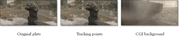
Figure 8-33 The elements of a match move shot
Figure 8-33 shows the elements of a typical match move shot. The original plate on the left is the live action with a sweeping camera move that orbits around the soldier. The middle frame shows the tracking points that the match move program selected to track the shot. They are marked with a white “X” to show the operator each tracking point it has locked onto. The CGI background is the element that must be properly positioned and rendered with a CGI camera move that matches the live action camera.
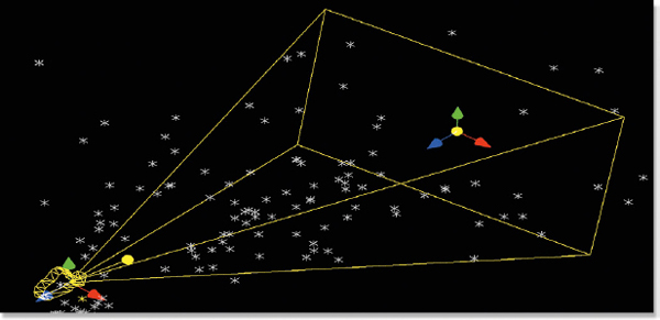
Figure 8-34 Point cloud with match move camera
The match move program plows through all of the frames of a shot locking onto as many tracking points as it can, typically dozens or even hundreds. The terrain is represented by the point cloud, which is the total of all of the tracking points the match move program could find. The example in Figure 8-34 shows how the point cloud extends far outside the camera’s field of view because it covers all of the terrain seen by the camera over the entire length of the shot.

Figure 8-35 Match moved CGI layers
The point cloud is then used by the CGI artists as a lineup reference to accurately position the 3D objects into the scene so that they sit in their proper locations relative to the live action. Figure 8-35 shows two layers of the CGI that used the point cloud as the lineup reference. The match move 3D camera data is then used to move the CGI camera through the CGI elements so they are rendered with the same camera move as the live action. In the example in Figure 8-35 the moving smoke and background layers were pre-composited into a single layer in preparation to receive the live action foreground.
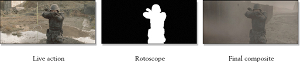
Figure 8-36 Live action layer rotoscoped and composited
The live action goes through a different sequence of operations before compositing. The main problem is that the live action character needs a matte for the composite but was not shot on bluescreen, so it has to be rotoscoped. Figure 8-36 shows the live action plate, its rotoscope, and the final composite of the live action over the CGI background from Figure 8-35. We now have all the elements necessary to produce the seamless action sequence shown in the six frames of Figure 8-37 plucked from the finished shot. Here the camera swoops almost 180 degrees around the soldier with the entire CGI environment moving in perfect sync.
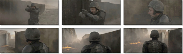
Figure 8-37 Finished match move action sequence
This particular example showed the match move done on a live action character in order to place him in an all-CGI world. This same technique can be used to place a CGI character into a live action world, such as adding CGI dinosaurs to a shot. To show a dinosaur running through the jungle the live action plate is first filmed by running through the jungle with the film camera. The jungle plate then goes to the match move department to be tracked and derive the terrain point cloud and camera move. The point cloud information is then used to position the CGI dinosaur onto the terrain and the camera move information is used to animate the CGI camera in sync with the live action camera. The dinosaur is then rendered and composited into the live action plate.
Since the dinosaur is a CGI element it comes with a fine matte. However, the dinosaur will need to be composited into the jungle, not over it. This means it will have to pass behind some leaves and foliage. To do that, a roto will be needed for every leaf and bush that passes in front of it.
(To see a shot breakdown movie of this match move download www.compositingVFX.com/CH08/match_move_vfx_breakdowns.mov)
8.11 THE WONDER OF WARPS
The transforms that we saw at the beginning of the chapter all had one thing in common, and that is that they moved or deformed an image uniformly over the entire frame. The corner pin, for example, allows you to pull on the four corners individually but the entire image is deformed as a whole—a global deformation, if you will.
Warps are different. The idea behind warps is to deform images differently in different parts of the picture—what are called local deformations. Warps even allow just one area to be deformed without altering any other part of the picture. Instead of having an image attached to a sheet of rubber that limits you to pulling on the four corners, warps can be thought of as applying the image to a piece of clay which allows you to deform any area you wish in any direction and to any degree. Much more fun.
We now take a look at three broad classes of warps—the mesh warp, the spline warp, and procedural warps. How each type of warp works will be explained, and then examples are given of how they are typically used in visual effects shots.
8.11.1 Mesh Warps
The mesh warp was the first generation image warper and still has many uses today. A simplified version of it makes up Photoshop’s current warp tool in the Edit > Transform > Warp menu. The basic idea is to create a grid or “mesh” of splines, attach it to an image, then, as you deform the mesh, the image deforms with it. Figure 8-38 shows the original graphic image and Figure 8-39 shows the overlaid mesh. The mesh is deformed in Figure 8-40 with the resulting deformed image in Figure 8-41. The mesh can also be animated, so a mesh warp animation of a waving flag could be made.

Figure 8-38 Original image

Figure 8-39 Overlaid mesh
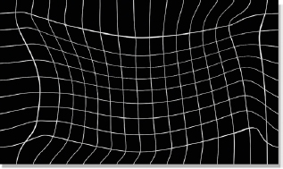
Figure 8-40 Deformed mesh

Figure 8-41 Deformed image
Because the mesh warp has a predefined grid of splines you cannot put control points anywhere you want. As a result, the mesh warp does not permit getting in close with fine warping detail. This means that it is best suited for broad overall warping of images such as the flag-waving example here. In a visual effects shot the main use for the mesh warp would be to gently reshape an element that was not exactly the right shape for the composite, such as fitting a new head on top of a body. If you are not careful, the mesh warp can introduce a lot of stretching in an image, which will in turn introduce softening.
8.11.2 Spline Warps
The spline warp is the second generation of warp tool. It was designed specifically to overcome the shortcomings of the mesh warp, namely the lack of detailed control, and is based on an entirely different concept. A spline is drawn around an area of interest in an image like the example in Figure 8-43 where warp splines have been added around the duck’s bill and feet. Then, as the splines are deformed the image is deformed. Splines can be placed anywhere in the image and they can deform only and exactly the part of the image you want by exactly how much you want. The original image in Figure 8-42 was spline warped to create the hysterical exaggeration in Figure 8-44.

Figure 8-42 Original image
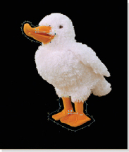
Figure 8-43 Warp splines added
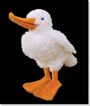
Figure 8-44 Hysterical exaggeration
While the spline warp is more powerful than the mesh warp it is also more complicated to work with. If a simple overall warp is needed the mesh warp is still the tool of choice. The spline warp comes into its own when you want to warp just specific regions of the image such as the duck’s bill and feet in Figure 8-43. Deforming just those regions would not be possible using a mesh warper. As we will see shortly, the spline warp is also used for a morph. Of course, the spline warp can also be animated not only to animate the shape change of the target object over time but also to follow the target object around from frame to frame like a roto.
8.11.3 Procedural Warps
Another entire class of image warps is the procedural warps, which just means to warp an image with a mathematical equation rather than by manually pulling on control points. The upside is that they are easy to work with because all you have to do is adjust the warp settings to get the look you want. The downside is their limited control in that the only warps you can do are those that the equation permits. You cannot customize the effect, but you can animate the warp settings so that the procedural warp changes over time.

Figure 8-45 Procedural warp examples
A few examples of procedural warps are shown in Figure 8-45. The pincushion warp is a common distortion introduced by camera lenses. In fact, there are specific lens warps with many more elaborate adjustments beyond pincushioning that are designed to accurately recreate lens distortions for visual effects shots. A swirl warp is shown in the next example and might be used as an effect in a television commercial. The turbulence warp could be animated to introduce heat waves in a shot or the distortions created by viewing something underwater.
8.12 THE MAGIC OF MORPHS
The morph provides the truly magical ability to seamlessly change one image into another right before the viewers’ eyes. This has been a dream of moviemakers ever since Lon Chaney Jr. appeared in his first Werewolf movie. Of course, this wondrous effect was immediately overused and run into the ground by every ad agency and B movie producer to the point that I actually saw a sign once in a visual effects studio that read, “friends don’t let friends morph.” Here we will see “the making of” the morph shown in Chapter 1 which has been re-released here as Figure 8-46.
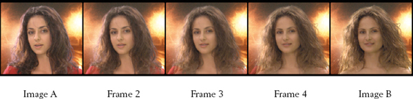
Figure 8-46 Morph animation sequence
It takes the computer two warps and a dissolve to make a morph, plus a talented digital artist to orchestrate it all, of course. The morph has an “A” side layer that dissolves (fades) into the “B” side layer. To morph image A into image B, we start by animating image A to warp into image B’s shape over the length of the shot like the example in Figure 8-47. Image A starts out with no warp (0%), then by the end of the shot is warped 100% to match the shape of image B. Note that while the model in Figure 8-47 is nice looking at the beginning, by the time she is 100% warped to image B she is not so nice looking anymore. For this reason we do the A to B dissolve in roughly the middle third of the shot so we never see an ugly 100% warped image.
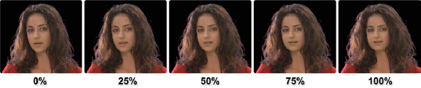
Figure 8-47 Image A warps from A to B
The warp animation for image B in Figure 8-48 starts the shot with a 100% warp to match the shape of image A, and then is “relaxed” over the length of the shot. Again, the not so attractive 100% warped image is never shown. If you compare the first frame of Figure 8-47 with the first frame of Figure 8-48 you will see that they have the same general outline, as do their last frames. As a result, the in-between frames also share the same general outline. We now have two synchronized “movies” of the warping faces and their mattes so all we have to do is dissolve between them and composite the results over an attractive background (Figure 8-46).
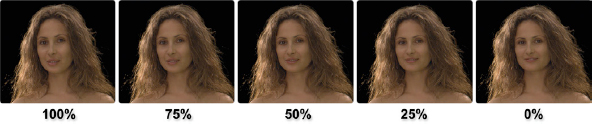
Figure 8-48 Image B relaxes from A to B
In any morph the A and B target objects must first be isolated from their backgrounds. Otherwise, the background stretches and pulls with the target and looks awful. Therefore the A and B images in the following example were both shot on bluescreen (or greenscreen) then keyed with a digital keyer prior to being warped. A side benefit of this is that their mattes also morph with them. If the target objects are not shot on a bluescreen then you get to roto them before doing the morph.
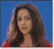
Figure 8-49 Image A
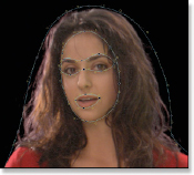
Figure 8-50 Warp splines
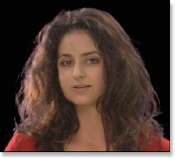
Figure 8-51 Image A warped to image B
The starting point for morphing image A (Figure 8-49) into image B (Figure 8-54) is first to move, scale, and rotate the images to pre-position them as close as possible. The less you have to push and pull on the ladies’ faces, the better they will look. Next is the placement of the warp splines on just those features that need a nudge in order to match their features to each other (Figure 8-50 and Figure 8-53). The general hair and face outlines needed a spline warp as did the mouth and eyes, but the noses were lined up close enough that they did not need to be warped and could “go natural.”

Figure 8-52 Image B warped to image A
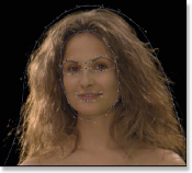
Figure 8-53 Warp splines
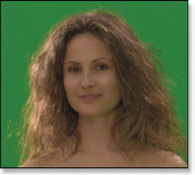
Figure 8-54 Image B