
13.1 INTRODUCTION
In the days of yore, there was video for TV and 35mm film for feature films. Period. Those days are gone forever. Video is still used for TV, but now it’s HD. And for feature films, there is still film, but now there is a long list of video and digital capture options that are being used in movie production today, and more coming every year. There is even a new term for this—the data-centric workflow—which encapsulates the all-digital workflow from digital capture to disk to post-production to projection. In this chapter we will sort out the various digital media and how they relate to visual effects compositing for feature films.
Photographing a feature film with a digital camera is now being referred to as “capture” instead of photographing or filming since there is no film involved. There are three classes of digital cameras that might be used to capture a movie and its visual effects elements:
• HD Video Cameras—some high-end HD video cameras such as the Sony CineAlta and Sony 950 can capture 4:4:4 video at 1920 × 1080 and have been used on some feature films. Some have log data options.
• Digital Cinema Cameras—these are very high-resolution cameras designed specifically for feature film work and the data-centric workflow using log data. Examples are the Panavision Genesis and the Thomson Viper.
• The RED—this, of course, is the premier digital cinema camera and stands to become the dominant camera for filmmaking. It is extremely high resolution with an outstanding dynamic range and uses standard 35mm film lenses.
From the low of The Blair Witch Project captured with a cheap handheld consumer video camera (later returned to Circuit City for a refund!!) to monstrous IMAX 70mm film cameras, the quality of the capture can vary hugely. And the quality of the captured image has a major impact on its suitability for visual effects. Too often inexperienced production crews use equipment that is not suitable or is even maladjusted for visual effects. The problem is that the captured images may look OK to the eye, but not to the computer. When a poorly captured clip is manipulated for visual effects it can disintegrate very quickly.
13.2 IMAGE SENSORS
Digital cameras have two basic technologies for capturing an image, typically referred to as “one-chip” and “three-chip” cameras. The one-chip camera has a single image sensor device commonly known as a Bayer array. The three-chip cameras have three separate CCD sensors and a prism to sort the red, green, and blue color light into them. In this section we will see how these devices work and the affect that they have on the final image for compositing.
13.2.1 Bayer Array
The basic idea of a Bayer array for the one-chip camera is that each light sensor in the array has a color filter over it so that it only sees one color—either red, green, or blue light. Further, the color filters are arranged in a pattern of four adjacent cells illustrated in Figure 13-1. Two of the cells have a green filter to collect green light, plus one cell for red and one for blue. The reason for this ratio is to roughly approximate human vision and the eye’s sensitivity to color. The eye’s perception of the brightness of a scene is made of a ratio of (approximately) 20% red, 70% green, and 10% blue light rays. The Bayer pattern roughly approximates this by collecting 25% red, 50% green, and 25% blue light. With some clever math manipulation the two green, one red, and one blue pixels are blended together to produce four separate pixels with unique RGB values.

Figure 13-1 Bayer pattern
To capture a color image the incoming light has to be “sorted” into red, green, and blue light, then have a sensor dedicated to each color. We will see another way of doing this sorting and sensing in the next section on CCD arrays. The downside to the Bayer arrangement is that the red sensor, for example, is discarding all the green and blue light that is falling on it so the Bayer array loses a lot of light. In fact, it will lose about two-thirds of the incoming light making it less sensitive in low-light situations. This is made up for by amplifying the data from the chip, but that in turn increases the amount of noise in the picture.
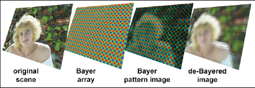
Figure 13-2 How a Bayer array digitizes an image
So let’s see how the Bayer array works to capture an image. Starting with the original scene in Figure 13-2, a lens focuses the image on the Bayer array just like it would on the film in a camera. The Bayer array converts the incoming light into digital signals representing the amount of red, green, and blue light landing on each cell. The result of this is the Bayer pattern image shown in Figure 13-2.
Now this does not look like a useful image, and indeed it is not. It is made up of adjacent red, green, and blue pixels instead of a nice RGB image. To convert the Bayer pattern into an RGB image it must be “de-Bayered,” that clever math manipulation mentioned above, which results in the de-Bayered image in Figure 13-2. You might also encounter the term “demosaicing” here since the Bayer pattern image is also called a mosaic by some.
Now we get to the part about compositing which pertains to the actual resolution of the de-Bayered image. Referring to Figure 13-2 again, let’s assume that the Bayer array depicted here was 2k resolution, so the resulting Bayer pattern image would also be 2k. Of course, only 50% of the pixels (1k worth) have green information, 25% have red information, and 25% blue information. We now do our clever math manipulation and output the de-Bayered image at 2k resolution. But is it really a 2k image? It will have 2k pixels, of course, but the information in those pixels is not 2k resolution. The RGB values have been interpolated from the red, green, and blue pixels of the Bayer pattern image.
So why are the one-chip image sensors so common? First of all, as mentioned above, a one-chip sensor is much more practical to build for high-resolution imaging—4k, 8k, and even higher. Second, the interpolation of the R, G, and B pixels into an RGB image works pretty darn well—but it is obviously not an honest 2k image. Third, they can be made physically large, say the size of a frame of 35mm film in a camera. This allows the use of existing 35mm film lenses which are frighteningly expensive, costing as much as the darn camera itself.
13.2.2 CCD Arrays
CCD arrays are the other image sensor technology used for high-end cameras which are often referred to as “three-chip” cameras because they have three CCD array chips as opposed to the one-chip for a Bayer array. The incoming white light (see Figure 13-3) is passed through a prism that sorts the light into red, green, and blue colors which then go to their individual CCD light sensors. There are no filters that block light so they use all of the available light and are therefore much more sensitive than Bayer arrays, giving them superior low-light performance.
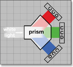
Figure 13-3 CCD array camera setup
Since the three-chip array captures an entire red, green, and blue image for every pixel, they are simply combined to output the full RGB image. No losses, no tricks, no clever math manipulation. But compared with one-chip sensors the three-chip sensors are larger, heavier, and more expensive. They cost more because there are three chips plus the added cost of the prism, a precision optical device. And precision optical devices do not obey Moore’s law.1
This affects compositing in a good way. Images captured with three-chip cameras have the most accurate color information, not interpolated and inferred color information like with the Bayer array. Further, these cameras can have 4:4:4 outputs which retain all of the color information and do not sub-sample it like a 4:2:2 video system. Because our greenscreen and bluescreen keyers use this color information to create the key, any reduction in the color information degrades the key. The greater low-light sensitivity also means less noise in the picture, which is always good for nice edges when keying.
13.3 HDR IMAGES
Digital capture for feature film visual effects is all about High Dynamic Range (HDR) images. The thing that separates the digital cinema cameras from video cameras is this much greater dynamic range. Not quite as good as film yet, but getting there. Some camera manufacturers claim dynamic ranges that meet or exceed film, but upon close inspection they are only valid for carefully restricted scenarios. So what is an HDR image and how does it affect compositing?
13.3.1 LDR vs. HDR Images
The universe of image capture devices can be sorted into two groups—low dynamic range (LDR) and high dynamic range (HDR). The LDR capture devices (video cameras and digital cameras) can only capture a limited range of scene luminance that is typically represented as between 0 and 1.0. When objects in the scene exceed the maximum sensitivity of the capture device (i.e., lights, fire, the sun) the resulting image is clipped at 1.0. The HDR capture devices (film and digital cinema cameras) can capture a much greater range of luminance, often 10 times more than the LDR devices. They still clip when their maximum range is exceeded, but they can deliver code values far above 1.0.
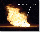
Figure 13-4 Original HDR scene
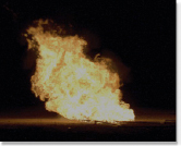
Figure 13-5 Image from an LDR capture device
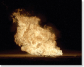
Figure 13-6 Image from an HDR capture device
We are using the term “luminance” here which is often confused with “brightness.” They are not at all the same. Luminance is a measure of the physical world—that is, how much light is reflecting from an object. Brightness is a human perception—how much brighter that object appears to the eye. To illustrate that they are very different things, if the luminance of an object (physical world) is doubled, the brightness (human perception) increases by only 18% due to the non-linear response of the eye.
Figure 13-4 shows a scene with a very high dynamic range of luminance. The hottest part of the fire contains code values as high as RGB 4.2 3.7 1.9. If this scene is captured by an LDR device such as a video camera or a digital camera the fire would be clipped at RGB 1.0 1.0 1.0 thus losing all the detail in the bright parts of the image. If this clipped image is then darkened down like Figure 13-5 the clipped parts of the fire appear as a flat slab of uniform gray. All of the bright detail is gone. If the same scene is captured with an HDR device such as film or a digital cinema camera, then darkened down by the same amount, the results would look like Figure 13-6. The image data is not clipped so all of the bright detail is retained. This is the entire reason for HDR capture devices. (To view a high resolution version see www.compositingVFX.com/CH13/Figure 13-06.exr)
Keep in mind that this clipping can occur in two different places—within the capture device, or later when the images are processed for compositing. The compositor is required to retain the full dynamic range of the HDR images upon output. The only exception would be with an LDR project such as HD video where some of the input clips were film scans which are HDR images. The film scans will have to be reduced to the limited HD video color space.
13.3.2 HDR Images on LDR Displays
One of the vexing problems doing feature film visual effects is that we are working with HDR images on an LDR display—the typical workstation flat panel monitor. This problem takes us back to Figure 13-4, which is what an HDR image would look like on a workstation monitor. The display of the image would be clipped like this, but the original image data would not. This means that if the RGB values of the original image were scaled down by lowering the brightness, the HDR image would still retain the bright detail like Figure 13-6. However, simply lowering the brightness does not produce the best appearance of an HDR image on an LDR display.
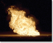
Figure 13-7 Tone mapped HDR image
This problem can be overcome by applying tone-mapping to the HDR image to artfully “squeeze” it into the limited dynamic range of the monitor display like the example in Figure 13-7. This is not a simple brightness change. The tone map redistributes the wide range of luminance values into the limited range of the monitor in a way that attempts to retain the original appearance of the image. This avoids clipping in the display and allows the digital artist to see the bright details of any composited effects, such as adding more fire to an explosion. It is essential that this tone-mapped version be in the viewer only and not affect the original image data.
13.3.3 HDR Cinema Clips
HDR cinema clips are high dynamic range clips captured with a digital cinema camera or 35mm film that has been digitized on a film scanner. The HDR clips are typically delivered as a 10-bit log Cineon or DPX files, which is covered in Section 13.4 Log Images.
The exposure range for HDR cinema clips is up to about 10 stops, depending on the capture device. A stop is a doubling of the scene illumination, so the maximum range of luminance it could capture would be 210:1, which is 1024:1. This means that the brightest object could be 1000 times brighter than the darkest object, allowing it to retain detail in specular highlights, light sources, fire, explosions, etc. Compare this with a standard video camera with a dynamic range of about 5½ stops. This means the maximum contrast ratio video can capture without clipping is a factor of less than 60:1. Film can do almost 1000:1, so film is definitely an HDR medium and video is definitely LDR. The digital cinema cameras are HDR devices too, some approaching film under carefully controlled circumstances.
Another source of HDR clips is CGI renders. Without the limitations of a capture device CGI can have code values far in excess of 1.0. Rather than being in a log format the HDR clips will typically be in an EXR file as a floating-point linear image. Of course, they will have the same display issues with the workstation monitors as the HDR cinema clips.
13.3.4 HDR Still Pictures
HDR still pictures are taking on an increasingly important role in visual effects and that trend is certain to increase in the future. Here are some current common applications of HDR images in visual effects:
• Image-based lighting—HDR photos are made from a location then used as a light source to illuminate a CGI scene rather than adding synthetic 3D lights. This results in much more photo realistic renders than standard 3D lighting.
• Digital matte paintings—when used in feature films (unlike video) the paintings have to be HDR images because both film and digital cinema is HDR.
• Camera projection—a common technique used in 3D compositing projects an HDR image onto cards or other geometry to be rephotographed with a 3D camera and composited with film scans or CGI.
Digital SLR cameras have a limited dynamic range, so in order to make an HDR image the camera will be set up to take several pictures with the aperture adjusted between takes to capture a wide range of exposures. The over-exposed pictures have plenty of dark detail but the brights are blown out. The under-exposed pictures have great bright detail but the darks are crushed. These multiple exposures are then “stacked up” on top each other using special software to create a composite HDR image far beyond the capability of the original camera.
Note the use of the term “darks” instead of “shadow” and “brights” instead of “highlights.” The reason is that HDR images cover such a wide range that it is not necessarily true that the darkest part of the picture will be a shadow or the brightest part will be a highlight so this is a more generic description of scene brightness content.
13.3.4.1 Exposure
Exposure for a camera means letting in more or less light to expose the film or whatever light sensor is being used to capture the scene. The key to understanding an HDR image is that it contains ALL of the exposures in one image. When looking at the HDR image on a display device like a monitor the image data vastly exceeds what the monitor can display. To choose what range of the HDR image will be visible in the display we can change the exposure of the HDR image digitally by increasing or decreasing its brightness by scaling the RGB values up or down. Increase the exposure (increase brightness) and the dark detail becomes visible at the expense of the brights. Decrease the exposure and the bright detail becomes visible at the expense of the dark detail.
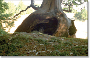
Figure 13-8 Exposure increased (courtesy ILM)
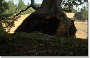
Figure 13-9 Exposure decreased
Figure 13-8 shows an HDR image shot into the shadows with broad daylight in the background. Normally this photograph wouldn’t even be printable, but because it is HDR it has retained all of the information in the darks and the lights. The exposure has been increased in this version to bring out the shadow detail but the bright daylight region in the background is completely blown out. Figure 13-9 shows what happens when the exposure is reduced. The shadows darken down but now the daylight area is perfectly exposed. The bottom line with an HDR image is that even though you can’t see it, the picture detail is retained in the original image.
13.3.4.2 EXR Images
The thing I love about EXR images is that they were in fact designed specifically for visual effects. Developed by ILM and released as freeware to the world, their main design goal was to hold a frame of digitized film in a linear data format that was lossless (no compression losses) with a reasonable file size. The feature that makes it ideal for CGI projects is its unlimited multichannel capability. With no compression the EXR file size is 50% larger than a comparable 10-bit Cineon/DPX file but there are some lossless compression options that actually make the file size smaller than Cineon.
Here are the three main features to know about the EXR file format:
• 16-bit float—each pixel is represented in a 16-bit floating-point format called “short float” because normal floating point uses 32 bits. This floating-point representation gives the EXR image incredible precision from the blackest black to the blazing brightness of the sun as it can encode up to 30 stops of exposure.
• Linear data—the image data is truly linear, meaning that any increase in the data values causes an equal increase in the luminance that it represents. This is in contrast to sRGB or Rec 709 color spaces that some will claim are linear, but are not. They are gamma corrected linear color spaces.
• Multi channel—like a Photoshop PSD file, an EXR file can have as many layers and channels as desired. They are user definable and can be expanded as needed.
13.3.4.3 Light Probes
One of the very important applications of HDR images is in the use of light probes to shoot HDR images used for image-based lighting for photo realistic CGI renders. A light probe is simply a highly polished chrome ball placed on the set or on location then photographed with multiple exposures as described above to create an HDR image. However, this image is a spherical projection of the scene surrounding the chrome ball and has captured almost a complete 360 degree image of the surroundings. This image is then remapped in the CGI program to a virtual sphere surrounding the CGI scene and used to light it.
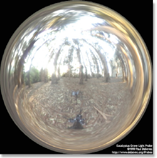
Figure 13-10 Exterior HDR light probe (courtesy Paul Debevec)
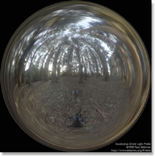
Figure 13-11 Reduced exposure shows detail in the brights
Figure 13-10 is a light probe of an exterior forest location. Based on the image shown here it looks like the sky is clipped and blown out. However, because this is an HDR image the reduced exposure version in Figure 13-11 reveals plenty of sky detail and even a setting sun on the left horizon. (To view a high resolution version see www.compositingVFX.com/CH13/Figure 13-10.hdr) Figure 13-12 is an interior light probe shot in Galileo’s tomb in Santa Croce Church, Florence, Italy. Again, the windows look over-exposed and blown out, but the reduced exposure version in Figure 13-13 shows plenty of light detail in the windows on the right. Both of these HDR images have code values in excess of 100!
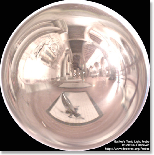
Figure 13-12 Interior HDR light probe (courtesy Paul Debevec)
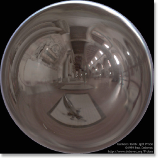
Figure 13-13 Reduced exposure shows detail in the brights
As we saw in Chapter 12, Working with Film, the modern workflow is to digitize the exposed film negative into a 10-bit log Cineon or DPX file format. However, digitized film is no longer the only source of log images. The film industry is moving towards digital cinema cameras which can output log image data that will be given directly to the VFX compositor to work with. To date there are four log formats you might encounter—Panalog, Redlog, Yedlog, and Viperlog—with more on the horizon. So what are these log images and how do we work with them?
13.4.1 The Virtue of Log
Log image data offers huge advantages over linear data such as from video cameras in two critical areas—plenty of detail in the darks (shadows) and vastly greater dynamic range. These are the big virtues of 35mm film, so the digital cinema cameras are attempting to emulate the capabilities of feature film. Film is log, so these cameras are also log, and for the same reason.
The basic concept is that the capture device (film camera or digital cinema camera) captures a much greater dynamic range image than the display device (film projector or digital cinema projector) can possibly show. This allows for great latitude to select the “sweet spot” from the original log image to compress and fit into the final display image for projection. With video what you capture is what you display. Not so with log images.
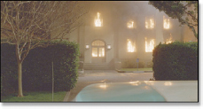
Figure 13-14 Original log image
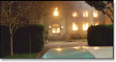
Figure 13-15 Normal exposure
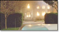
Figure 13-16 Over-exposed
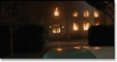
Figure 13-17 Under-exposed
Figure 13-14 shows the appearance of a typical log image. It is low contrast and appears all “blown out,” but in fact contains all the dark detail and dynamic range even though it doesn’t look like it. (To view a high resolution version see www.compositingVFX.com/CH13/Figure 13-14.tif) Figure 13-15 illustrates the results of producing a normal exposure as the display image (see Figure 13-15.tif). Figure 13-16 shows all the dark detail that is available in the bushes when the display image is over-exposed (see Figure 13-16.tif). In the normal exposure the bushes appeared to have no dark detail, but the over-exposed version shows that they indeed have plenty of detail. The most surprising is the under-exposed version in Figure 13-17 where all the detail in the flames can be seen (see Figure 13-17.tif). This illustrates the high dynamic range of information retained in the original log image. If this image had been captured by an HD video camera the flames would be clipped flat.
13.4.2 What is Log?
A 10-bit log image will have code values (data) that range from 0 to 1023, but not all code values are created equal. The relationship between the 10-bit code values and the scene illumination they represent is logarithmic. Figure 13-18 is a graph of the 10-bit log code values of a typical film scan plotted against the scene illumination, or how much light they represent. The low code values in the neighborhood of 95 (the tiny red sliver) represent the shadows or darks in the scene. Notice how steep the curve is in this region. This means that for very small increases in scene illumination there are a lot of code values. Alternately, you could say that there is a very small light difference between any two code values in this region.
The next zone, the midtones between, say, 250 and 685 (colored green), represents the normal exposure parts of the scene such as skin, clothes, and buildings. Again, the curve here is still steep so the code values do not represent a lot of scene illumination, but certainly more than in the darks. At last we get to the highlights from 685 and up (colored yellow). Here small changes in the code values represent very large changes in scene illumination.
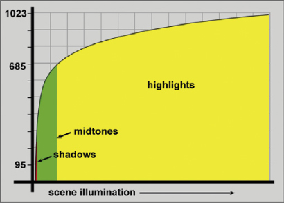
Figure 13-18 Log data curve
This may sound odd until you realize that the human eye is very sensitive to darks and shadows so small changes in light here are very noticeable. So with log images the code values in the darks represent very small changes in light so the eye cannot see the difference between two adjacent code values such as between 100 and 101. When we can see this difference it is called banding.
Conversely, the eye is very insensitive to changes in the brights. So in this region the code values represent very large changes in light. But again, the brightness change between two adjacent code values such as 900 and 901 is still imperceptible to the eye. The log encoding of a digital image is specifically designed to have lots of precision in the darks where we need it and far less in the brights where we don’t. The log curves for the digital cinema cameras have a somewhat different shape from film, but they all work on the same principle.
13.4.3 Working with Log Images
We have seen how 10-bit log data actually represents a varying amount of light between adjacent code values as they range from 0 to 1023. An image encoding system that represented the same amount of light between adjacent code values is called a linear system. That is the difference between linear and log.
The problem with log images is that while they are designed for efficiently compressing the picture data for storage and transfer, they are not good for compositing. For compositing, the log image must be converted to linear as soon as it is read from disk. To be honest, it is possible to work entirely in log space, but the rules are messy and it is very easy to get into trouble. As a result, virtually all compositing programs linearize log images, meaning that the image is converted from log to linear. Of course, when writing the finished composite back to disk it has to be converted back into log. The next step in the production pipeline, the Digital Intermediate and/or the film recorder, are both expecting 10-bit log images.
13.4.3.1 Converting Log to Linear
We can walk through the log to linear conversion process by referring to Figure 13-19 where the 10-bit log image (blue) is converted to linear floating point (gold). It turns out that log images are in fact high dynamic range images, so when converted to linear they produce code values well above 1.0. At the top end, log code value 1023 will become linear code value 11.5.
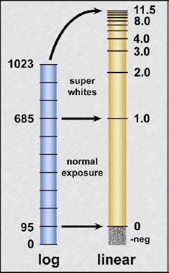
Figure 13-19 Log to linear conversion
Note that there are two “zones” identified in Figure 13-19, the normal exposure and the super whites. We want the normal exposure part of the log image to be “mapped” between linear code values 0 and 1.0, with the super whites (specular highlights, fire, explosions, the sun, etc.) mapped from code value 1.0 and up.
The log image is mapped into linear space by setting three parameters which can vary from film scan to film scan. The reason for this is that the original camera negative can be over- or underexposed (it invariably is) and this allows you to select the “sweet spot” in the log image to place into linear space between code values 0 and 1.0. The default values are black reference = 95 which will map across to linear code value 0, and white reference = 695 which maps over to 1.0. The third parameter is to adjust the display gamma for the best appearance. These values only apply to perfectly exposed film. Your log scans will vary, so these three parameters will invariably have to be tweaked.
13.4.3.2 Clipping
There is a danger when converting log images to linear, which is that some compositing programs will try to clip the linear data above 1.0 and below 0. This must not be allowed to happen. If the linear data above 1.0 is clipped then when the composite is converted back to log all of the code values above 685 will be gone, and along with them the super white parts of the picture.
One odd thing about converting log to linear is that it produces negative numbers. Referring to Figure 13-19 again, you can see how log code value 95 is mapped to linear code value 0. So what happens to, say, log code value 50? It must go below zero, hence a negative number. This is indicated in the illustration by the scratchy black patch labeled “-neg.” Log code value 95 is “black” as far as the image content is concerned, but the numbers below that contain the black grain. If the linear image is clipped at 0 when it is converted back to log there will be no code values below 95 and the black grain will be gone.
13.4.3.3 Converting Back to Log
OK, you have converted your log image to linear without any clipping, done your compositing in linear space, and now you are ready to render to disk to hand off your shot to the film recorder or the Digital Intermediate folks. As mentioned above, they are expecting a 10-bit log image just like the one you were given to do the VFX shot.
Here is the big rule for converting the composite from linear back to log: use exactly the same values that were used to convert it from log to linear originally. For example, if the log image was converted to linear using a black reference of 105, a white reference of 670, and a gamma of 1.8, then those exact values must be used to convert it back to log. If not, a major brightness and gamma change will occur in the new log image.
In fact, a standard check that should be done on any composited shot is to compare the original log image with the final rendered log composite. The background plate of the log composite should be identical to the original log image (plus anything you composited into the shot, of course). A swift check before starting a shot is to simply load in the log image, convert it to linear with the planned project settings, then convert it back to log and write it to disk. The two log images should be identical when compared. If the client has provided LUTs for this process then they should be used instead, but this in/out comparison test should always be done until the pipeline is known to be correct.
Again, all of these examples and values are for typical film log data. The digital cinema camera log data will have a somewhat different log curve, but the principles are the same.
1Moore’s law—declared by Gordon Moore, co-founder of Intel—stated in 1965 that every 18 months the number of resistors and transistors on a chip will double, making computers faster and cheaper.