Vector and matrix concepts have proved indispensable in the development of the subject of dynamics. The formulation of the equations of motion using the Newtonian or Lagrangian approach leads to a set of second-order simultaneous differential equations. For convenience, these equations are often expressed in vector and matrix forms. Vector and matrix identities can be utilized to provide much less cumbersome proofs of many of the kinematic and dynamic relationships. In this chapter, the mathematical tools required to understand the development presented in this book are discussed briefly. Matrices and matrix operations are discussed in the first two sections. Differentiation of vector functions and the important concept of linear independence are discussed in Section 3. In Section 4, important topics related to three-dimensional vectors are presented. These topics include the cross product, skew-symmetric matrix representations, Cartesian coordinate systems, and conditions of parallelism. The conditions of parallelism are used in this book to define the kinematic constraint equations of many joints in the three-dimensional analysis. Computer methods for solving algebraic systems of equations are presented in Sections 5 and 6. Among the topics discussed in these two sections are the Gaussian elimination, pivoting and scaling, triangular factorization, and Cholesky decomposition. The last two sections of this chapter deal with the QR decomposition and the singular value decomposition. These two types of decompositions have been used in computational dynamics to identify the independent degrees of freedom of multibody systems. The last two sections, however, can be omitted during a first reading of the book.
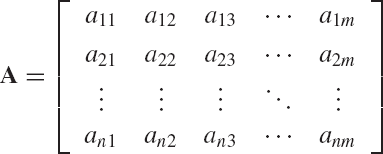
An m × n matrix A is an ordered rectangular array that has m × n elements. The matrix A can be written in the form
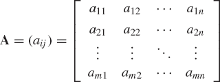
The matrix A is called an m × n matrix since it has m rows and n columns. The scalar element aij lies in the ith row and jth column of the matrix A. Therefore, the index i, which takes the values 1, 2, ..., m denotes the row number, while the index j, which takes the values 1, 2, ..., n denotes the column number.
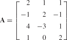
A matrix A is said to be square if m = n. An example of a square matrix is
In this example, m = n = 3, and A is a 3 × 3 matrix.
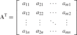
The transpose of an m × n matrix A is an n × m matrix denoted as AT and defined as
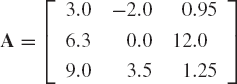
For example, let A be the matrix

The transpose of A is
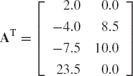
That is, the transpose of the matrix A is obtained by interchanging the rows and columns.
A square matrix A is said to be symmetric if aij = aji. The elements on the upper-right half of a symmetric matrix can be obtained by flipping the matrix about the diagonal. For example,

is a symmetric matrix. Note that if A is symmetric, then A is the same as its transpose; that is, A = AT.
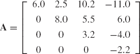
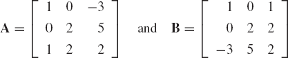
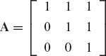
A square matrix is said to be an upper-triangular matrix if aij = 0 for i > j. That is, every element below each diagonal element of an upper-triangular matrix is zero. An example of an upper-triangular matrix is
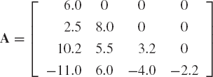
A square matrix is said to be a lower-triangular matrix if aij = 0 for j > i. That is, every element above the diagonal elements of a lower-triangular matrix is zero. An example of a lower-triangular matrix is
The diagonal matrix is a square matrix such that aij = 0 if i ≠ j, which implies that a diagonal matrix has element aii along the diagonal with all other elements equal to zero. For example,
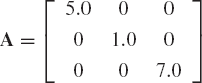
is a diagonal matrix.
The null matrix or zero matrix is defined to be a matrix in which all the elements are equal to zero. The unit matrix or identity matrix is a diagonal matrix whose diagonal elements are nonzero and equal to 1.
A skew-symmetric matrix is a matrix such that aij = −aji. Note that since aij = −aji for all i and j values, the diagonal elements should be equal to zero. An example of a skew-symmetric matrix
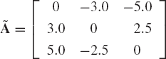
It is clear that for a skew-symmetric matrix,
The trace of a square matrix is the sum of its diagonal elements. The trace of an n × n identity matrix is n, while the trace of a skew-symmetric matrix is zero.
In this section we discuss some of the basic matrix operations that are used throughout the book.
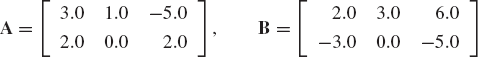
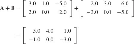
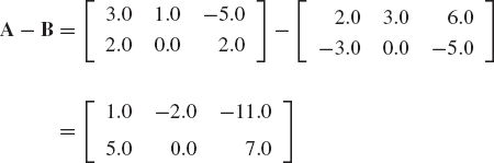
The sum of two matrices A and B, denoted by A + B, is given by
where bij are the elements of B. To add two matrices A and B, it is necessary that A and B have the same dimension; that is, the same number of rows and the same number of columns. It is clear from Eq. 3 that matrix addition is commutative, that is,
Matrix addition is also associative, because
The product of two matrices A and B is another matrix C, defined as
The element cij of the matrix C is defined by multiplying the elements of the ith row in A by the elements of the jth column in B according to the rule
Therefore, the number of columns in A must be equal to the number of rows in B. If A is an m × n matrix and B is an n × p matrix, then C is an m × p matrix. In general, AB ≠ BA. That is, matrix multiplication is not commutative. Matrix multiplication, however, is distributive; that is, if A and B are m × p matrices and C is a p × n matrix, then
Example 2.2
Let
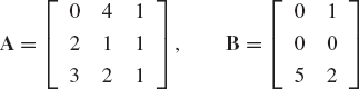
Then
The product BA is not defined in this example since the number of columns in B is not equal to the number of rows in A.
The associative law is valid for matrix multiplications. If A is an m × p matrix, B is a p × q matrix, and C is a q × n matrix, then
Matrix partitioning is a useful technique that is frequently used in manipulations with matrices. In this technique, a matrix is assumed to consist of submatrices or blocks that have smaller dimensions. A matrix is divided into blocks or parts by means of horizontal and vertical lines. For example, let A be a 4 × 4 matrix. The matrix A can be partitioned by using horizontal and vertical lines as follows:

In this example, the matrix A has been partitioned into four submatrices; therefore, we can write A compactly in terms of these four submatrices as
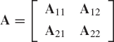
where
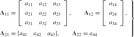
Apparently, there are many ways by which the matrix A can be partitioned. As we will see in this book, the way the matrices are partitioned depends on many factors, including the applications and the selection of coordinates.
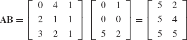
Partitioned matrices can be multiplied by treating the submatrices like the elements of the matrix. To demonstrate this, we consider another matrix B such that AB is defined. We also assume that B is partitioned as follows:
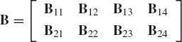
The product AB is then defined as follows:
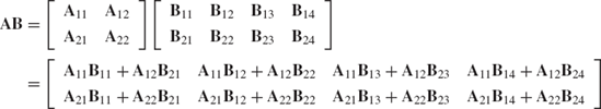
When two partitioned matrices are multiplied we must make sure that additions and products of the submatrices are defined. For example, A11B12 must have the same dimension as A12B22. Furthermore, the number of columns of the submatrix Aij must be equal to the number of rows in the matrix Bjk. It is, therefore, clear that when multiplying two partitioned matrices A and B, we must have for each vertical partitioning line in A a similarly placed horizontal partitioning line in B.
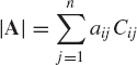
The determinant of an n × n square matrix A, denoted as |A|, is a scalar defined as

To be able to evaluate the unique value of the determinant of A, some basic definitions have to be introduced. The minor Mij corresponding to the element aij is the determinant formed by deleting the ith row and jth column from the original determinant |A|. The cofactor cij of the element aij is defined as
Using this definition, the value of the determinant in Eq. 15 can be obtained in terms of the cofactors of the elements of an arbitrary row i as follows:
Clearly, the cofactors cij are determinants of order n − 1. If A is a 2 × 2 matrix defined as

the cofactors cij associated with the elements of the first row are
According to the definition of Eq. 17, the determinant of the 2 × 2 matrix A using the cofactors of the elements of the first row is
If A is 3 × 3 matrix defined as
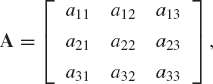
the determinant of A in terms of the cofactors of the first row is given by
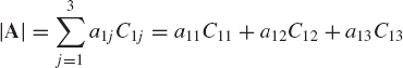
where

That is, the determinant of A is
One can show that the determinant of a matrix is equal to the determinant of its transpose, that is,
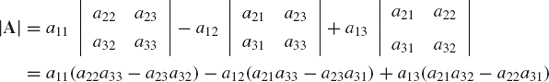
and the determinant of a diagonal matrix is equal to the product of the diagonal elements. Furthermore, the interchange of any two columns or rows only changes the sign of the determinant. If a matrix has two identical rows or two identical columns, the determinant of this matrix is equal to zero. This can be demonstrated by the example of Eq. 24. For instance, if the second and third rows are identical, a21 = a31, a22 = a32, and a23 = a33. Using these equalities in Eq. 24, one can show that the determinant of the matrix A is equal to zero. More generally, a square matrix in which one or more rows (columns) are linear combinations of other rows (columns) has a zero determinant. For example,
have zero determinants since in A the last row is the sum of the first two rows and in B the last column is the sum of the first two columns.
A matrix whose determinant is equal to zero is said to be a singular matrix. For an arbitrary square matrix, singular or nonsingular, it can be shown that the value of the determinant does not change if any row or column is added to or subtracted from another.
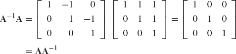
A square matrix A−1 that satisfies the relationship
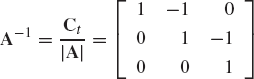
where I is the identity matrix, is called the inverse of the matrix A. The inverse of the matrix A is defined as
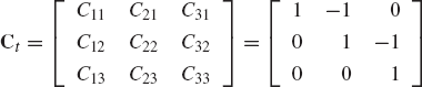
where Ct is the adjoint of the matrix A. The adjoint matrix Ct is the transpose of the matrix of the cofactors cij of the matrix A.
Example 2.3
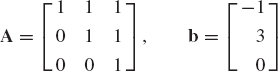
Determine the inverse of the matrix
Solution. The determinant of the matrix A is equal to 1, that is,
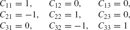
The cofactors of the elements of the matrix A are
The adjoint matrix, which is the transpose of the matrix of the cofactors, is given by
Therefore,
If A is the 2 × 2 matrix
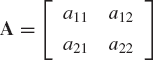
the inverse of A can be written simply as
where |A|=a11a22 − a12a21.
If the determinant of A is equal to zero, the inverse of A does not exist. This is the case of a singular matrix. It can be verified that
which implies that the transpose of the inverse of a matrix is equal to the inverse of its transpose.
If A and B are nonsingular square matrices, then
In general, the inverse of the product of square nonsingular matrices A1, A2, ..., An−1, An is
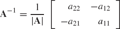
This equation can be used to define the inverse of matrices that arise naturally in mechanics. One of these matrices that appears in the formulations of the recursive equations of mechanical systems is

The matrix D can be written as the product of n − 1 matrices as follows:
from which
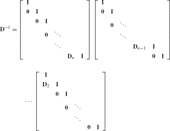
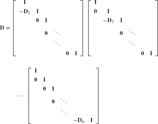
Therefore, the inverse of the matrix D can be written as
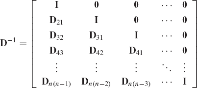
where
A square matrix A is said to be orthogonal if
In this case AT = A−1.
That is, the inverse of an orthogonal matrix is equal to its transpose. An example of orthogonal matrices is
where θ is an arbitrary angle,

and ν1, ν2, and ν3 are the components of an arbitrary unit vector v, that is, v = [ν1 ν2 ν3]T. While
It can be shown that
Using these identities, one can verify that the matrix A of Eq. 40 is an orthogonal matrix. In addition to the orthogonality, it can be shown that the matrix A and the unit vector v satisfy the following relationships:
In computational dynamics, the elements of a matrix can be implicit or explicit functions of time. At a given instant of time, the values of the elements of such a matrix determine whether or not a matrix is singular. For example, consider the following two matrices, which depend on the three variables ϕ, θ, ψ:
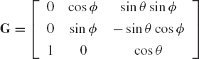
and
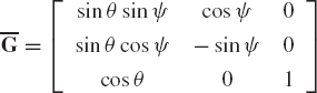
The inverses of these two matrices are given as

and
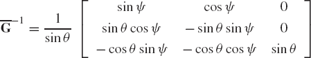
It is clear that these two inverses do not exist if sin θ = 0. The reader, however, can show that the matrix A, defined as
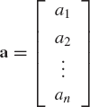
An n-dimensional vector a is an ordered set
of n scalars. The scalar ai, i = 1, 2, ..., n is called the ith component of a. An n-dimensional vector can be considered as an n × 1 matrix that consists of only one column. Therefore, the vector a can be written in the following column form:
The transpose of this column vector defines the n-dimensional row vector
The vector a of Eq. 50 can also be written as
By considering the vector as special case of a matrix with only one column or one row, the rules of matrix addition and multiplication apply also to vectors. For example, if a and b are two n-dimensional vectors defined as
then a + b is defined as
Two vectors a and b are equal if and only if ai = bi for i = 1, 2, ..., n.
The product of a vector a and scalar α is the vector
The dot, inner, or scalar product of two vectors a = [a1a2...an]T and b = [b1b2...bn]T is defined by the following scalar quantity:
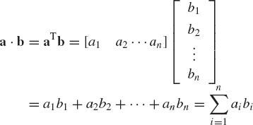
It follows that a · b = b · a.
Two vectors a and b are said to be orthogonal if their dot product is equal to zero, that is, a · b = aTb = 0. The length of a vector a denoted as |A| is defined as the square root of the dot product of a with itself, that is,
The terms modulus, magnitude, norm, and absolute value of a vector are also used to denote the length of a vector. A unit vector is defined to be a vector that has length equal to 1. If â is a unit vector, one must have
If a = [a1 a2 ... an]Ti s an arbitrary vector, a unit vector â collinear with the vector a is defined by
Example 2.4
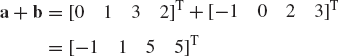
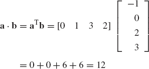
Let a and b be the two vectors
Then
The dot product of a and b is
Unit vectors along a and b are
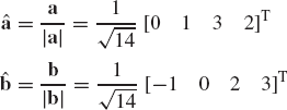
It can be easily verified that
In many applications in mechanics, scalar and vector functions that depend on one or more variables are encountered. An example of a scalar function that depends on the system velocities and possibly on the system coordinates is the kinetic energy. Examples of vector functions are the coordinates, velocities, and accelerations that depend on time. Let us first consider a scalar function f that depends on several variables q1, q2, ... , and qn and the parameter t, such that
where q1, q2, ..., qn are functions of t, that is, qi = qi(t).
The total derivative of f with respect to the parameter t is
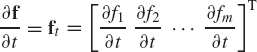
which can be written using vector notation as
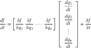
This equation can be written as
in which ∂f/∂t is the partial derivative of f with respect to t, and
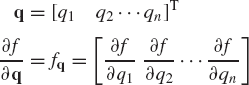
That is, the partial derivative of a scalar function with respect to a vector is a row vector. If f is not an explicit function of t, ∂f/∂t = 0.
Example 2.5
Consider the function
where q1 and q2 are functions of the parameter t. The total derivative of f with respect to the parameter t is
where
Hence
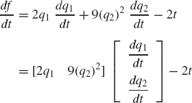
where ∂f/∂q can be recognized as the row vector
Consider the case of several functions that depend on several variables. These functions can be written as
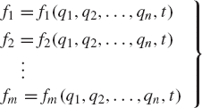
where qi = qi(t), i = 1, 2, ..., n. Using the procedure previously outlined in this section, the total derivative of an arbitrary function fj can be written as
in which ∂fj/∂q is the row vector
It follows that
where
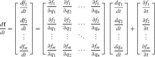
Equation 68 can also be written as
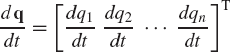
where the m × n matrix ∂f/∂q, the n-dimensional vector dq/dt, and the m-dimensional vector ∂f/∂t can be recognized as
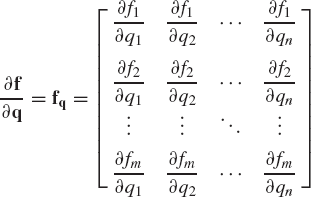
If the function fj is not an explicit function of the parameter t, then ∂fj/∂t is equal to zero. Note also that the partial derivative of an m-dimensional vector function f with respect to an n-dimensional vector q is the m × n matrix fq defined by Eq. 71.
Example 2.6
Consider the vector function f defined as
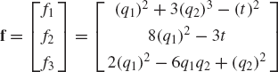
The total derivative of the vector function f is
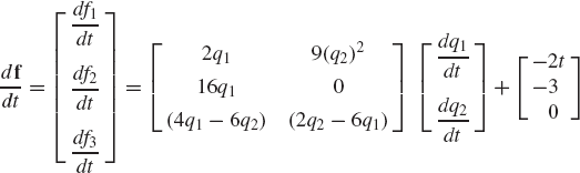
where the matrix fq can be recognized as
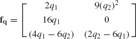
and the vector ft is
In the analysis of mechanical systems, we may also encounter scalar functions in the form
Following a similar procedure to the one outlined previously in this section, one can show that
If A is a symmetric matrix, that is A = AT, one has
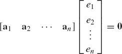
The vectors a1, a2, ..., an are said to be linearly dependent if there exist scalars e1, e2, ..., en, which are not all zeros, such that
Otherwise, the vectors a1, a2, ..., an are said to be linearly independent. Observe that in the case of linearly independent vectors, not one of these vectors can be expressed in terms of the others. On the other hand, if Eq. 77 holds, and not all the scalars e1, e2, ..., en are equal to zeros, one or more of the vectors a1, a2, ..., an can be expressed in terms of the other vectors.
Equation 77 can be written in a matrix form as
which can also be written as
If the vectors a1, a2, ..., an are linearly dependent, the system of homogeneous algebraic equations defined by Eq.79 has a nontrivial solution. On the other hand, if the vectors a1, a2, ..., an are linearly independent vectors, then A must be a nonsingular matrix since the system of homogeneous algebraic equations defined by Eq. 79 has only the trivial solution e = A−10 = 0. In the case where the vectors a1, a2, ..., an are linearly dependent, the square matrix A must be singular. The number of linearly independent columns in a matrix is called the column rank of the matrix. Similarly, the number of independent rows is called the row rank of the matrix. It can be shown that for any matrix, the row rank is equal to the column rank is equal to the rank of the matrix. Therefore, a square matrix that has a full rank is a matrix that has linearly independent rows and linearly independent columns. Thus, we conclude that a matrix that has a full rank is a nonsingular matrix.
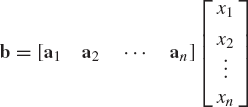
If a1, a2, ..., an are n-dimensional linearly independent vectors, any other n-dimensional vector can be expressed as a linear combination of these vectors. For instance, let b be another n-dimensional vector. We show that this vector has a unique representation in terms of the linearly independent vectors a1, a2, ..., an. To this end, we write b as
where x1, x2, ..., and xn are scalars. In order to show that x1, x2, ..., and xn are unique, Eq. 81 can be written as
which can be written as
where A is a square matrix defined by Eq. 80 and x is the vector
Since the vectors a1, a2, ..., an are assumed to be linearly independent, the coefficient matrix A in Eq. 83 has a full row rank, and thus it is nonsingular. This system of algebraic equations has a unique solution x, which can be written as x=A−1b. That is, an arbitrary n-dimensional vector b has a unique representation in terms of the linearly independent vectors a1, a2, ..., an.
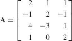
A familiar and important special case is the case of three-dimensional vectors. One can show that the three vectors

are linearly independent. Any other three-dimensional vector b = [b1 b2 b3]T can be written in terms of the linearly independent vectors a1, a2, and a3 as
where the coefficients x1, x2, and x3 can be recognized in this special case as
The coefficients x1, x2, and x3 are called the coordinates of the vector b in the basis defined by the vectors a1, a2, and a3.
Example 2.7
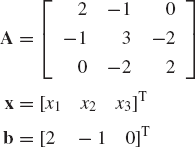
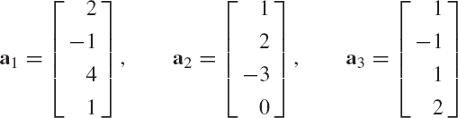
Show that the vectors

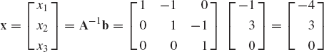
are linearly independent. Find also the representation of the vector b = [−1 3 0]T in terms of the vectors a1, a2, and a3.
Solution. In order to show that the vectors a1, a2, and a3 are linearly independent, we must show that the relationship
holds only when e1 = e2 = e3 = 0. To show this, we write
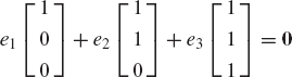
which leads to
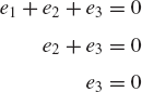
Back substitution shows that
which implies that the vectors a1, a2, and a3 are linearly independent.
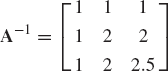
To find the unique representation of the vector b in terms of these linearly independent vectors, we write
which can be written in matrix form as
where
Hence, the coordinate vector x can be obtained as
A special case of n-dimensional vectors is the three-dimensional vector. Three-dimensional vectors are important in mechanics because the position, velocity, and acceleration of a particle or an arbitrary point on a rigid or deformable body can be described in space using three-dimensional vectors. Since these vectors are a special case of the more general n-dimensional vectors, the rules of vector additions, dot products, scalar multiplications, and differentiations of these vectors are the same as discussed in the preceding section.
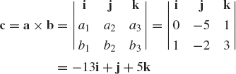
Consider the three-dimensional vectors a=[a1 a2 a3]T, and b = [b1 b2 b3]T. These vectors can be defined by their components in the three-dimensional space XYZ. Therefore, the vectors a and b can be written in terms of their components along the X, Y, and Z axes as
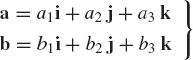
where i, j, and k are unit vectors defined along the X, Y, and Z axes, respectively.
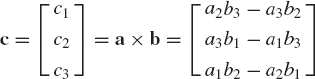
The cross or vector product of the vectors a and b is another vector c orthogonal to both a and b and is defined as
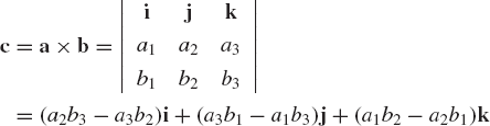
which can also be written as
This vector satisfies the following orthogonality relationships:
It can also be shown that
If a and b are parallel vectors, it can be shown that c = a × b = 0. It follows that a × a=0. If a and b are two orthogonal vectors, that is, aTb = 0, it can be shown that |c| = |a||b|. The following useful identities can also be verified:


The vector cross product as defined by Eq. 90 can be represented using matrix notation. By using Eq. 90, one can write a × b as
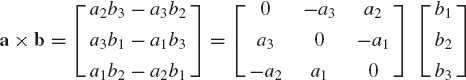
which can be written as
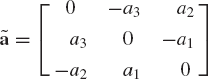
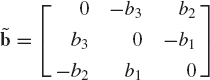
where ã is the skew-symmetric matrix associated with the vector a and defined as
Similarly, the cross product b × a can be written in a matrix form as
where
If â is a unit vector along the vector a, it is clear that â × a = −a × â = 0. It follows that -ãâ = ãT â = 0.
In some of the developments presented in this book, the constraints that represent mechanical joints in the system can be expressed using a set of algebraic equations. Quite often, one encounters a system of equations that can be written in the following form:
where a = [a1 a2 a3]T and x = [x1 x2 x3]T. Using the notation of the skew symmetric matrices, Eq. 99 can be written as
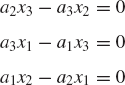
where ã is defined by Eq. 96. Equation 100 leads to the following three algebraic equations:
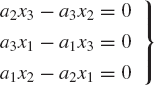
These three equations are not independent because, for instance, adding a1/a3 times the first equation to a2/a3 times the second equation leads to the third equation. That is, the system of equations given by Eq. 99, or equivalently Eq. 100, has at most two independent equations. This is due primarily to the fact that the skew-symmetric matrix ã of Eq. 96 is singular and its rank is at most two.
Example 2.9
Let a and b be the three-dimensional vectors
Determine the skew-symmetric matrices ã and
Solution. The skew-symmetric matrices ã and
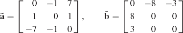
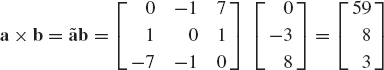
The cross product a × b can be written as
Example 2.10
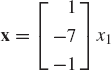
Solve the system of equations ãx = 0, where a is the vector a = [−1 7 1]T.
Solution. As pointed out in this section, the system of equations ãx = 0 has only two independent equations since the rank of the skew-symmetric matrix ã is at most two. Consequently, this system of equations has a nontrivial solution that can be determined to within an arbitrary constant. The equation ãx = 0 can be written explicitly as
Since this system has only two independent equations, we can determine x2 and x3 in terms of x1. This leads to
This solution satisfies the three algebraic equations, and for a given value of x1, the other two variables x2 and x3 can be determined. Using the components of the vector a, we have
Therefore, the solution vector x is
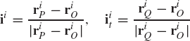
In spatial dynamics, several sets of orientation coordinates can be used to describe the three-dimensional rotations. Some of these orientation coordinates, as will be demonstrated in Chapter 7, lack any clear physical meaning, making it difficult in many applications to define the initial configuration of the bodies using these coordinates. One method which is used in computational dynamics to define a Cartesian coordinate system is to introduce three points on the rigid body and use the vector cross product to define the location and orientation of the body coordinate system in the three-dimensional space. To illustrate the procedure for using the vector cross product to achieve this goal, we consider body i which has a coordinate system XiYiZi with its origin at point Oi as shown in Fig. 2-1. Two other points Pi and Qi are defined such that point Pi lies on the Xi axis and point Qi lies in the XiYi plane. If the position vectors of the three points Oi, Pi, and Qi are known and defined in the XYZ coordinate system by the vectors riO, riP, and riQ, one can first define the unit vectors ii and iit as
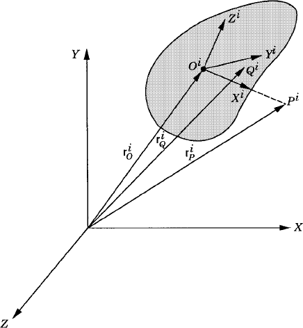
where ii defines a unit vector along the Xi axis. It is clear that a unit vector ki along the Zi axis is defined as
A unit vector along the Yi axis can then be defined as
The vector riO defines the position vector of the reference point Oi in the XYZ coordinate system, while the 3 × 3 matrix
as will be shown in Chapter 7, completely defines the orientation of the body coordinate system XiYiZi with respect to the coordinate system XYZ. This matrix is called the direction cosine transformation matrix.
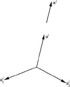
In formulating the kinematic constraint equations that describe a mechanical joint between two bodies in a multibody system, the cross product can be used to indicate the parallelism of two vectors on the two bodies. For instance, if ai and aj are two vectors defined on bodies i and j in a multibody system, the condition that these two vectors remain parallel is given by
As pointed out previously, this equation contains three scalar equations that are not independent. An alternative approach to formulate the parallelism condition of the two vectors ai and aj is to use two independent dot product equations. To demonstrate this, we form the orthogonal triad ai, ai1, and ai2, defined on body i as shown in Fig. 2-2. It is clear that if the vectors ai and aj are to remain parallel, one must have
These are two independent scalar equations that can be used instead of using the three dependent scalar equations of the cross product.
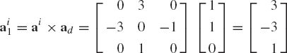
For a given nonzero vector ai, a simple computer procedure can be used to determine the vectors ai1 and ai2 such that ai, ai1, and ai2 form an orthogonal triad. In this procedure, we first define a nonzero vector ad that is not parallel to the vector ai. The vector ad can simply be defined as the three-dimensional vector that has one zero element and all other elements equal to one. The location of the zero element is chosen to be the same as the location of the element of ai that has the largest absolute value. The vector ai1 can then be defined as
Clearly, ai1 is perpendicular to ai. One can then define ai2 that completes the orthogonal triad ai, ai1, and ai2 as
To demonstrate this simple procedure, consider the vector ai defined as ai = [1 0 −3]T. The element of ai that has the largest absolute value is the third element. Therefore, the vector ad is defined as ad = [1 1 0]T. The vector ai1 is then defined as
and the vector ai2 is
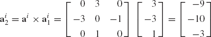
The method of finding the inverse can be utilized in solving a system of n algebraic equations in n unknowns. Consider the following system of equations:
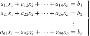
where aij, i, j = 1, 2, ..., n are known coefficients, b1, b2, ..., and bn are given constants, and x1, x2, ..., and xn are unknowns. The preceding system of equations can be written in a matrix form as
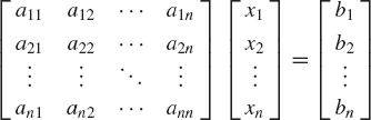
This system of algebraic equations can be written as
where the coefficient matrix A is
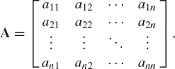
and the vectors x and b are given by
If the coefficient matrix A in Eq. 112 has a full rank, the inverse of this matrix does exist. Multiplying Eq. 112 by the inverse of A, one obtains
Since A−1A=I, where I is the identity matrix, the solution of the system of algebraic equations can be defined as
It is clear from this equation that if A is a nonsingular matrix, the homogeneous system of algebraic equations Ax = 0 has only the trivial solution x = 0.
Example 2.11
Find the solution of the system of algebraic equations
Solution. This system of algebraic equations can be written in a matrix form as
which can also be written as
where
It can be verified that the inverse of the matrix A is
Using this inverse, the solution of the system of equations can be written as
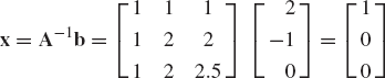
Since the matrix A is nonsingular, this solution is unique.
The method of finding the inverse is rarely used in practice to solve a system of algebraic equations. This is mainly because the explicit construction of the inverse of a matrix by using the adjoint matrix approach, which requires the evaluation of the determinant and the cofactors, is computationally expensive and often leads to numerical errors.
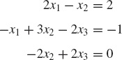
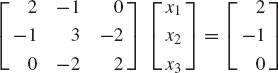
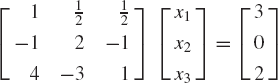
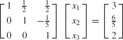
The Gaussian elimination method is an alternative approach for solving a system of algebraic equations. This approach, which is based on the idea of eliminating variables one at a time, requires a much smaller number of arithmetic operations as compared with the method of finding the inverse. The Gaussian elimination consists of two main steps: the forward elimination and the back substitution. In the forward elimination step, the coefficient matrix is converted to an upper-triangular matrix by using elementary row operations. In the back substitution step, the unknown variables are determined. In order to demonstrate the use of the Gaussian elimination method, consider the following system of equations:
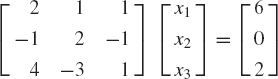
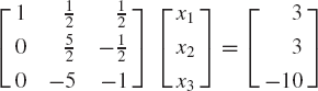
To solve for the unknowns x1, x2, and x3 using the Gaussian elimination method, we first perform the forward elimination in order to obtain an upper-triangular matrix. With this goal in mind, we multiply the first equation by ½. This leads to
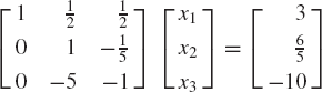
By adding the first equation to the second equation, and −4 times the first equation to the third equation, one obtains
Now we multiply the second equation by 2/5 to obtain
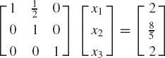
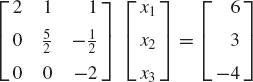
By adding 5 times the second equation to the third equation, one obtains
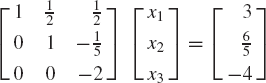
The coefficient matrix in this equation is an upper-triangular matrix and hence, the back substitution step can be used to solve for the variables. Using the third equation, one has
The first equation can then be used to solve for x1 as
Therefore, the solution of the original system of equations is
It is clear that the Gaussian elimination solution procedure reduces the system Ax = b to an equivalent system Ux = g, where U is an upper-triangular matrix. This new equivalent system is easily solved by the process of back substitution.
The Gauss-Jordan reduction method combines the forward elimination and back substitution steps. In this case, the coefficient matrix is converted to a diagonal identity matrix, and consequently, the solution is defined by the right-hand-side vector of the resulting system of algebraic equations. To demonstrate this procedure, we consider Eq. 117. Dividing the third equation by −2, one obtains
By adding 1/5 times the third equation to the second equation and −1/2 times the third equation to the first equation, one obtains
Adding −1/2 times the second equation to the first equation yields
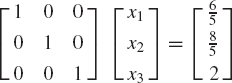
The coefficient matrix in this system is the identity matrix and the right-hand side is the solution vector previously obtained using the Gaussian elimination procedure.
It is important, however, to point out that the use of Gauss-Jordan method requires 50 percent more additions and multiplications as compared to the Gaussian elimination procedure. For an n × n coefficient matrix, the Gaussian elimination method requires approximately (n)3/3 multiplications and additions, while the Gauss-Jordan method requires approximately (n)3/2 multiplications and additions. For this reason, use of the Gauss-Jordan procedure to solve linear systems of algebraic equations is not recommended. Nonetheless, by taking advantage of the special structure of the right-hand side of the system Ax = I, the Gauss-Jordan method can be used to produce a matrix inversion program that requires a minimum storage.
It is clear that the Gaussian elimination and Gauss-Jordan reduction procedures require division by the diagonal element aii. This element is called the pivot. The forward elimination procedure at the ith step fails if the pivot aii is equal to zero. Furthermore, if the pivot is small, the elimination procedure becomes prone to numerical errors. To avoid these problems, the equations may be reordered in order to avoid zero or small pivot elements. There are two types of pivoting strategies that are used in solving systems of algebraic equations. These are the partial pivoting and full pivoting. In the case of partial pivoting, during the ith elimination step, the equations are reordered such that the equation with the largest coefficient (magnitude) of xi is chosen for pivoting. In the case of full or complete pivoting, the equations and the unknown variables are reordered in order to choose a pivot element that has the largest absolute value.
It has been observed that if the elements of the coefficient matrix A vary greatly in size, the numerical solution of the system Ax = b can be in error. In order to avoid this problem, the coefficient matrix A must be scaled such that all the elements of the matrix have comparable magnitudes. Scaling of the matrix can be achieved by multiplying the rows and the columns of the matrix by suitable constants. That is, scaling is equivalent to performing simple row and column operations. While the row operations cause the rows of the matrix to be approximately equal in magnitude, the column operations cause the elements of the vector of the unknowns to be of approximately equal size. Let C be the matrix that results from scaling the matrix A. This matrix can be written as
where B1 and B2 are diagonal matrices whose diagonal elements are the scaling constants. Hence, one is interested in solving the following new system of algebraic equations:
where
The solution of the system Cy = z defines the vector y. This solution vector can be used to define the original vector of unknowns x as
The Gaussian elimination method, in addition to being widely used for solving systems of algebraic equations, can also be used to determine the rank of nonsquare matrices and also to determine the independent variables in a given system of algebraic equations. This is demonstrated by the following example.
Example 2.12
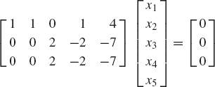
Consider the following system of algebraic equations:
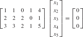
A forward elimination in the first column yields
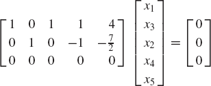
Since the coefficients of x2 in the second and third equations are equal to zero, these coefficients cannot be used as pivots in the Gaussian elimination. By using an elementary column operation, the second and third columns can be interchanged leading to a reordering of the variables. Such an elementary operation yields

Dividing the second row by 2 and performing forward elimination in the second column yields
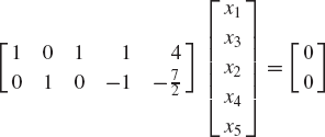
The coefficient matrix in this equation has two independent rows and, consequently, its rank is equal to two. This is an indication that there are only two independent equations. One can then disregard the third equation and use the following system of equations:
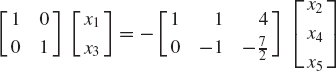
It is clear from this equation that x1 and x3 can be determined if the values of x2, x4, and x5 are given. Therefore, x2, x4, and x5 are called the independent variables, while x1 and x3 are called the dependent variables.
In the Gaussian elimination procedure used to solve the system Ax = b, the n × n coefficient matrix reduces to an upper-triangular matrix after n − 1 steps. The new system resulting from the forward elimination can be written as
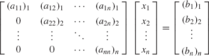
where ( )k refers to step k in the forward elimination process and
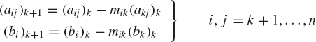
and
Let U denote the upper-triangular coefficient matrix in Eq. 122 and define the lower-triangular matrix L as
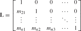
where the coefficients Mij are defined by Eq. 124. Using Eqs. 123 and 124, direct matrix multiplication shows that the matrix A can be written as
which implies that the matrix A can be written as the product of a lower-triangular matrix L and an upper-triangular matrix U.
Example 2.13
The lower-triangular matrix L can also be defined using the elementary operations of Gaussian elimination. In order to demonstrate this, we consider the system
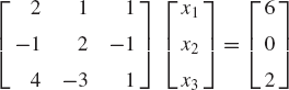
whose solution was obtained in the preceding section using Gaussian elimination. In order to solve this system, the following three elimination steps are used.
Add 1/2 times the first equation to the second equation.
Subtract 2 times the first equation from the third equation.
Add 2 times the second equation to the third equation.
The result of these three elementary operations is an equivalent but simpler system given by
in which the upper-triangular matrix U can be recognized as
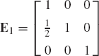
Elementary operations can also be performed using elementary matrices. An elementary matrix is obtained by performing the elementary operation on an identity matrix. Premultiplying the coefficient matrix A by an elementary matrix produces the same elementary operation for A. For instance, if 1/2 times the first row of a 3 × 3 identity matrix is added to the second row, one obtains the elementary matrix
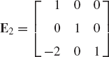
Also, if 2 times the first row of a 3 × 3 identity matrix is substracted from the third row, one obtains the elementary matrix
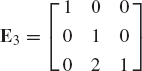
Similarly, if 2 times the second row is added to the third row, one obtains the elementary matrix
The product of the three elementary matrices E3, E2, and E1 is
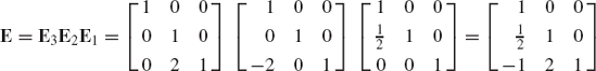
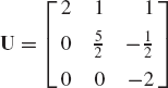
Note that E is a lower-triangular matrix with all the diagonal elements equal to 1. Note also that premultiplying the coefficient matrix A by E leads to
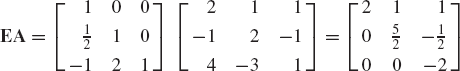
which is the same upper-triangular matrix U obtained previously by the elementary operations of Gaussian elimination. The diagonal elements of the matrix U are the pivots. Therefore, one has
or
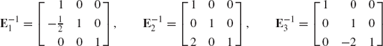
where E−1 = (E3E2E1)−1 = E−11E−12E−13 is the matrix L that defines the LU factorization of the matrix A. The inverse of an elementary matrix is also an elementary matrix. The inverses of the matrices E1, E2, and E3 are defined as
It follows that

While Eqs. 122 through 126 present the LU factorization resulting from the use of Gaussian elimination, we should point out that in general such a decomposition is not unique. The triangular matrix L obtained by using the steps of Gaussian elimination has diagonal elements that are all equal to 1. The method that gives explicit formulas for the elements of L and U in this special case is known as Doolittle's method. If the upper-triangular matrix U is defined such that all its diagonal elements are equal to 1, we have Crout's method. Obviously, there is only a multiplying diagonal matrix that distinguishes between Crout's and Doolittle's methods. To demonstrate this, let us assume that A has the following two different decompositions:
It is then clear that
Since the inverse and product of lower (upper)-triangular matrices are again lower (upper) triangular, the left and right sides of Eq. 128 must be equal to a diagonal matrix D, that is,
It follows that
which demonstrate that there is only a multiplying diagonal matrix that distinguishes between two different methods of decomposition.
A more efficient decomposition can be found if the matrix A is symmetric and positive definite. The matrix A is said to be positive definite if xT AX > 0 for any n-dimensional nonzero vector x. In the case of symmetric positive definite matrices, Cholesky's method can be used to obtain a simpler factorization for the matrix A. In this case, there exists a lower-triangular matrix L such that
where the elements lij of the lower-triangular matrix L can be defined by equating the elements of the products of the matrices on the right side of Eq. 131 to the elements of the matrix A. This leads to the following general formulas for the elements of the lower-triangular matrix L:
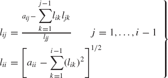
Cholesky's method requires only
Once the decomposition of A into its LU factors is defined, by whatever method, the system of algebraic equations
can be solved by first solving
and then solve for x using the equation
The coefficient matrices in Eqs. 134 and 135 are both triangular and, consequently, the solutions of both equations can be easily obtained by back substitution.
We should point out that the accuracy of the solution obtained using the direct methods such as Gaussian elimination and other LU factorization techniques depends on the numerical properties of the coefficient matrix A. A linear system of algebraic equations Ax = b is called ill-conditioned if the solution x is unstable with respect to small changes in the right-side b. It is important to check the effectiveness of the computer programs used to solve systems of linear algebraic equations when ill-conditioned problems are considered. An example of an ill-conditioned matrix that can be used to evaluate the performance of the computer programs is the Hilbert matrix. A Hilbert matrix of order n is defined by
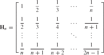
The inverse of this matrix is known explicitly. Let cij be the ijth element in the inverse of Hn. These elements are defined as
The Hilbert matrix becomes more ill-conditioned as the dimension n increases.
Another important matrix factorization that is used in the computational dynamics of mechanical systems is the QR decomposition. In this decomposition, an arbitrary matrix A can be written as
where the columns of Q are orthogonal and R is an upper-triangular matrix. Before examining the factorization of Eq. 138, some background material will first be presented.
In Section 3, the orthogonality of n-dimensional vectors was defined. Two vectors a and b are said to be orthogonal if aTb = 0. Orthogonal vectors are linearly independent, for if a1, a2, ..., an is a set of nonzero orthogonal vectors, and
one can multiply this equation by aTi and use the orthogonality condition to obtain αiaTiai = 0. This equation implies that αi=0 for any i. This proves that the orthogonal vectors a1, a2, ..., an are linearly independent. In fact, one can use any set of linearly independent vectors to define a set of orthogonal vectors by applying the Gram-Schmidt orthogonalization process.
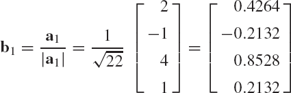
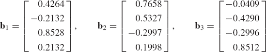
Let a1, a2, ..., am be a set of n-dimensional linearly independent vectors where m ≤ n. To use this set of vectors to define another set of orthogonal vectors B1, b2, ..., bm, we first define the unit vector
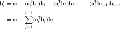
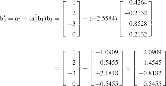
Recall that the component of the vector a2 in the direction of the unit vector b1 is defined by the dot product aT2b1. For this reason, we define b'2 as
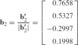
Clearly, b'2 has no component in the direction of b1 and, consequently, b1 and b'2 are orthogonal vectors. This can simply be proved by using the dot product bT1b'2 and utilizing the fact that b1 is a unit vector. Now the unit vector b2 is defined as
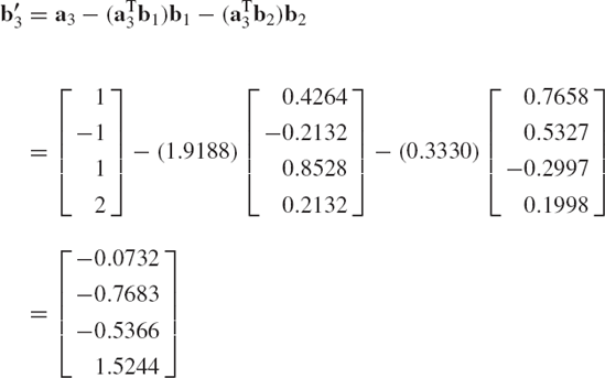
Similarly, in defining b3 we first eliminate the dependence of this vector on b1 and b2. This can be achieved by defining
The vector b3 can then be defined as
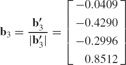
Continuing in this manner, one has
and
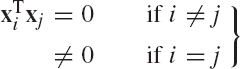
As the result of the application of the Gram-Schmidt orthogonalization process one obtains a set of orthonormal vectors that satisfy
The Gram-Schmidt orthogonalization process cannot be completed if the vectors are not linearly independent. In this case, it is impossible to obtain a set that consists of only nonzero orthogonal vectors.
Example 2.14
Consider the linearly independent vectors defined by the columns of the rectangular matrix
Let
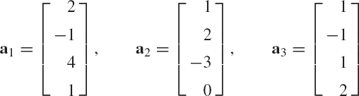
In order to define a set of orthogonal vectors, we first define
The vector b'2 is
The vector b2 can then be defined as
The vector b'3 is defined as
Therefore, the vector b3 is
The three orthonormal vectors are

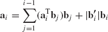
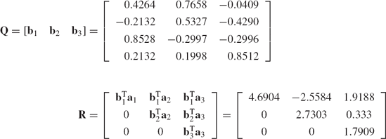
The Gram-Schmidt orthogonalization process can be used to demonstrate that an arbitrary rectangular matrix A with linearly independent columns can be expressed in the following factored form A = QR of Eq. 138, where the columns of Q are orthogonal or orthonormal vectors and R is an upper-triangular matrix. To prove Eq. 138, we consider the n × m rectangular matrix A. If a1, a2, ..., am are the columns of A, the matrix A can be written as
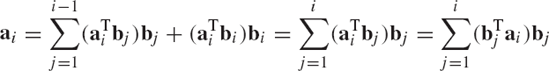
If the n-dimensional vectors a1, ..., and am are linearly independent, the Gram-Schmidt orthogonalization procedure can be used to define a set of m orthogonal vectors b1, b2, ..., and bm as previously described in this section. Note that in Eq. 138, the columns of A are a linear combination of the columns of Q. Thus, to obtain the factorization of Eq. 138, we attempt to write a1, a2, ..., am as a combination of the orthogonal vectors b1, b2, ..., bm. From Eqs. 145 and 146, one has
Since b1, b2, ..., and bm are orthonormal vectors, the use of Eq. 149 leads to
Substituting Eq. 150 into Eq. 149, one gets
Using this equation, the matrix A, which has linearly independent columns, can be written as
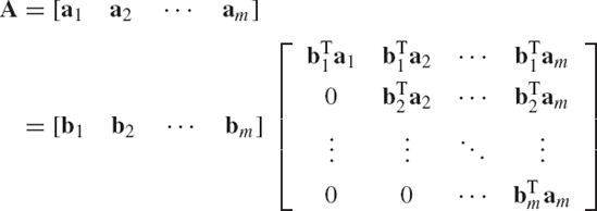
which can also be written as A = QR, where
and
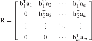
The matrix Q is an n × m matrix that has orthonormal columns. The m × m matrix R is an upper triangular and is invertible.
If A is a square matrix, the matrix Q is square and orthogonal. If the Q and R factors are found for a square matrix, the solution of the system of equations Ax = b can be determined efficiently, since in this case we have QRx = b or Rx = QTb. The solution of this system can be obtained by back-substitution since R is an upper-triangular matrix.
The application of the Gram-Schmidt orthogonalization process leads to a QR factorization in which the matrix Q has orthogonal column vectors, while the matrix R is a square upper-triangular matrix. In what follows, we discuss a procedure based on the Householder transformation. This procedure can be used to obtain a QR factorization in which the matrix Q is a square orthogonal matrix.
A Householder transformation or an elementary reflector associated with a unit vector
where I is an identity matrix. The matrix H is symmetric and also orthogonal since
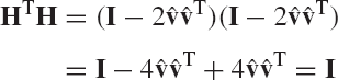
It follows that H = HT = H−1. It is also clear that if
Furthermore, if u is the column vector
and
where
then
Using Eq. 159, one obtains
Since
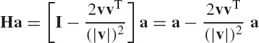
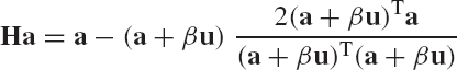
the denominator in Eq. 162 can be written as (a + βu)T(a + βu) = 2(a + βu)Ta. Substituting this equation into Eq. 162 yields

This equation implies that when the Householder transformation constructed using the vector v of Eq. 159 is multiplied by the vector a, the result is a vector whose only nonzero element is the first element. Using this fact, a matrix can be transformed to an upper-triangular form by the successive application of a series of Householder transformations. In order to demonstrate this process, consider the rectangular n × m matrix
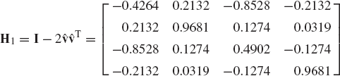
where n ≥ m. First we construct the Householder transformation associated with the first column a1=[a11 a21 ... an1]T. This transformation matrix can be written as
where the vector v1 is defined as
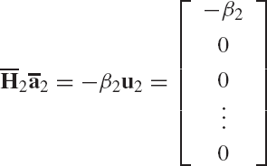
in which β1 is the norm of a1, and the vector u1 has the same dimension as a1 and is defined by Eq. 158. Using Eq. 164, it is clear that
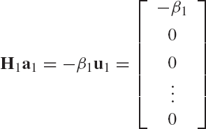
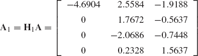
It follows that
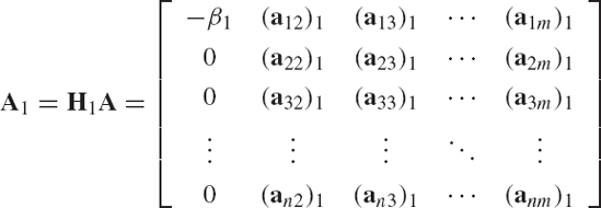
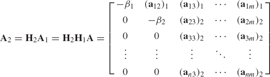
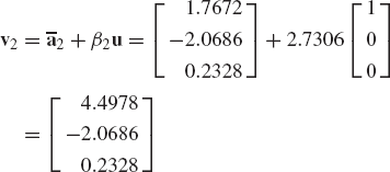
Now we consider the second column of the matrix A1 = H1A. We use the last n − 1 elements of this column vector to form
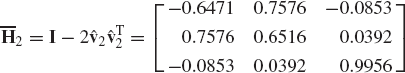
A Householder transformation matrix
where β2 is the norm of the vector ā2, and u2 is an (n − 1)-dimensional vector defined by Eq. 158. Observe that at this point, the Householder transformation
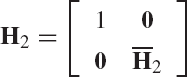
Because only the first element in the first row and first column of this matrix is nonzero and equal to 1, when this transformation is applied to an arbitrary matrix it does not change the first row or the first column of that matrix. Furthermore, H2 is an orthogonal symmetric matrix, since
We consider the third column of the matrix A2, and use the last n − 2 elements to form the vector
The Householder transformation
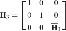
Using this matrix, one has
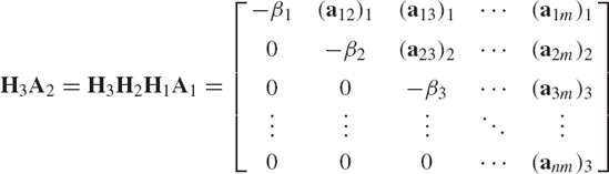
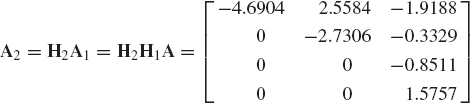
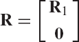
where β3 is the norm of the vector ā3. It is clear that by continuing this process, all the elements below the diagonal of the matrix A can be made equal to zero. If A is a square nonsingular matrix, the result of the Householder transformations is an upper-triangular matrix. If A, on the other hand, is a rectangular matrix, the result of m-Householder transformations is
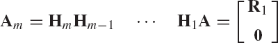
where R1 is an m × m upper-triangular matrix.
Example 2.16
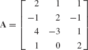
Consider the matrix
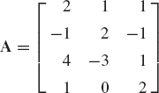
First we consider the first column of this matrix:
The norm of this vector is
The vector v1 is defined as
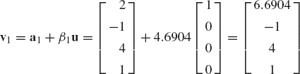
The unit vector
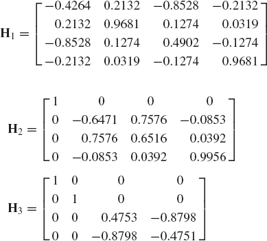
The Householder transformation H1 is
The matrix A1 is
The vector ā2 can be obtained from the second column of this matrix as
The norm of this vector is
The vector v2 is defined as
It follows that
The matrix
The matrix H2 can be written as

and
Using the last two elements of the third column of this matrix, one defines
The norm of this vector is
The vector v3 is defined as
A unit vector in the direction of v3 is
The Householder transformation associated with this vector is
Using this matrix, the transformation H3 can be defined as
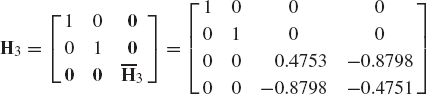
Using this matrix, one obtains

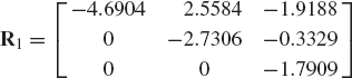
The matrix A3 can be written as
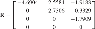
where R1 is the upper-triangular matrix
Note the relationship between the matrix R1 obtained in this example by the successive application of Householder transformations and the matrix R obtained in Example 15 as the result of the application of the Gram-Schmidt orthogonalization process. The similarity between these two matrices is not surprising because the uniqueness of the QR factorization can easily be demonstrated.
The application of a sequence of Householder transformations to an n × m rectangular matrix A with linearly independent columns leads to
where Hi is the ith orthogonal Householder transformation and R is an n × m rectangular matrix that can be written as
where R1 is an m × m upper-triangular matrix. If A is a square matrix, R = R1. Since the Householder transformations are symmetric and orthogonal, one has
Using this identity, Eq. 178 leads to
Since the product of orthogonal matrices defines an orthogonal matrix, Eq. 181 can be written in the form of Eq. 138 as A = QR, where Q is an orthogonal square matrix defined as
Example 2.17
In the preceding example it was shown that the Householder transformations that reduce the matrix
to the matrix
are
In this case, the matrix Q of Eq. 182 is
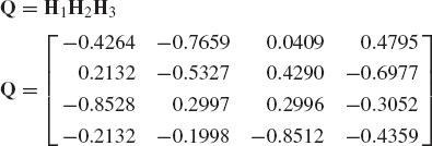
The similarity between the first three columns of this matrix and the matrix Q obtained in Example 15 using the Gram-Schmidt orthogonalization process is clear.
If the fourth column of the preceding matrix is denoted as Q2, that is,
it is easy to verify that ATQ2 = 0.
If A is an n × m rectangular matrix that has the QR decomposition given by Eq. 138, the matrix R takes the form given by Eq. 179. In this case, one can use matrix partitioning to write
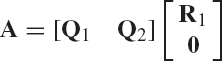
where Q1 and Q2 are partitions of the matrix Q, that is,
The matrix Q1 is an n × m matrix, while Q2 is an n × (n−m) matrix. Both Q1 and Q2 have columns that are orthogonal vectors. Furthermore,
It follows from Eq. 183 that
Consequently,
If A has linearly independent columns, Eq. 187 represents the Cholesky factorization of the positive definitive symmetric matrix ATA. Therefore, R1 is unique. The uniqueness of Q1 follows immediately from Eq. 186, since
While Q1 and R1 are unique, Q2 is not unique. We note, however, that
or
which implies that the orthogonal column vectors of the matrix Q2 form the basis of the null space of the matrix AT. This fact was demonstrated by the results presented in Example 17.
Another factorization that is used in the dynamic analysis of mechanical systems is the singular value decomposition (SVD). The singular value decomposition of the matrix A can be written as
where Q1 and Q2 are two orthogonal matrices and B is a diagonal matrix which has the same dimension as A. Before we prove Eq. 191, we first discuss briefly the eigenvalue problem.
In mechanics, we frequently encounter a system of equations in the form
where A is a square matrix, x is an unknown vector, and λ is an unknown scalar. Equation 192 can be written as
This system of equations has a nontrivial solution if and only if the determinant of the coefficient matrix is equal to zero, that is,
This is the characteristic equation for the matrix A. If A is an n × n matrix, Eq. 194 is a polynomial of order n in λ. This polynomial can be written in the following general form:
where ak are the coefficients of the characteristic polynomial. The solution of Eq. 195 defines the n roots λ1, λ2, ..., λn. The roots λi, i = 1, ..., n are called the characteristic values or the eigenvalues of the matrix A. Corresponding to each of these eigenvalues, there is an associated eigenvector xi, which can be determined by solving the system of homogeneous equations
If A is a real symmetric matrix, one can show that the eigenvectors associated with distinctive eigenvalues are orthogonal. To prove this fact, we use Eq. 196 to write
Premultiplying the first equation in Eq. 197 by xTj and postmultiplying the transpose of the second equation by xi, one obtains
Subtracting yields
which implies that
This orthogonality condition guarantees that the eigenvectors associated with distinctive eigenvalues are linearly independent.
Example 2.18
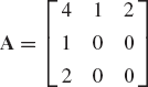
Find the eigenvalues and eigenvectors of the matrix
Solution. The characteristic equation of this matrix is
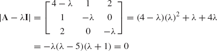
Therefore, the eigenvalues are
To evaluate the ith eigenvector, one may use the following equation:
where xi is the ith eigenvector. The preceding equation can be written as
which yields the following eigenvectors:
These eigenvectors are orthogonal because the matrix A is real and symmetric. We also observe that the resulting eigenvalues are all real. It can be shown that if A is a real symmetric matrix, then all its eigenvalues and eigenvectors are real.
Equation 192 indicates that the eigenvectors are not unique since this equation remains valid if it is multiplied by an arbitrary nonzero scalar. In the case of a real symmetric matrix, if each of the eigenvectors is divided by its length, one obtains an orthonormal set of vectors denoted as
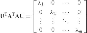
An orthogonal matrix whose columns are the orthonormal eigenvectors
From Eq. 201, it follows that
Example 2.19
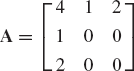
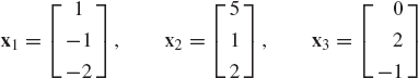
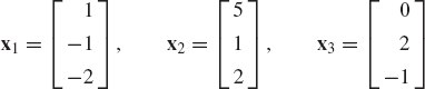
It was shown in the preceding example that the eigenvalues of the real symmetric matrix
are λ1 = −1, λ2 = 5, and λ3 = 0. The eigenvectors associated with these eigenvalues were found to be
An orthonormal set of eigenvectors can be obtained by dividing each eigenvector by its length. This leads to
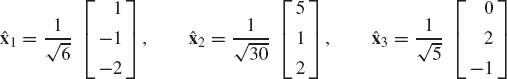
The orthonormal matrix U of Eq. 202 can then be defined as
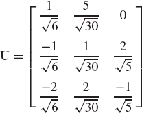
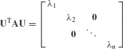
Matrix multiplications show that
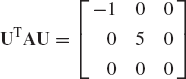
The zero eigenvalue that appears as the last element of the diagonal of the matrix UT AU indicates a rank deficiency of the matrix A since the second and third rows of the matrix A are not linearly independent. The rank of this matrix is 2.
In the singular value decomposition of Eq. 191, A can be an arbitrary n × m rectangular matrix. In this case Q1 is an n × n matrix, B is an n × m matrix, and Q2 is an m × m matrix. To prove the decomposition of Eq. 191, we consider the real symmetric square matrix AT A. The eigenvalues of AT A are real and nonnegative. To demonstrate this, we assume that
It follows that
and also
It is clear from the preceding two equations that
which demonstrates that λ is indeed nonnegative and AT Ax = 0 if and only if Ax = 0.
It was demonstrated previously in this section that if
where λ1, λ2, ..., λm are the eigenvalues of the matrix AT A. Equation 208 implies that the columns b1, b2, ..., bm of the matrix AU satisfy
For the r nonzero eigenvalues, where r ≤ m, we define
This is an orthonormal set of vectors. If r < m and n ≥ m, we choose
is an n × n orthogonal matrix. Recall that AU=[b1 b2 ... bm]. Using this equation and Eq. 210, it can be verified that
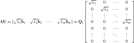
or A = Q1BQ2, where Q2 = UT, and B is the n × m matrix
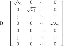
This completes the proof of Eq. 191.
Example 2.20
Find the singular value decomposition of the matrix
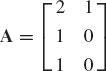
Solution. The matrix AT A is a 2 × 2 matrix that can be calculated as
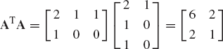
The characteristic polynomial of this matrix is
from which the eigenvalues can be determined as
The eigenvectors are
The orthonormal eigenvectors are
The matrix U is then defined as
It follows that
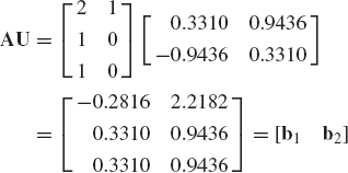
The orthonormal vectors
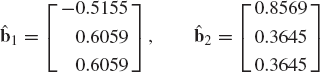
The matrix Q1 can then be defined as
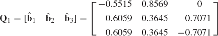
and the matrix Q2 is
The matrix B that contains the singular values is
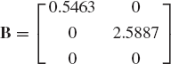
Therefore, the matrix A can be written as A = Q1BQ2.
Using the factorization of Eq. 191, one has
which implies that the columns of the matrix Q1 are eigenvectors of the matrix AAT and the square of the diagonal elements of the matrix B are the eigenvalues of the matrix AAT. That is, the eigenvalues of AT A are the same as those of AAT. The eigenvectors, however, are different since
which implies that the rows of Q2 are eigenvectors of AT A. These conclusions can be verified using the results obtained in Example 20.
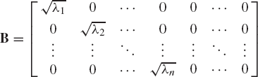
The matrix B, whose diagonal elements are the square roots of the eigenvalues of the matrix AT A, takes the form of Eq. 213 if the number of rows of the matrix A is greater than the number of columns (n > m). If n < m, the matrix B takes the form
where the number of zero columns in this matrix is m − n. This fact is also clear from the definition of the transpose of the rectangular matrix A, for if the singular value decomposition of a rectangular matrix A is given by Eq. 191, the singular value decomposition of its transpose is given by
Now let us consider the singular value decomposition of the n × m rectangular matrix where n>m. The matrix B of Eq. 213 can be written as
where B1 is a diagonal matrix whose elements, the singular values, are the square roots of the eigenvalues of the matrix ATA. Using the partitioning of Eq. 217, Eq. 191 can be written in the following partitioned form:
where Q1d and Q1i are partitions of the matrix Q1. The columns of the matrices Q1d and Q1i are orthogonal vectors, and
It follows from Eq. 219 that
Multiplying this equation by QTli and using the results of Eq. 220, one obtains
which implies that the orthogonal columns of the matrix Q1i span the null space of the matrix AT. In the dynamic analysis of multibody systems, Eq. 222 can be used to obtain a minimum set of independent differential equations that govern the motion of the interconnected bodies in the system.
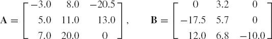
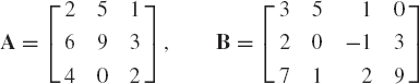
Find the sum of the following two matrices:
Evaluate also the determinant and the trace of A and B.
Find the product AB and BA, where A and B are given in problem 1.
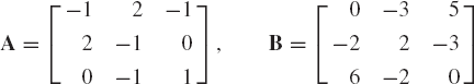
Find the inverse of the following matrices.
Show that an arbitrary square matrix A can be written as
where A1 is a symmetric matrix and A2 is a skew-symmetric matrix.
Show that the interchange of any two rows or columns of a square matrix changes only the sign of the determinant.
Show that if a matrix has two identical rows or two identical columns, the determinant of this matrix is equal to zero.
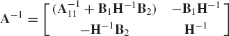
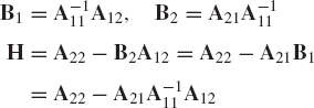
Let
be a nonsingular matrix. If A11 is square and nonsingular show by direct matrix multiplications that
where
Using the identity given in problem 7, find the inverse of the matrices A and B given in problem 3.
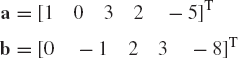
Let a and b be the two vectors
Find a + b, a · b, |A|, and |b|.
Find the total derivative of the function
with respect to the parameter t. Define also the partial derivative of the function f with respect to the vector q(t) where
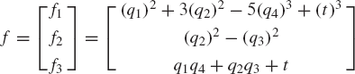
Find the total derivative of the vector function
with respect to the parameter t. Define also the partial derivative of the function f with respect to the vector
Let Q = qT Aq, where A is an n × n square matrix and q is an n-dimensional vector. Show that
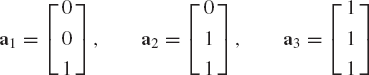
Show that the vectors
are linearly independent. Determine also the coordinates of the vector b = [1 −5 3]T in the basis a1, a2, and a3.
Find the rank of the following matrices:
Find the cross product of the vectors a = [1 0 3]T and b = [9 −3 1]T. If c = a×b, verify that cTa = cTb =0.
Show that if a and b are two parallel vectors, then a × b = 0.
Show that if a and b are two orthogonal vectors and c = a×b, then |c|=|a| |b|.
Find the skew-symmetric matrices associated with the vectors
Using these skew-symmetric matrices, find the cross product a × b and b × a.
Find the solution of the homogeneous system of equations a × x = 0, where a is the vector a = [−2 5 −9]T.
Find the solution of the system of homogeneous equations a × x = 0, where a is the vector a =[−11 −3 4]T.
If a = [a1 a2 a3]T and b = [b1 b2 b3]T are given vectors, show using direct matrix multiplication that
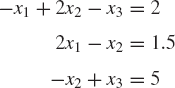
Find the solution of the following system of algebraic equations:
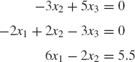
Find the solution of the following system of equations:
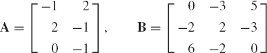
Use the Gram-Schmidt orthogonalization process to determine the QR decomposition of the matrices
Use the Householder transformations to solve problem 24.
Determine the singular value decomposition of the matrices A and B of problem 24.
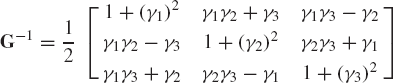
Prove that the determinant of the matrix
is 2, where (γ)2 = (γ1)2 + (γ2)2 + (γ3)2. Prove also that the inverse of the matrix G is
Show that the matrix A = G(G−1)T is an orthogonal matrix. Show also that the vector
is an eigenvector for the matrix A and determine the corresponding eigenvalue.
Prove the polar decomposition theorem, which states that a nonsingular square matrix A can be uniquely decomposed into A = QV1 or A = V2Q, where Q is an orthogonal matrix and v1 and v2 are positive-definite symmetric matrices.