In this chapter, several topics in dynamics are presented. In the first section, the use of Euler angles to study the gyroscopic motion is discussed. In the following sections, several alternative methods for defining the orientations of the rigid bodies in space are presented. In Section 2, the Rodriguez formula, which is expressed in terms of the angle of rotation and a unit vector along the axis of rotation, is presented. Euler parameters, which are widely used in general-purpose multibody computer programs to avoid the singularities associated with Euler angles, are introduced in Section 3. Rodriguez parameters are discussed in Section 4 for the sake of completeness. Euler parameters can be considered as an example of the quaternions, which are introduced in Section 5. In Section 6, the problem of nonimpulsive contact between rigid bodies is discussed. A method for the stability and eigenvalue analysis of constrained multibody system is presented in Section 7.
The study of the gyroscopic motion is one of the most interesting problems in spatial dynamics. This problem occurs when the orientation of the axis of rotation of a rigid body changes. The gyroscope shown in Fig. 1 consists of a rotor that spins about its axis of rotational symmetry Z3 which is mounted on a ring called the inner gimbal. As shown in the figure, the rotor is free to rotate about its axis of symmetry relative to the inner gimbal, and the inner gimbal rotates freely about the axis X2, which is perpendicular to the axis of the rotor. The axis X2 is mounted on a second gimbal, called the outer gimbal, which is free to rotate about the axis Z1. The rotor whose center of gravity remains fixed may attain any arbitrary position as shown in Fig. 1 by the following three successive rotations.
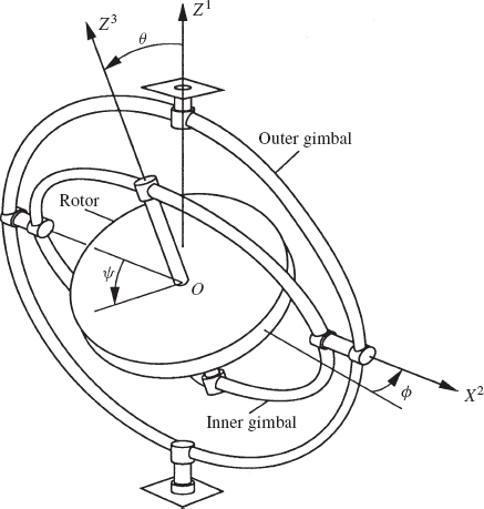
A rotation ϕ of the outer gimbal about the axis Z1.
A rotation θ of the inner gimbal about the axis X2.
A rotation ψ of the rotor about its own axis Z3.
These three Euler angles are called the precession, the nutation, and the spin, and the type of mounting used in the gyroscope is called a cardan suspension.
The angular velocity of the rotor can be written as
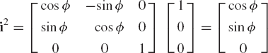
where k1 is a unit vector along the Z1 axis, i2 is a unit vector along the X2 axis, and k3 is a unit vector along the Z3 axis. The unit vector k1 is
Since the rotation ϕ is about the Z1 axis, the unit vector i2 is defined as
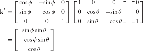
Since the rotation θ is about the X2 axis, the unit vector k3 is defined as
The angular velocity of the rotor can then be written as
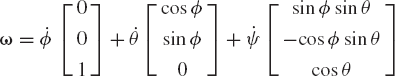
which can be written in a matrix form as
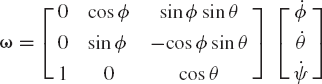
This equation can be written as
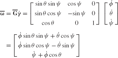
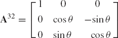
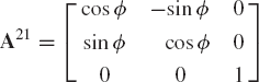
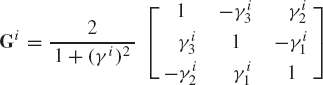
where G is the matrix whose columns are the unit vectors k1, i2, and k3. This matrix was previously defined in terms of Euler angles in the preceding chapter as
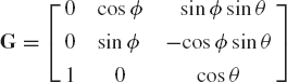
and
Differentiating the angular velocity vector with respect to time, one obtains the absolute angular acceleration vector α of the rotor as
where

The equations of motion of the rotor of the gyroscope can be conveniently derived using Lagrange's equation. To this end, we first define the angular velocity vector in the rotor coordinate system as
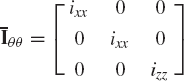
Because of the symmetry of the rotor about its X3 axis, its products of inertia are equal to zero, and ixx = iyy. The inertia tensor of the rotor defined in the rotor coordinate system is
Since the center of mass of the rotor is fixed, the kinetic energy of the rotor is given by
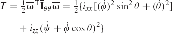
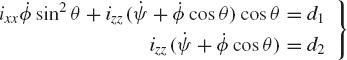
Using the Eulerian angles ϕ, θ, and ψ as the generalized coordinates of the rotor, the equations of motion of the rotor are given by
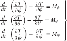
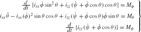
where Mϕ, Mθ and Mψ are the components of the generalized applied torque associated with the angles ϕ, θ, and ψ, respectively. Using the expression previously obtained for the kinetic energy, one can show that the equations of motion of the rotor are
In what follows, several important special cases are discussed.
It can be seen that the kinetic energy of the rotor is not an explicit function of the precession and spin angles ϕ and ψ, that is,
If the torques Mϕ and Mψ are equal to zero, Lagrange's equation yields
or
where d1 and d2 are constants. In this special case, the precession and spin angles ϕ and ψ are called ignorable coordinates since the generalized momentum associated with these coordinates is conserved. The use of the preceding equations yields the following integrals of motion:
where the constants d1 and d2 can be determined using the initial conditions. In this special case, the equation for the nutation angle θ can be written as
Consider the special case in which the rotor precesses at a steady rate
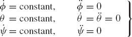
In this case, the equations of the rotor reduce to
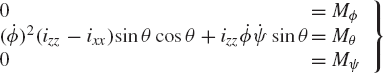
It is clear that in this case Mϕ = Mψ = 0, and the only nonzero torque acting on the rotor is the constant torque associated with the nutation angle θ. The axis of this torque is perpendicular to the axis of precession. If we further assume that θ = π/2, the torque Mθ takes the simple form
Euler's theorem states that the most general displacement of a body with one point fixed is a rotation about an axis called the instantaneous axis of rotation. According to this theorem, the coordinate transformation can be defined by a single rotation about the instantaneous axis of rotation. The components of a unit vector along the instantaneous axis of rotation as well as the angle of rotation of the rigid body about this axis can be used to develop the transformation matrix that defines the body orientation. The obtained transformation matrix, in this case, is expressed in terms of four parameters; the three components of the unit vector along the instantaneous axis of rotation and the angle of rotation.
Figure 2 shows the initial position of a vector
It can be shown that (Shabana, 1998)
It follows that
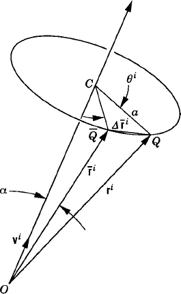
Using the skew-symmetric matrix notation, the vector ri can be written as
which can also be written as
where Ai is the transformation matrix defined in terms of the unit vector vi and the rotation angle θi as
This equation, which is called Rodriguez formula, is expressed in terms of the four parameters νi1, νi2, νi3, and θi which are not totally independent since
The components of the angular velocity vector ωi of the rigid body i can be defined using the relationship,
from which
which can be expressed in a matrix form as
where
Similarly, the components of the angular velocity vector of the rigid body i defined in the body coordinate system can be obtained using the relationship
from which
which can also be written in a matrix form as
where
Equations 32 and 36 clearly demonstrate that the magnitude of the angular velocity is
If the axis of rotation is parallel to one of the axes of the coordinate system, the use of Rodriguez formula leads to the definition of the simple rotation matrices defined in the preceding chapter. Interestingly, Rodriguez formula suggests that there are two different procedures for solving the problem of successive rotations. In order to illustrate the use of these two different procedures, we consider the robotic manipulator shown in Fig. 3. It is clear from this figure that the orientation of object 4 with respect to link 3 is defined by the transformation matrix
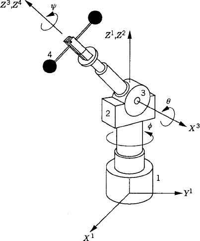
The orientation of link 3 with respect to link 2 is defined by the transformation matrix
and the orientation of link 2 with respect to link 1 is
The transformation matrix that defines the orientation of object 4 with respect to the fixed link (link 1) can then be written as
Matrix multiplications show that the matrix A41 takes the same form as the Euler angle transformation matrix given in the preceding chapter.
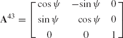
Using the Rodriguez formula, a different procedure can be used to define the orientation of object 4. In this procedure, the joint axes of rotations are defined in the fixed coordinate system as
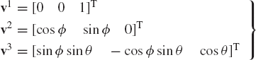
Using these three unit vectors, the following three transformation matrices are defined:
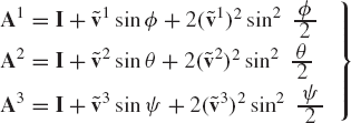
It is left to the reader as an exercise to show that the transformation matrix A41 can also be defined as
This sequence of transformations differs from the sequence discussed previously in the sense that after each rotation the orientation of the body is redefined in the fixed coordinate system using Rodriguez formula (Shabana, 1998).
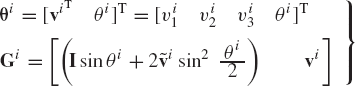
An alternative set of four parameters that can be used to describe the orientation of the rigid bodies is the set of Euler parameters. The four Euler parameters can be expressed in terms of the components of the unit vector along the instantaneous axis of rotation as well as the angle of rotation as
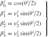
The four Euler parameters are not totally independent since
Using Rodriguez formula, the transformation matrix Ai can be expressed in terms of Euler parameters as
where
The transformation matrix can be written explicitly in terms of Euler parameters as
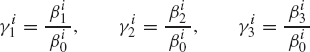
In terms of Euler parameters, the angular velocity vector of the rigid body i is defined as
where
The angular velocity vector defined in the body coordinate system is
where
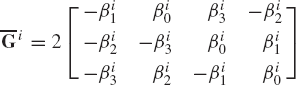
The transformation matrix Ai can be expressed in terms of the matrices Gi and
Note also that
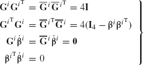
where I4 is the 4 × 4 identity matrix. Differentiating Eqs. 51 and 53 and using the identities of Eq. 56, it can be shown that the angular acceleration vectors can be expressed in terms of Euler parameters as
Clearly, Euler parameters have one redundant variable since they are related by Eq. 47. Nonetheless, Euler parameters are used in several general-purpose multibody computer programs because they do not suffer from the singularity problem associated with the three-parameter representation. Euler parameters are also bounded because they are defined in terms of sine and cosine functions. Moreover, the time derivatives of Euler parameters can be determined at any configuration of the rigid body, if the angular velocity vector is given. This is demonstrated by the following example.
Example 8.1
The orientation of a rigid body is defined by the four Euler parameters
At the given configuration, the body has an instantaneous angular velocity defined in the global coordinate system by the vector
Find the time derivatives of Euler parameters.
Solution. Using Eq. 51, one has
Multiplying both sides of this equation by GiT and using the identities of Eq. 56, one obtains
which yields
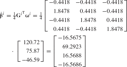
This solution must satisfy the identity
Using Euler parameters given in this example, one can show that the transformation matrix Ai is
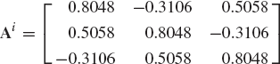
Using this transformation matrix, it can be shown that the angular velocity vector defined in the body coordinate system is
The time derivatives of Euler parameters can also be evaluated using the relationship
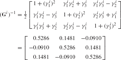
In Rodriguez formula and in the case of Euler parameters, the transformation matrix is expressed in terms of four parameters. It was demonstrated in the preceding chapter that the transformation matrix can be expressed in terms of the three independent Euler angles. In what follows, an alternate representation that uses three parameters called Rodriguez parameters, is developed. The three Rodriguez parameters are defined in terms of the components of a unit vector along the axis of rotation and the angle of rotation as
That is
Using the definitions of the preceding equation and the Rodriguez formula of Eq. 29, one obtains the transformation matrix expressed in terms of Rodriguez parameters as
where γ− i is the skew symmetric matrix associated with the vector γi and
The angular velocity vectors can be expressed in terms of Rodriguez parameters as
where
and
Example 8.2
The orientation of a rigid body is defined by the four Euler parameters
At the given configuration, the body has an instantaneous absolute angular velocity defined by the vector
Find the time derivatives of Rodriguez parameters.
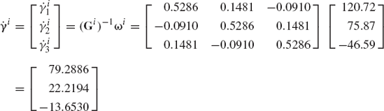
Solution. Rodriguez parameters at the given orientation are
Using the values of Euler parameters given in this example, one has
Recall that
where
The time derivatives of Rodriguez parameters can then be expressed in terms of the angular velocity as
where
The time derivatives of Rodriguez parameters are
Quaternion algebra can be used to study the rotations of the rigid bodies in space. This algebra can serve as a convenient way for describing the relative rotations between different bodies. For instance, Euler parameters discussed previously in this chapter can be considered as an example of the quaternions. Before demonstrating the use of the quaternions to describe the three-dimensional rotations, a brief introduction to quaternion algebra is presented (Megahed, 1993).
A quaternion qt is defined using a scalar and a vector as follows:
where s is a scalar, i, j, and k are unit vectors along three perpendicular Cartesian axes, and v is the vector which is defined as
Given two quaternion qt1 and qt2 defined as
quaternion addition and subtraction follows the rule
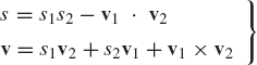
The multiplication of the quaternions is noncommutative and follows the rule
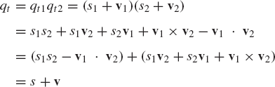
where (.) indicates a dot product, × indicates a cross product, and the scalar s and the vector v are defined as
The conjugate of the quaternion qt is defined as
The norm of the quaternion qt is defined as
Using the rule of multiplication of the quaternions, it can be shown that
If the scalar part of the quaternion is equal to zero, the quaternion norm reduces to the definition of the length of vectors used in conventional vector algebra.
The set of Euler parameters can be considered as a quaternion with a unit norm. This fact can easily be demonstrated by writing the set of Euler parameters of a rigid body or a frame of reference i in the following quaternion form:
where the scalar and vector components of this quaternion are defined in Section 3. The conjugate of the quaternion defined in the preceding equation is
and its norm is
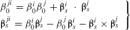
If A1, A2, and A3 are three orthogonal transformation matrices defined in terms of the sets of Euler parameters (β10, β1s), (β20, β2s), and (β30, β3s), respectively, matrix multiplication and quaternion multiplication are in one-to-one correspondence; that is, if
then
or
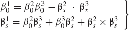
This important result from quaternion algebra can be used to study the relative motion between rigid bodies or coordinate systems. For instance, let Ai and Aj be the transformation matrices that define the orientation of two coordinate systems i and j, respectively, and let Aji be the matrix that defines the orientation of the coordinate system j with respect to the coordinate system i. It follows that
or
Recall that if (βi0, βis) is the set of Euler parameters of Ai, the set of Euler parameters associated with the transpose of Ai is (βi0, −βis) (Shabana, 1998). It follows that the set of Euler parameters associated with the relative transformation matrix Aji can easily be obtained using the quaternion algebra as
As an example that illustrates the use of the preceding equations, we assume that body j rotates with respect to body i with a constant angular velocity ωji. It follows from the first equation of the preceding set of equations that
Clearly, this constraint equation is of the holonomic type.
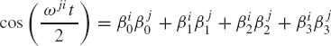
Example 8.3
As an example of the use of the quaternion algebra, we consider a rigid body whose orientation is defined at the initial configuration before displacement by the transformation matrix B expressed in terms of the four Euler parameters β0, β1, β2, and β3. In this example, we consider three cases of the body rotation with a constant angular velocity. The first is the rotation of the body about the global X axis, the second is the rotation of the body about the global Y axis, and the third is the rotation about the global Z axis. In the three cases, we assume that the axes of rotations are defined in the global system. For simplicity of notation, we drop the superscript that indicates the body number.
Rotation about the Global X Axis: If the body rotates with a constant angular velocity ω about the X axis, the final orientation of the body is defined by the transformation matrix C given by
where A is the transformation matrix resulting from the rotation of the body about the global X axis with a constant angular velocity. The order of the matrix multiplication used in the preceding equation is due to the fact that the axis of rotation is defined in the global system. It can be shown that the four Euler parameters that define the matrix A are as follows:
Using the quaternion multiplication role, it can be shown that the four Euler parameters γ0, γ1, γ2, and γ3 that define the transformation matrix C are given by
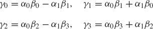
Rotation about the Global Y Axis: In the case of the rotation with a constant angular velocity about the Y axis, the four Euler parameters that define the matrix A are given by
The four Euler parameters that define the matrix C are then given by
Rotation about the Global Z Axis: If the rotation is about the global Z axis, the four Euler parameters that define the matrix A are given by
In this case, the four Euler parameters of the matrix C that defines the final orientation of the body are as follows:
The nonimpulsive contact between rigid bodies does not result in instantaneous change in the system velocities and momentum. Examples of this type of nonimpulsive contact are cam and follower contact, wheel and rail contact, disk rolling on a flat surface, and nonimpulsive contact between the end effector of a robot and a surface, among others. In this section, the kinematic equations that describe the nonimpulsive contact between two surfaces of two rigid bodies in the multibody system are formulated in terms of the system generalized coordinates and the surface parameters. Each contact surface is defined using two independent parameters that completely define the tangent and normal vectors at an arbitrary point on the body surface. The surface parameters can be considered as a set of nongeneralized coordinates since there are no inertia or external forces associated with them (Shabana and Sany, 2001). In the contact model discussed in this section, the location of the contact points on the two surfaces is determined by solving the nonlinear differential and algebraic equations of the constrained multibody system. The equations of motion of the bodies in contact are developed using the principle of mechanics, and the contact constraint equations are adjoined to the system dynamic equations using the technique of Lagrange multipliers. Lagrange multipliers associated with the contact constraints are used to determine the generalized contact constraint forces.
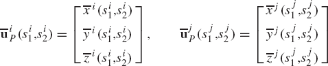
The two bodies in contact are denoted as bodies i and j. Contact between the two surfaces of the bodies is assumed to occur at point P. Two coordinate systems XiYiZi and XjYjZj are introduced for bodies i and j, respectively, as shown in Fig. 4. At a given instant of time, the location of the contact point P with respect to the coordinate systems of the two bodies is defined by the following two vectors:
The contact surface of body i is assumed to be defined by the two surface parameters si1 and si2, while the contact surface of body j is defined in terms of the surface parameters sj1 and sj2. Therefore, the local position vectors of the contact point, defined in Eq., 84 can be expressed in terms of the surface parameters as follows:
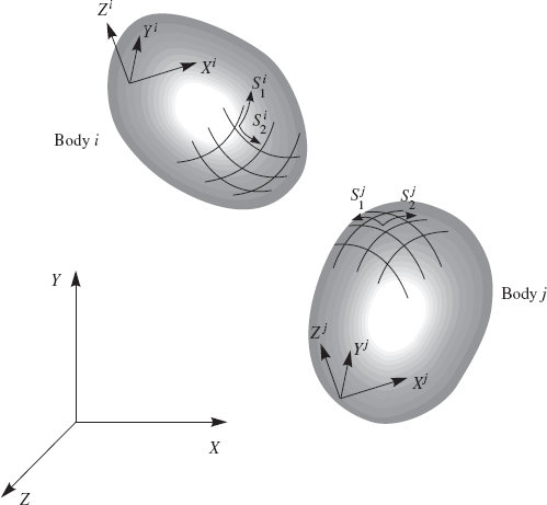
The tangents to the surface at the contact point on body i are defined in the body coordinate system by the following two independent, not necessarily orthogonal vectors:
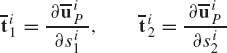
The normal to the surface at the contact point on body i is defined in the body coordinate system as
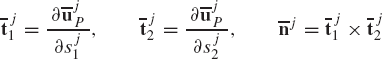
Similarly, the tangents and normal to the surface of body j at the contact point, defined in the body coordinate system, are given by
The tangent and normal vectors and their first and second derivatives with respect to the surface parameters are required to enforce the contact kinematic constraints discussed below.
In the multibody contact formulation presented in this section, it is assumed that the body motion is described using absolute Cartesian and orientation coordinates. For an arbitrary body k in the multibody system, the three-dimensional vector of absolute Cartesian coordinates Rk (k = i or j) is used to define the global location of the origin of the kth body coordinate system, while the orientation coordinates θk are used to define the orientation of the body coordinate system. Using this motion description, the global position vectors of the contact point on bodies i and j can be defined, respectively, as follows:
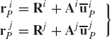
where Ai and Aj are the spatial transformation matrices that define the orientation of bodies i and j, respectively, in a global inertial frame of reference. These matrices are functions of the orientation coordinates θi and θj. Using this motion description, each unconstrained body has six independent coordinates. In the general case of contact where slipping is allowed, the contact conditions eliminate only one degree of freedom. Therefore, body i has five degrees of freedom with respect to body j.
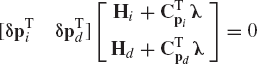
To formulate the contact conditions, five constraint equations expressed in terms of the generalized coordinates of the two bodies and the four surface parameters are introduced. These constraint equations impose the following two conditions (Roberson and Schwertassek, 1988; Litvin, 1994):
Two points on the two contact surfaces coincide. This implies that the global position coordinates of the contact point P evaluated using the generalized coordinates of body i are the same as the coordinates of the same point evaluated using the generalized coordinates of body j. This condition can be expressed mathematically as follows:
where the two vectors in this equation are defined explicitly in Eq. 89.
The normals to the two surfaces at the point of contact are parallel. This condition can be stated mathematically as follows:
where α is a constant and ni and nj are the normals at the contact point defined in the global coordinate system, that is,
It is important to point out that Eq. 91 leads to two independent equations only. An alternative to Eq. 91 is to use the unit normals instead of introducing the constant α. Another alternative to Eq. 91 is to use the tangent vectors to write two independent constraint equations which guarantee that the normals to the two surfaces remain parallel. These equations can be written as follows:
where
Equations 90 and 91 or, alternatively, Eqs. 90 and 93, represent five independent nonlinear equations which can be used to impose the contact conditions. Note that the normal and tangent vectors in Eq. 94 are expressed in terms of the first derivatives of the local coordinates of the contact point with respect to the surface parameters. Imposing the constraints of Eq. 93 at the acceleration level requires the evaluation of the third partial derivatives of the contact point coordinates with respect to the surface parameters. Note also that the five independent contact constraint equations can be used to identify five dependent variables (including the four surface parameters si1, si2, sj1, and sj2). Therefore, the surface parameters and one generalized coordinate can be eliminated using a coordinate partitioning scheme and the embedding technique as discussed previously in this book. In the remainder of this section, however, an alternative technique based on the augmented formulation that employs Lagrange multipliers is discussed.
The contact constraint formulation presented in the preceding section can be implemented in general-purpose multibody system algorithms. Recall that these contact constraints are formulated in terms of a mixed set of generalized and nongeneralized surface parameters. Using the principle of virtual work, the following Lagrange-D'Alembert form can be obtained:
where M is the system mass matrix, q is the vector of the system generalized coordinates, and Q is the vector of all forces acting on the system, excluding the constraint forces, which are eliminated automatically using the virtual work principle. The generalized force vector Q includes externally applied forces, gravity forces, and spring, damper, and actuator forces as well as friction forces. The constraint equations that describe mechanical joints and specified motion trajectories as well as the contact constraints can be written in the following form:
where s is the vector of the parameters that describe the geometry of the surfaces in contact. Virtual changes in the system coordinates and the surface parameters, which are consistent with the kinematic constraints, lead to
which for an arbitrary nonzero vector λ leads to
Adding Eqs. 95 and 98, one obtains
The procedure used to obtain the augmented formulation when only generalized coordinates are used (see Chapter 6) can be generalized for the case of system with nongeneralized coordinates. To demonstrate this, the preceding equation can be written as follows:
where
The vector p, which includes generalized coordinates and nongeneralized surface parameters, can be partitioned into two sets: the set of independent coordinates pi and the set of dependent coordinates pd, that is,
Each set, independent or dependent, may include nongeneralized surface parameters. According to this coordinate partitioning, Eq. 100 can be written as follows:
Assuming that the constraint sub-Jacobian Cpd associated with the dependent generalized and nongeneralized coordinates has a full row rank, the vector of Lagrange multipliers λ can be selected to be the solution of the following system of algebraic equations:
It follows from Eqs. 103 and 104 that
Since the element of the vector pi are assumed to be independent, Eq. 105 leads to
Combining Eqs. 104 and 106 and using the definition of H given by Eq. 101, one obtains
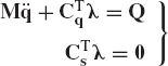
Differentiating the constraints of Eq. 96 twice with respect to time yields
where Qd is a vector that absorbs terms which are quadratic in the first time derivatives of the coordinates and the surface parameters. Combining Eqs. 107 and 108 yields (Shabana and Sany, 2001)

It is important to point out that the sub-Jacobian Cs associated with the surface parameters must have rank equal to the number of these surface parameters to be able to solve for the second derivatives of the coordinates and surface parameters as well as the vector of Lagrange multipliers. Therefore, the surface profiles must be chosen to guarantee a point contact. In the case of a line contact, such as in the case of a contact between a cylinder and a flat surface, there are infinite number of solutions, and the matrix Cs has a rank that is not equal to the number of the surface parameters. This special case can also be handled using the algorithm proposed in this chapter by changing the number of equations and variables required to describe the contact.
The case of a point contact is described using five independent constraint equations and four independent surface parameters. Nonetheless, the second equation of Eq. 107 implies that for each contact, there is only one nontrivial solution since the rank of the matrix CsT is four times the number of contacts. Therefore, there is only one independent Lagrange multiplier associated with each contact. That is, there is only one independent generalized contact force, which can easily be visualized in simple contact configurations to be the normal force at the point of contact. The nonconformal kinematic conditions defined by Eqs. 90 and 93 do not allow separation or penetration of the two contact surfaces. These conditions when used in multibody system algorithms must be satisfied at the position, velocity, and acceleration levels. Another alternative for using the constraint contact formulation is to use an elastic contact method that employs a compliant force model to describe the interaction between the two contact surfaces. This elastic force model, which can be defined in terms of the penetration and stiffness and damping coefficients, can be introduced to the dynamic equations of motion using generalized applied forces instead of kinematic constraints. When elastic contact methods are used, separation and penetration of the two surfaces in the small contact region are allowed. Therefore, the elastic contact method does not lead to elimination of degrees of freedom as in the case of the constraint contact formulation (Khulief and Shabana, 1987; Shabana et al., 2008).
The equations of motion that govern the dynamics of multibody systems are highly nonlinear as the results of the finite rotations and the nonlinear kinematic constraints imposed on the motion of the bodies. One method that can be used to study the stability of constrained multibody systems is to perform the time domain dynamic simulations and examine the stability of the system using numerical results obtained from the simulation. In addition to the time domain simulations that do not involve linearization of the dynamic equations, another method that can also be used is to linearize the nonlinear dynamic equations at certain configurations (points in time) and obtain the eigen solution that can be used to shed light on the system stability. For a multi-degree-of-freedom system with velocity dependent forces, as it is the case in many multibody system applications; the eigenvalues can be real and/or complex conjugates. As it is known from the theory of vibration, any eigenvalue with a positive real part leads to unstable solution, zero real parts lead to what is known as critically stable solutions, whereas negative real parts lead to stable solutions. Because the complete solution of a linear system can be written as a linear combination of mode shapes associated with the eigenvalues, the system becomes unstable if any of the eigenvalues has a positive real part. In order to obtain the eigenvalue solution, the constraint forces and dependent coordinates are eliminated using the embedding technique as discussed in Chapter 6 of this book. In this case, one obtains the following system of equations of motion expressed in terms of the degrees of freedom:
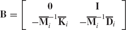
In this equation
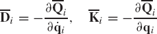
Using these two symmetric matrices and assuming that the mass matrix
This linearized system of equations has a number of equations nd equal to the number of the system degrees of freedom. All the matrices that appear in Eq. 112 are real and symmetric matrices.
The general purpose computer code SAMS/2000 described in Chapter 9 allows for solving two eigenvalue problems based on the system given by Eq. 112. In the first eigenvalue problem, the effect of the damping is neglected, that is,
In order to determine the system natural frequencies at selected points in time, the effect of the damping forces is neglected. In this case, Eq. 112 leads to
In order to determine the eigenvalues and eigenvectors, one assumes a solution in the form qi = Sest, where S is the vector of amplitudes and s is the frequency. Substituting this assumed solution into Eq. 113, one obtains
This equation defines a generalized eigenvalue problem. In order to have a nontrivial solution, one must have the following condition:
This determinant defines the characteristic equation which has nd roots, (S1)2, (S2)2,..., (Snd)2, called the eigenvalues. Associated with each root (sk)2, there is an eigenvector Sk, which can be determined to within an arbitrary constant using the following system of homogeneous equations:
Since the mass and stiffness matrices
In the case of general damping matrix, another procedure is used to determine the eigenvalues and eigenvectors of the multibody system. In this more general case, some of the eigenvalues and eigenvectors can be complex conjugates. Since the coordinates are real, a procedure for defining real mode shapes is described in this section. In the case of general damping forces, the linearized system of Eq. 112 is also used as the starting point. In the state space formulation, one can define the state vector
Note that the dimension of the vector z is 2 × nd. Using Eqs. 112 and 117, one can write the following system of equations:
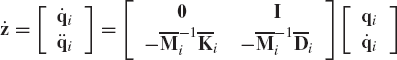
This equation can be written as
where
In order to determine the eigenvalues and eigenvectors of the matrix B of Eq. 119, a solution of the following form is assumed:
In this equation, the vector S has dimension 2 × nd, and s is a constant to be determined. Substituting Eq. 121 into Eq. 119, one obtains the following system of homogeneous equations:
This system of homogeneous equations has a nontrivial solution if and only if
This is the characteristic equation that has roots sk, k = 1, 2, ..., 2 × nd. These roots define the eigenvalues of the system of Eq. 122. Associated with each eigenvalue sk, there is an eigenvector Sk that can be determined to within an arbitrary constant using the following system of homogeneous equations:
In the case of multibody systems the roots sk of the characteristic equation can be real and/or complex. Complex roots will appear as pairs of complex conjugates, which can have negative, zero, or positive real parts. The imaginary parts define the frequency of oscillations, while the real parts define the system stability. Any eigenvalue with a positive real part will render the system unstable. For linear problems, the solution can be written as a linear combination of the eigenvectors (mode shapes). The part of the solution due to eigenvectors associated with eigenvalues, which have negative real parts converges to zero, and therefore, such eigenvectors do not render the system unstable. The linearized system of Eq. 112, therefore, can shed light on the behavior of the multibody system in the neighborhood of the time-point at which the linearization is made.
As previously mentioned, complex eigenvalues appear as complex conjugates. For example, if sk and sk+1 are two complex eigenvalues, they will take the following form:
where
Substituting Eq. 125 into Eq. 126 and rearranging the terms, one obtains
Euler's formula for complex variables can be used to write
Substituting this equation into Eq. 127, one obtains
Since z must be real, Sk and Sk+1 must appear as complex conjugate vectors. That is, i(Sk−Sk+1) in the preceding equation is a vector of real numbers. Using this fact, the real mode shapes associated with complex eigenvalues can be extracted using the eigenvectors obtained from the linearized multibody system equations of Eq. 122. It is important, however, to point out that such a linearized solution may not give in some applications accurate prediction of the stability of the multibody systems whose dynamics are, in general, governed by highly nonlinear differential equations.
In the case of lightly damped (under damped) modes, the eigenvalues are complex and take the form given in Eq. 125. Using the elementary theory of vibrations, one can write pk and ωk of Eq. 125 as
In this equation, ξk is recognized as the modal damping ratio, ωnk is the modal natural frequency of oscillation, and ωk as the modal damped frequency; all associated with mode k. The preceding two equations can be solved for ωnk and ξk as
Heavily damped modes are, in general, real and do not contribute to the oscillatory motion of the system.
Use the Rodriguez formula to prove the orthogonality of the rotation matrix.
Using the Rodriguez formula, show that the axis of rotation is an eigenvector of the spatial rotation matrix. Determine the associated eigenvalue.
Use the Rodriguez formula to determine the form of the spatial rotation matrix in the case of infinitesimal rotations.
Use the Rodriguez formula to show that two general consecutive three dimensional rotations are not commutative.
Discuss the singularity associated with Euler angles and show that this singularity problem does not arise when Euler parameters are used.
Use Newton-Euler equations to define the equations of motion of a rigid body in space in terms of Euler parameters.
Discuss the singularity problem associated with Rodriguez parameters.
Use Newton-Euler equations to define the equations of motion of a rigid body in space in terms of Rodriguez parameters.
Find the relationships between Euler and Rodriguez parameters.
The orientation of a rigid body is defined by the four Euler parameters
At the given orientation, the body has an instantaneous absolute angular velocity defined by the vector
Find the time derivatives of Euler parameters. Find also the time derivatives of Rodriguez parameters.
In the preceding problem, find the time derivatives of Euler angles.
Use the Rodriguez formula and unit vectors along the joint axes of rotation, defined in a fixed coordinate system, to obtain the transformation matrix that defines the orientation of body 4 shown in Fig. P1. Show that the form of this transformation matrix is the same as the Euler angle transformation matrix.
Discuss the use of the quaternions in describing the relative rotations between rigid bodies.
