In the kinematic analysis, we are concerned with studying motion without considering the forces that produce the motion. Unlike the case of dynamic analysis, where the motion of the system due to known forces is determined, the objective of the kinematic analysis is to determine the positions, velocities, and accelerations as the result of known prescribed input motions. Recall that the degrees of freedom of a mechanical system, by definition, are the smallest set of independent coordinates that are required to define the system configuration. If the degrees of freedom and their time derivatives are known, other coordinates and their time derivatives that represent the displacements, velocities, and accelerations of the bodies of the system can be expressed in terms of the system degrees of freedom and their time derivatives. This leads to the displacement, velocity, and acceleration kinematic relationships that can be solved for the state of the system regardless of the forces that produce the motion.
There are three stages that must be followed for the complete kinematic analysis of a mechanical system: position, velocity, and acceleration analyses. In the position analysis, the displacement kinematic relationships are solved assuming that the selected degrees of freedom of the system are specified. These relationships are, in general, nonlinear functions in the system coordinates and their solution may require the use of an iterative numerical procedure such as Newton-Raphson methods. The velocity and acceleration kinematic equations can be obtained by differentiating the displacement equations, once and twice, respectively. This procedure leads to a system of linear algebraic equations in the velocities and accelerations.
In this chapter, the constrained motion of systems that consist of interconnected bodies is examined. Two different, yet equivalent, approaches are presented in this chapter for the kinematic analysis of multibody systems whose degrees of freedom are specified. The first is the classical approach, which is suited for studying the kinematics of systems that consist of small numbers of bodies and joints. The use of this approach is demonstrated by several examples presented in this chapter. No detailed discussion of this approach is provided, since the focus of the book is on computational methods that can be used in the analysis of more complex systems. The second approach, on the other hand, can be used for solving large-scale applications, which consist of large numbers of bodies and joints. In this approach, the algebraic kinematic constraint relationships between coordinates are formulated and used to develop a number of equations equal to the number of unknown coordinates. These constraint equations, which are, in general, nonlinear functions of the coordinates, can be solved using iterative numerical and computer methods to determine the positions of the bodies in the system. By differentiating the constraint equations once, and twice with respect to time, linear systems of equations in the velocities and accelerations can be obtained. These linear equations can be solved in a straightforward manner to determine the first and second time derivatives of the coordinates. Computer implementation of this general computational procedure is discussed and several examples are presented in order to demonstrate its use.
Throughout the analysis presented in this chapter and the following chapters, it is assumed that the multibody systems consist of rigid bodies, such that the effect of the body deformation can be neglected. In the rigid body analysis, it is assumed that the distance between two arbitrary points on the body remains unchanged. The assumption of rigidity is justified when the components of the multibody system are made of bulky solids that experience only small deformations such that the effect of this deformation on the overall motion is negligible. If the interest, however, is to determine the stresses, or if the deformations of the bodies are large such that their effect cannot be neglected, the rigid body assumption is no longer adequate and a deformable body modeling approach must be adopted. In this section, the kinematic equations that describe the general planar motion of a rigid body are developed in terms of the body coordinates. The transformation matrix that defines the orientation of the body is derived and is used to develop the position equations that describe an arbitrary displacement of the rigid body.
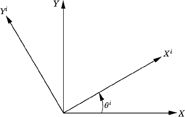
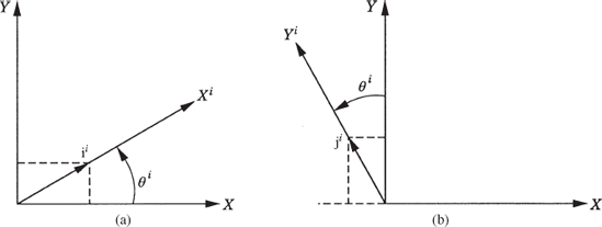
We consider the problem of a simple finite rotation about a fixed axis and develop the relationships between the axes of different coordinate systems as the result of the finite rotation. These relationships define the coordinate transformation between moving coordinate systems. Figure 1 shows two coordinate systems XY and XiYi. The axis Xi is assumed to make an angle θi with respect to the X axis of the coordinate system XY. We assume for the moment that the origins of both coordinate systems coincide. Let i and j be unit vectors along the X and Y axes, respectively, and Let ii and ji be, respectively, unit vectors along the Xi and Yi axes. Using Fig. 2a, the components of the unit vector ii can be expressed in the XY coordinate system as
From Fig. 2b, one can also show that the components of the unit vector ji can be expressed in the coordinate system XY as
Equations 1 and 2 define the unit vectors along the axes of the coordinate system XiYi in terms of unit vectors along the axes of the coordinate system XY. To obtain the inverse relationship, we multiply Eqs. 1 and 2 by cos θi and sin θi, respectively, and subtract the resulting equations. This leads to
Using the trigonometric identity (cos θi)2 + (sin θi)2 =1, the equation above leads to
This equation defines a unit vector along the X axis in terms of the unit vectors along the axes of the XiYi coordinate system. Similarly, multiplying Eqs. 1 and 2 by sin θi and cos θi, respectively, and adding leads to
in which the unit vector j along the Y axis is expressed in terms of the unit vectors ii and ji of the coordinate system XiYi.
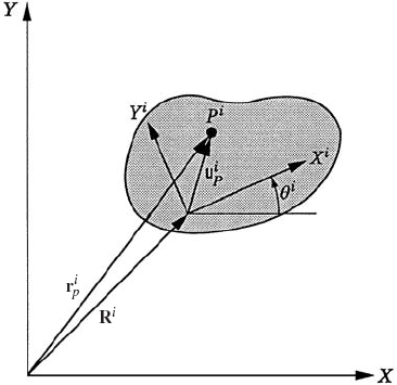
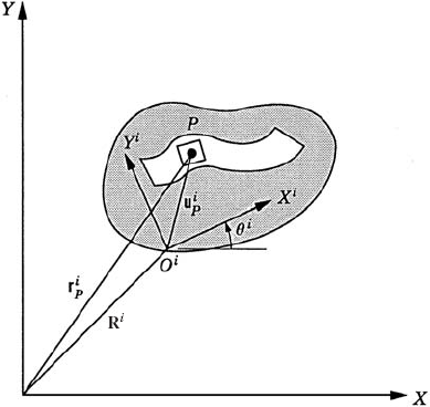
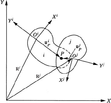
For the convenience of describing the motion of the rigid bodies in the multibody system, we assign a coordinate system for each body. The origin of this body coordinate system is rigidly attached to a point on the body, and therefore, the coordinate system experiences the same rigid body motion as the body. Let XiYi, as shown in Fig. 3, be the body coordinate system and XY be a selected global inertial frame of reference that is fixed in time. Let Pi be an arbitrary material point on the body. The coordinates of point Pi in the body coordinate system are fixed and can be defined by the vector
which can also be written in terms of unit vectors along the axes of the coordinate system XiYi as
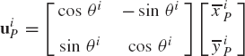
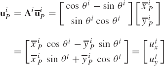
where ii and ji are, respectively, unit vectors along the Xi and Yi axes of the body coordinate system. Substituting Eqs. 1 and 2 into Eq. 7 yields the coordinates of the vector
where uiP is the global representation of the vector
This equation can also be written in the following form:
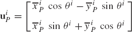
or in the following matrix form:
Using Eq. 6, Eq. 11 can be written simply as
where
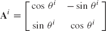
The matrix Ai is an orthogonal matrix because
where I is the 2 × 2 identity matrix.
The global position vector of the arbitrary point Pi in the fixed XY coordinate system can be written as shown in Fig. 3 as the sum of the two vectors Ri and uiP, where Ri is the global position vector of the origin Oi of the coordinate system XiYi. One can then write the following equation:
which upon the use of Eq. 12 yields
It is clear from Eq. 16 that the global position vector of an arbitrary point on the rigid body i can be written in terms of the rotational coordinate of the body θi, as well as the translation of the origin of the body reference Ri. That is, the most general rigid body displacement can be described by a translation of a reference point plus a rotation about an axis passing through this point.
The second step in the kinematic analysis is to determine the velocities of the bodies in the system. In the velocity analysis, it is assumed that the positions and orientations of the bodies are already known from the position analysis. The absolute velocity of a point on a rigid body that undergoes planar motion can be obtained by differentiating Eq. 16 with respect to time. This yields
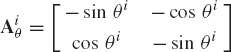
By using Eq. 13, the time derivative of the transformation matrix can be written as
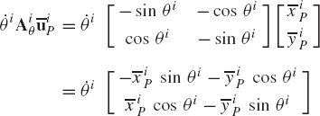
where Aiθ is the partial derivative of the rotation matrix with respect to the rotational coordinate θi and is given by
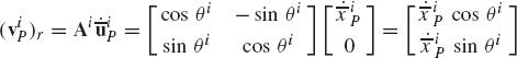
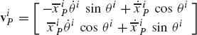
The velocity vector of the arbitrary point Pi can then be expressed as
This equation defines the absolute velocity vector of point Pi in terms of the derivatives of the coordinates Ri and θi of the rigid body.
The second term on the right-hand side of Eq. 20 can be written explicitly as
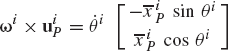
Equation 21 can be written in a simple form if we define the angular velocity vector ωi of body i as
where k is a unit vector along the axis of rotation that is perpendicular to the plane of the motion. Equation 22 can also be written in an alternative form as
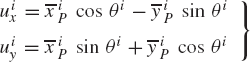
The velocity vector of an arbitrary point on the rigid body can be expressed in terms of the angular velocity vector. To demonstrate this, we evaluate the vector ωi × uip where the vector uiP is given by Eq. 12 as
where uix and uiy are the components of the vector uiP given by
It follows that
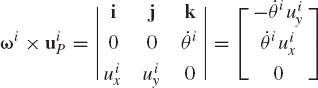
which upon using the definition of the components uix and uiy of Eq. 25 leads to
Comparing Eqs. 27 and 21 and using Eqs. 18 and 24, we obtain the following identity:
Using this identity, the absolute velocity vector of an arbitrary point on the rigid body i can be written in terms of the angular velocity vector as
which indicates that the velocity of any point Pi on the rigid body can be written in terms of the velocity of a reference point Oi plus the relative velocity between the two points. That is
where viP and viO are, respectively, the absolute velocities of points Pi and Oi, and viPO is the relative velocity of point Pi with respect to point Oi and is given by
It will be shown in Chapter 7 that equations similar to Eqs. 29-31 can still be used in the case of the spatial motion of rigid bodies. In the more general case of spatial motion, the transformation matrix Ai and the angular velocity vector ωi take forms different from those used in the planar analysis.
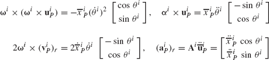
The absolute acceleration of a point fixed on a rigid body can be obtained by differentiating the velocity equation with respect to time. If Eq. 20 is differentiated with respect to time, one obtains the acceleration of an arbitrary point Pi on the rigid body i as
where
which upon substitution into Eq. 32 leads to
It can be shown that
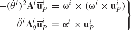
where ωi is the angular velocity vector, and αi is the angular acceleration vector of body i defined as
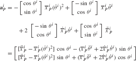
By substituting Eq. 35 into Eq. 34, one obtains
which can be rewritten as
where
The normal component has a magnitude
Equation 38 can also be written as
where aiPO is the relative acceleration of point Pi with respect to point Oi and is defined as
The forms of the acceleration equations, given by Eqs. 37-41, can still be used in the case of the spatial motion of rigid bodies as will be demonstrated in Chapter 7.
In the preceding sections, the kinematic equations that define the position, velocity, and acceleration of an arbitrary point fixed on a rigid body were developed. In this section, we present the kinematic equations of a point moving on a rigid body. Figure 4 shows a particle
point P moving on a rigid body i. The position vector of point P with respect to the body coordinate system XiYi is defined by the vector
where Ri is the global position vector of the reference point, and Ai is the transformation matrix from the body coordinate system to the global coordinate system. The vector
The absolute velocity of point P can be obtained by differentiating Eq. 42 with respect to time. This leads to

By using the identity of Eq. 28, Eq. 43 takes the form
where
Equation 44 can also be written as
where
The absolute acceleration of point P can be obtained by differentiating Eq. 46 or, equivalently, Eq. 43 with respect to time. This leads to
The second and third terms on the right-hand side of Eq. 47 are, respectively, the normal and tangential components of the acceleration defined in the preceding section by Eq. 35. Combining the fourth and fifth terms in the right-hand side of Eq. 47, this equation reduces to
where αi is the angular acceleration vector of the coordinate system of body i and uiP is as defined by Eq. 24. Using Eq. 45 and an identity similar to Eq. 28, one can show that
Substituting Eq. 49 into Eq. 48, one obtains
where
in which (aiP)r is the relative acceleration of point P with respect to the coordinate system of body i.
The fourth term in the right-hand side of Eq. 50 given by
is called the Coriolis component of the acceleration. This component of the acceleration has a direction along a line perpendicular to both ωi and (viP)r. In the special case where point P is fixed, the vectors (aiP)r and (aiP)c are identically the zero vectors and Eq. 50 reduces, in this special case, to the equation that defines the acceleration of a point fixed on the rigid body.
Mechanical systems are assemblages of bodies connected by joints. The purpose of the joints is to transmit the motion from one body to another in a certain fashion. In this section, we briefly discuss the formulation of some of the joint constraints and introduce the mobility criterion that can be used to determine the number of degrees of freedom of a multibody system. A more detailed formulation of the planar joints in terms of the system coordinates is presented in Section 9 of this chapter, while a more detailed analysis of the spatial joints is presented in Chapter 7.
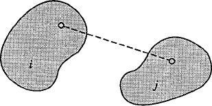
The kinematic relationships that describe the joint constraints can be formulated using a set of algebraic equations. As will be seen in the remainder of this book, the form of these equations depends on the parameters or coordinates used to describe the motion of the system. Figure 5a shows two bodies, i and j, in planar motion, which are connected by a revolute joint. The joint definition point is defined by point P. The corresponding point on body i is denoted as Pi while the corresponding point on body j is denoted as Pj. The conditions for the revolute joint require that point Pi on body i remains in contact with point Pj on body j throughout the motion. This condition can be expressed mathematically as
where riP is the global position vector of point Pi, while rjP is the global position vector of point Pj. The conditions given by Eq. 53 eliminate the possibility of the relative translation between the two bodies. The two bodies, however, have the freedom to rotate with respect to each other. This is the only relative motion between the two bodies that can occur as the result of their connectivity using the revolute joint. Therefore, the revolute joint in the planar analysis has one degree of freedom since it eliminates two degrees of freedom of the relative translation between the two bodies along two perpendicular axes.
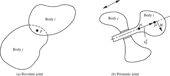
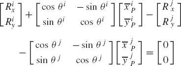
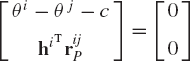
Another one-degree-of-freedom joint in the planar kinematics is the translational (prismatic) joint shown in Fig. 5b. In this case, the only relative motion between the two bodies i and j is the relative translation along the joint axis. In the case of the prismatic joint, there are two kinematic constraint conditions that restrict two possible relative displacements. First, there should be no relative rotation between the two bodies. Second, there is no relative translation between the two bodies along an axis perpendicular to the axis of the prismatic joint. These two conditions can be stated mathematically as
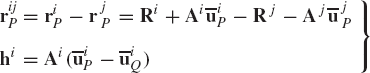
where θi and θj are, respectively, the angular orientations of bodies i and j, c is a constant, rijP is a vector that connects the two points Pi and Pj defined, respectively, on bodies i and j on the joint axis, and hi is a vector defined on body i perpendicular to the joint axis.
While more detailed analysis of the spatial joints will be presented in Chapter 7, as previously mentioned; in this section, a brief discussion on the formulation of the spatial joint constraints is presented in order to better understand the formulation of the mobility criteria used in this chapter. In the spatial kinematics, the unconstrained motion of a rigid body is described using six independent coordinates or degrees of freedom. Three of these degrees of freedom represent the translations of the body along three perpendicular axes and three degrees of freedom represent three independent rotational displacements. Figure 6 shows examples of mechanical joints in spatial kinematics. The spherical joint shown in Fig. 6a allows only three relative rotational motions between the two bodies i and j connected by this joint. In this case, there is no relative translation between the two bodies, and hence, one needs three kinematic constraint conditions that eliminate the freedom of the two bodies to translate with respect to each other. Let point P be the joint definition point, Pi be the corresponding point on body i, and Pj be the corresponding point on body j. The three kinematic conditions for the spherical joint require that points Pi and Pj remain in contact throughout the motion. These kinematic conditions can be stated in a vector form as
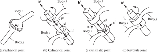
where riP and rjP are three-dimensional vectors that represent, respectively, the global position vectors of points Pi and Pj. The spherical joint is considered as a three-degree-of-freedom joint, because the three kinematic constraints of Eq. 55 do not impose any restriction on the relative rotations between the two bodies.
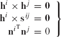
Figure 6b shows the two-degree-of-freedom cylindrical joint that allows relative translational and rotational displacements between bodies i and j along the joint axis. Two components of the relative translational displacements and two components of the relative rotational displacements along two axes perpendicular to the joint axis are not allowed. In order to eliminate four degrees of freedom, four kinematic constraint conditions are imposed in the case of a cylindrical joint. Let hi be a vector drawn on body i along the joint axis, and hj be a vector drawn on body j along the joint axis. Also, let sij be a vector of variable magnitude that connects points Pi and Pj on bodies i and j, respectively. The vector sij is defined on the axis of the cylindrical joint as shown in Fig. 6b. Throughout the motion of the bodies i and j that are connected by the cylindrical joint, the vector hi must remain collinear to the vectors hj and sij. The kinematic constraint conditions of the cylindrical joint can then be written as
As explained in Chapter 2, each vector equation in Eq. 56 contains only two independent equations, that is, the number of the independent kinematic constraint equations is four, leaving two degrees of freedom for the cylindrical joint.
The case of the prismatic joint in the spatial kinematics can be obtained as a special case from the case of the cylindrical joint in which the relative rotation between the two bodies i and j is not allowed. In order to mathematically define this condition, two orthogonal vectors ni and nj are drawn perpendicular to the joint axis on bodies i and j, respectively, as shown in Fig. 6c. To eliminate the freedom of the rotations between the two bodies i and j, the vectors ni and nj must remain perpendicular throughout the motion. By considering the prismatic joint as a special case of the cylindrical joint, one needs to add one condition in Eq. 56, leading to the following kinematic constraint equations for the prismatic joint:
where hi, hj, and sij are as defined in Eq. 56. Equation 57 contains five independent constraint equations that define the kinematic conditions for the single-degree-of-freedom prismatic joint in the spatial analysis.
Similarly, the revolute joint shown in Fig. 3-6d can be considered a special case of the cylindrical joint where the relative translation between the two bodies is not allowed. The revolute joint in the spatial kinematics is a one-degree-of-freedom joint. In addition to the constraint equations of the cylindrical joint, one needs another condition that guarantees that the distance between the two points Pi on body i and Pj on body j, defined on the joint axis, remains constant throughout the motion. If sij (Fig. 6b) is the vector that connects points Pi and Pj, the kinematic conditions for the revolute joint obtained as a special case of the cylindrical joint are given by
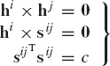
where the vectors hi, hj, and sij are the same as in the case of the cylindrical joint and c is a constant. The last equation of Eq. 58 guarantees that the length of the vector sij remains constant throughout the motion.
The universal (Hooke) joint shown in Fig. 7a is a two-degree-of-freedom joint since it allows relative rotation between the bodies connected by this joint about two perpendicular axes. The constraint equations for this joint can be obtained as a special case of the spherical joint. The four conditions for the universal joint can be written as
where riP and rjP are the global position vectors of point Pi on body i and point Pj on body j that coincide with point P at the intersection of the two bars of the cross, and the vectors hi and hj are two vectors defined on body i and body j, respectively, along the bars of the cross as shown in Fig. 7a.
The screw joint shown in Fig. 7b can be considered a special case of the cylindrical joint in which the translation and rotation along the joint axis are not independent. They are related by the pitch of the screw. By considering the screw joint as special case of the cylindrical joint, the constraint equations of this joint can be defined using the
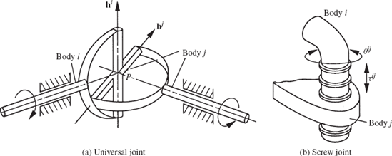
relationships
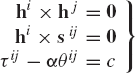
where hi, hj, and sij are as defined in the case of the cylindrical joint, τij is the relative translation, θij is the relative rotation, α is the pitch rate of the screw joint, and c is a constant that accounts for the initial relative displacements between the two bodies.
It was shown in this section that the number of independent kinematic conditions of a joint is equal to the number of degrees of freedom eliminated as the result of using this joint. One of the basic steps in the kinematic and dynamic analysis of mechanical systems is to determine the number of the system degrees of freedom or the independent coordinates required to determine the configuration of the system. There are different types of multibody systems that consist of different numbers of bodies interconnected by different numbers and types of joints. The degrees of freedom of the system define the minimum number of independent inputs required to drive or control the system. A multibody system with zero degrees of freedom is a structure. The components of such a system are not permitted to undergo relative rigid body motion regardless of the forces acting on the system. Most mechanisms that are in use in industrial and technological applications are designed as single-degree-of-freedom systems. Their motion is controlled by a single input that is transmitted to a single output. Robotic manipulators, on the other hand, are multidegree-of-freedom systems. They require several inputs in order to drive the manipulator and control the position of its end effector. In this section, a simple criterion is presented for determining the number of degrees of freedom of multibody systems.
As pointed out previously, the configuration of a rigid body that undergoes unconstrained planar motion can be identified using three independent coordinates or degrees of freedom. These coordinates describe the translational motion of the body along two perpendicular axes as well as the rotation of the body. A planar system that consists of nb unconstrained bodies has 3 × nb coordinates. If these bodies are connected by joints, the number of the system degrees of freedom decreases. The reduction in the system degrees of freedom depends on the number of independent constraint equations that describe the joints. In planar motion, the number of the system degrees of freedom can be evaluated according to the mobility criterion
where nd is the number of the system degrees of freedom, nb is the number of the bodies in the system, and nc is the total number of linearly independent constraint equations that describe the joints in the system. Each revolute or prismatic joint in the planar analysis introduces two kinematic constraints that reduce the number of degrees of freedom by two.
Example 3.1
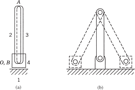
The slider crank mechanism shown in Fig. 8 consists of four bodies, the ground (fixed link) denoted as body 1, the crankshaft denoted as body 2, the connecting rod denoted as body 3, and the slider block denoted as body 4. The system has three revolute joints at O, A, and B, each introduces two kinematic constraint equations that make the total number of kinematic constraints of the revolute joints six. The system has one prismatic joint between the slider block and the fixed link. This joint introduces two kinematic relationships. The fixed link constraints (ground constraints) are three since in planar motion two conditions are required to eliminate the freedom of the body to translate and one condition is required to eliminate the freedom of the body to rotate. The total number of constraints nc is
Thus, the use of Eq. 61 leads to
That is, the mechanism has only one degree of freedom.
In spatial kinematics, the configuration of a rigid body in space is identified using six coordinates. If the mechanical system consists of nb bodies, the mobility criterion in the spatial analysis can be written as
The freedom of the relative translation between two bodies is eliminated if they are connected by a spherical joint. It follows that a spherical joint reduces the number of the system degrees of freedom by three. A cylindrical or a universal joint introduces four independent kinematic constraint equations that reduce the number of degrees of freedom by four. A revolute, prismatic, or a screw joint, on the other hand, introduces five kinematic constraint conditions that reduce the number of degrees of freedom by five.
Example 3.2
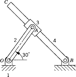
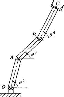
The spatial RSSR (revolute, spherical, spherical, revolute) mechanism shown in Fig. 3-9 consists of four bodies. Body 2 is connected to body 1 at O by a revolute joint, body 3 is connected to body 2 at A by a spherical joint, body 4 is connected to body 3 at B by a spherical joint, and body 4 is connected to body 1 at C by a revolute joint. Since each spherical joint introduces three kinematic constraints, the spherical joints at A and B introduce six kinematic constraint conditions. The two revolute joints at O and C introduce 10 constraints. In the spatial analysis, six conditions are required to eliminate the freedom of the body to translate or rotate. Thus, the number of fixed link constraints (ground constraints) for body 1 is six. The total number of constraint equations for the RSSR mechanism is
Using the mobility criterion of Eq. 64, the number of system degrees of freedom can be determined as
which indicates that the system has two degrees of freedom. One of these degrees of freedom is the freedom of the coupler link (body 3) to rotate about its own axis.

In this section, the classical approach used for the kinematic analysis is briefly discussed. This intuitive approach, which can be used in the analysis of systems that consist of a small number of interconnected bodies, is not suited for the study of the kinematics of complex systems. In the classical approach, analytical or graphical methods can be used. If the degrees of freedom of the system are specified, one can obtain small number of equations that can be solved numerically or using graphical techniques. The use of the analytical kinematic equations will be demonstrated in this section using several examples.
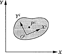
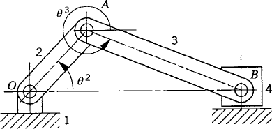
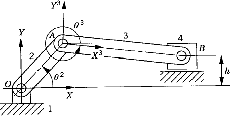
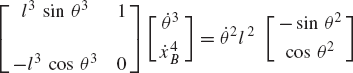
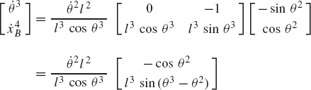
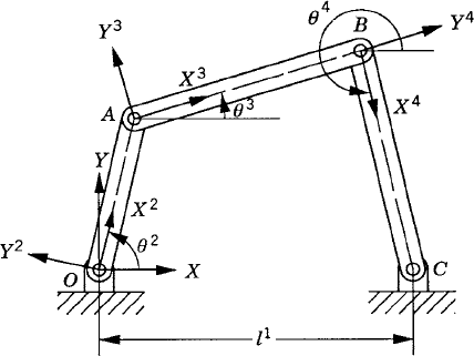
In order to demonstrate the use of the graphical techniques first, we consider the slider crank mechanism shown in Fig. 10. If the dimensions of the mechanism links are given and if the rotation of the crankshaft is specified, one can use nonlinear trigonometric functions to determine the positions and orientations of all other bodies in the mechanism. This step of the kinematic analysis constitutes the step of the position analysis, and it is considered as the most difficult step in the classical approach since one has to deal with nonlinear algebraic equations that involve trigonometric functions. For example, if the crank angle θ2 is given, one can write the following position equations for the slider crank mechanism shown in Fig. 10:
In these equations, l2 and l3 are the lengths of the crankshaft and connecting rod, respectively; θ3 and x4B are the angular orientation of the connecting rod and the position of the slider block, respectively; and h is the mechanism offset. Because the mechanism has one degree of freedom, which is considered in this example to be the angular position of the crankshaft, given the crankshaft angle θ2, the preceding two equations can be solved for the connecting rod angle θ3 and the slider block position x4B. For instance, the second equation of Eq. 67 can be solved for θ3. This value of θ3 can be substituted into the first equation to determine x4B. Alternatively, since θ2, l2, and l3 are known, one can draw a line diagram that represents the mechanism and from this diagram measure directly θ3 and x4B.
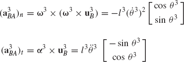
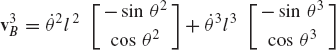
In general, the velocity and acceleration kinematic analyses are more straightforward as compared to the position analysis since the velocity and acceleration kinematic analyses involve linear equations only, while the kinematic position equations are, in general, nonlinear. For example, the absolute velocity of point B on the connecting rod can be written as shown in Eq. 64 as
If the angular velocity
Given the angular acceleration of the crankshaft, and knowing the mechanism coordinates from the position analysis and the mechanism velocities from the velocity analysis; one can use a procedure similar to the one used for the velocity diagram to draw the acceleration diagram that can be used to determine the angular acceleration
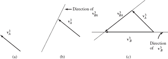
It is clear from the analysis presented in this section that the velocity diagram cannot be constructed before the step of the position analysis is completed. It is also clear that the acceleration diagram cannot be constructed before completing the position and velocity analysis steps since the acceleration analysis requires knowing the coordinates and velocities. This order of analysis must be followed regardless of the approach (graphical, analytical, or computational) used. It is also clear that once the nonlinear position equations are solved, the velocity and acceleration diagrams can be constructed in a straightforward manner since the velocity and acceleration equations are linear, as previously mentioned.
Another alternative to the use of the graphical solution in the classical kinematic approach is to obtain a small number of analytical equations for the mechanism. These analytical equations can be solved for the same unknown variables that can be determined using the graphical technique. The use of the analytical methods of the classical kinematic approach is demonstrated in this section using several examples.
Example 3.3
Figure 10 shows an offset slider crank mechanism that consists of four bodies. Body 1 is the fixed link or the ground, body 2 is the crankshaft, body 3 is the connecting rod, and body 4 is the slider block at B. The system has one degree of freedom, which is selected to be the angular orientation of the crankshaft θ2. Express the angular orientation of the connecting rod and the location of the slider block in terms of the degree of freedom. Also determine the angular velocity and acceleration of the connecting rod and the velocity and acceleration of the slider block in terms of the angular velocity
Solution. Consider point A to be the reference point of the connecting rod, the position vector of point B on the connecting rod can be written as
where R3 is the global position vector of the reference point A, A3 is the transformation matrix from the connecting rod coordinate system to the global coordinate system, and
and
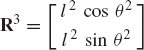
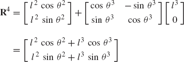
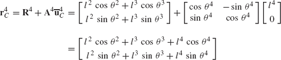
where θ2 and θ3 are, respectively, the angular orientations of the crankshaft and the connecting rod, and l2 and l3 are, respectively, the lengths of the crankshaft and the connecting rod. One can write the global position vector of point B as
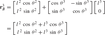
From the geometry of the slider crank mechanism, it is clear that

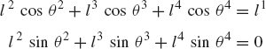
where x4B is the coordinate of the slider block in the horizontal direction and h is the magnitude of the offset. The preceding two equations lead to the following two scalar equations:
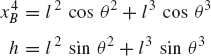
which imply that
and
By using Eq. 30, the velocity of point A on the crankshaft can be written using point O as the reference point as
Since O is a fixed point, v2O=0. Using Eqs. 27 and 31, the global velocity vector of point A is
The velocity of point B on the connecting rod can also be written as
Clearly, v2A = v3A since both represent the global velocity vector of the same point A. Using this fact and Eq. 27, the velocity of point B is given by
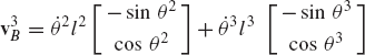
The slider block at B moves only in the horizontal direction, and as a consequence
The last two vector equations lead to
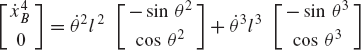
which can be rearranged and written as
or
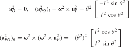
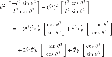
The acceleration equations can be obtained by differentiating the preceding equation or by using the general expression of Eq. 40. Using Eq. 40, the acceleration of point A on the crankshaft is
Since O is a fixed point, one has a2O = 0, and accordingly,
where
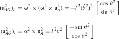
Thus
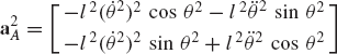
The acceleration of point B on the connecting rod is
Since a3A = a2A because A represents the same point on the crankshaft and the connecting rod, one has
where
Using the expression for a2A, one has
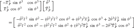
Since the slider block moves only in the horizontal direction, one has
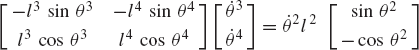
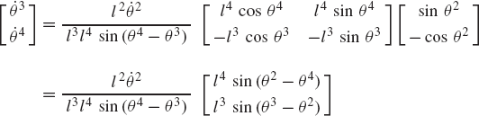
The preceding two vector equations lead to the following two scalar equations:
Since θ3 and
where
The kinematic equations obtained in this example can be programmed on a digital computer to obtain the values of the coordinates, velocities, and accelerations of the mechanism links for different values of θ2,
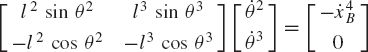
In some applications, the motion simulation of the single- and multidegree-of-freedom systems does not proceed smoothly with time. A lockup configuration may be encountered or more than one possible motion at certain mechanism configurations can occur. These cases are called singular configurations. The singularity of motion may depend on the nature of the driving input. For example, consider the slider crank mechanism shown in Fig. 12. First assume that the mechanism is driven by rotating the crankshaft with a given angular velocity
where l2 and l3 are, respectively, the lengths of the crankshaft and the connecting rod and θ2 and θ3 are, respectively, the angular orientations of the crankshaft and the connecting rod. Equation 65 can be used to define
Consider now the special case where l2 = l3 and θ2 = π/2; in this special case, one has l2 sin θ2 + l3 sin θ3 = 0, or sin θ2 + sin θ3 = 0. It follows that θ3 = 3π/2. In this configuration, cos θ3 = 0 and the coefficient matrix in Eq. 65 is singular. This implies that at this configuration, more than one possible motion can occur. One possible motion is that the crankshaft and the connecting rod are locked together and rotate as a single pendulum, as shown in Fig. 13a. Another possible motion is that the slider block moves to the right or to the left in the horizontal direction, as shown in Fig. 13b.
Table 3.1. Slider Crank Mechanism
θ2 | θ3 | |||||
|---|---|---|---|---|---|---|
0.000E + 00 | 0.000E + 00 | 0.600E + 00 | −0.250E + 02 | −0.000E + 00 | 0.000E + 00 | −0.750E + 03 |
0.200E + 00 | −0.995E − 01 | 0.594E + 00 | −0.246E + 02 | −0.297E + 01 | 0.189E + 03 | −0.724E + 03 |
0.400E + 00 | −0.196E + 00 | 0.577E + 00 | −0.235E + 02 | −0.572E + 01 | 0.387E + 03 | −0.647E + 03 |
0.600E + 00 | −0.286E + 00 | 0.549E + 00 | −0.215E + 02 | −0.808E + 01 | 0.600E + 03 | −0.522E + 03 |
0.800E + 00 | −0.367E + 00 | 0.513E + 00 | −0.187E + 02 | −0.985E + 01 | 0.827E + 03 | −0.360E + 03 |
0.100E + 01 | −0.434E + 00 | 0.471E + 00 | −0.149E + 02 | −0.109E + 02 | 0.106E + 04 | −0.173E + 03 |
0.120E + 01 | −0.485E + 00 | 0.426E + 00 | −0.102E + 02 | −0.112E + 02 | 0.126E + 04 | 0.169E + 03 |
0.140E + 01 | −0.515E + 00 | 0.382E + 00 | −0.488E + 01 | −0.108E + 02 | 0.140E + 04 | 0.183E + 03 |
0.160E + 01 | −0.523E + 00 | 0.341E + 00 | 0.843E + 00 | −0.983E + 01 | 0.144E + 04 | 0.303E + 03 |
0.180E + 01 | −0.509E + 00 | 0.304E + 00 | 0.650E + 01 | −0.847E + 01 | 0.137E + 04 | 0.366E + 03 |
0.200E + 01 | −0.472E + 00 | 0.273E + 00 | 0.117E + 02 | −0.697E + 01 | 0.121E + 04 | 0.379E + 03 |
0.220E + 01 | −0.416E + 00 | 0.248E + 00 | 0.161E + 02 | −0.548E + 01 | 0.991E + 03 | 0.360E + 03 |
0.240E + 01 | −0.345E + 00 | 0.229E + 00 | 0.196E + 02 | −0.411E + 01 | 0.759E + 03 | 0.327E + 03 |
0.260E + 01 | −0.261E + 00 | 0.215E + 00 | 0.222E + 02 | −0.287E + 01 | 0.536E + 03 | 0.294E + 03 |
0.280E + 01 | −0.168E + 00 | 0.206E + 00 | 0.239E + 02 | −0.175E + 01 | 0.328E + 03 | 0.268E + 03 |
0.300E + 01 | −0.706E 01 | 0.201E + 00 | 0.248E + 02 | −0.711E + 00 | 0.133E + 03 | 0.253E + 03 |
0.320E + 01 | 0.292E − 01 | 0.200E + 00 | 0.250E + 02 | 0.292E + 00 | −0.548E + 02 | 0.251E + 03 |
0.340E + 01 | 0.128E + 00 | 0.203E + 00 | 0.244E + 02 | 0.131E + 01 | −0.246E + 03 | 0.260E + 03 |
0.360E + 01 | 0.223E + 00 | 0.211E + 00 | 0.230E + 02 | 0.239E + 01 | −0.447E + 03 | 0.282E + 03 |
0.380E + 01 | 0.311E + 00 | 0.223E + 00 | 0.208E + 02 | 0.358E + 01 | −0.665E + 03 | 0.313E + 03 |
0.400E + 01 | 0.388E + 00 | 0.240E + 00 | 0.177E + 02 | 0.490E + 01 | −0.895E + 03 | 0.347E + 03 |
0.420E + 01 | 0.451E + 00 | 0.262E + 00 | 0.136E + 02 | 0.634E + 01 | −0.112E + 04 | 0.374E + 03 |
0.440E + 01 | 0.496E + 00 | 0.290E + 00 | 0.874E + 01 | 0.785E + 01 | −0.131E + 04 | 0.376E + 03 |
0.460E + 01 | 0.520E + 00 | 0.325E + 00 | 0.323E + 01 | 0.929E + 01 | −0.143E + 04 | 0.336E + 03 |
0.480E + 01 | 0.521E + 00 | 0.364E + 00 | −0.252E + 01 | 0.105E + 02 | −0.143E + 04 | 0.239E + 03 |
0.500E + 01 | 0.500E + 00 | 0.408E + 00 | −0.808E + 01 | 0.111E + 02 | −0.133E + 04 | 0.904E + 02 |
0.520E + 01 | 0.458E + 00 | 0.453E + 00 | −0.131E + 02 | 0.111E + 02 | −0.115E + 04 | −0.927E + 02 |
0.540E + 01 | 0.397E + 00 | 0.496E + 00 | −0.172E + 02 | 0.104E + 02 | −0.923E + 03 | −0.284E + 03 |
0.560E + 01 | 0.321E + 00 | 0.535E + 00 | −0.204E + 02 | 0.889E + 01 | −0.693E + 03 | −0.459E + 03 |
0.580E + 01 | 0.234E + 00 | 0.566E + 00 | −0.228E + 02 | 0.676E + 01 | −0.473E + 03 | −0.600E + 03 |
0.600E + 01 | 0.140E + 00 | 0.588E + 00 | −0.242E + 02 | 0.415E + 01 | −0.270E + 03 | −0.698E + 03 |
0.620E + 01 | 0.416E − 01 | 0.599E + 00 | −0.249E + 02 | 0.125E + 01 | −0.781E + 02 | −0.745E + 03 |
The configurations shown in Fig. 13 are not the only singular configurations encountered in the analysis of the slider crank mechanism. To demonstrate this, consider the case where the mechanism is driven by moving the slider block with a specified velocity
Now consider the configuration shown in Fig. 14, where θ2 = θ3 = 0. At this configuration, the coefficient matrix of Eq. 67 is singular, which indicates that it is impossible for the motion to continue by moving the slider block. The mechanism at this configuration, however, can be driven by rotating the crankshaft, since at this configuration the coefficient matrix in Eq. 65 is not singular.
Example 3.4
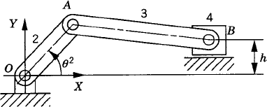
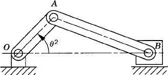
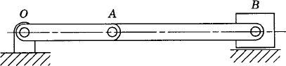
Figure 15 shows a four-bar linkage. Body 1 is the fixed link or the ground, body 2 is the crankshaft OA, body 3 is the coupler AB, and body 4 is the rocker BC. Obtain an expression for the angular orientation, velocities, and accelerations of the coupler and the rocker in terms of the angular orientation, angular velocity, and angular acceleration of the crankshaft. Assuming that the angular velocity of the crankshaft is constant and is equal to 50 rad/s, determine the values of the angular coordinates, velocities and accelerations of the coupler and the rocker for different values of the angles of the crankshaft. Assume that the lengths of the crankshaft, coupler and the rocker are 0.2, 0.4, and 0.5 m, respectively, and the distance OC is 0.4 m.
Solution. The position vector of point C can be expressed in terms of the Cartesian coordinates of the rocker as
where R4 is the global position vector of the reference point of the rocker, which we select in this example to be point B, A4 is the transformation matrix of the rocker,
where R3 is the global position vector of the reference point of the coupler, which is selected in this example to be point A, A3 is the transformation matrix of the coupler,
where l2 is the length of the crankshaft. The vector R4 can then be written as
Using this equation, the global position vector of point C can be written as
From Fig. 15 it is clear that

where l1 is the distance OC. The preceding two equations lead to the following two scalar equations:
These two equations are called the loop closure equations of the four-bar linkage. They can be used to express the angles θ3 and θ4 in terms of the angle θ2. It is left to the reader to try to solve the loop closure equations and determine θ3 and θ4 as a function of the crank angle θ2.
Following the procedure described in the preceding example, one can show that the global velocity vector of point B on the coupler is
The velocity of point C, which, in this example, is equal to zero can be expressed in terms of the velocity of point B as
Using Eqs. 27 and 31 and the fact that v4B = v3B and v4C = 0, one obtains

which can be rearranged and written as
or
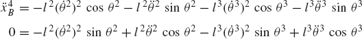
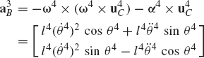
Following a procedure similar to the one described in the preceding example, one can show that the acceleration of point B is

The acceleration of point C on the rocker is
Since C is a fixed point, one has a4C = 0, and accordingly,
which leads to
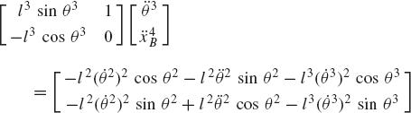
Substituting Eq. 69 into Eq. 68, one obtains the following scalar equations:
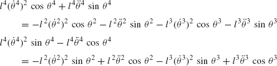
Assuming that θ3, θ4,
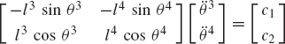
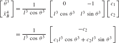
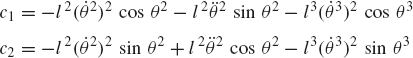
where c1 and c2 are
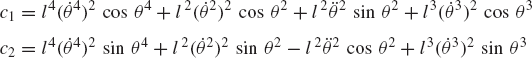
Equation 70 can be solved for the angular accelerations
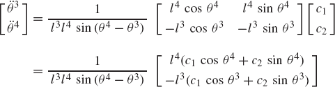
Using the dimensions of the mechanism and the kinematic equations presented in this example, the angular coordinates, velocities and accelerations of the links can be determined as functions of the crank angle as shown in Table 2. The angles presented in this table are in radians, the angular velocities are in rad/s, and the angular accelerations are in rad/s2.
The position kinematic equations obtained in the preceding example can be used to express the orientations of the coupler and the rocker in terms of the crank angle θ2. One of the important considerations in the design of many of the four-bar linkages is to ensure that the crankshaft can rotate a complete revolution. In order to determine whether the input crank of the four-bar mechanism can make a complete revolution, Grashof's law can be used. This law states that, for a planar four-bar linkage, if the sum of the lengths of the shortest and longest links is less than the sum of the lengths of the other two links, then a continuous relative motion between two links can be achieved. Let s and l be, respectively, the lengths of the shortest and longest links, and p and q be the lengths of the other two links. According to Grashof's law, the shortest link will rotate continuously if
Table 3.2. Four-Bar Mechanism
θ2 | θ3 | θ4 | ||||
|---|---|---|---|---|---|---|
0.157E + 01 | 0.795E + 00 | 0.495E + 01 | −0.702E + 01 | 0.165E + 02 | 0.106E + 04 | 0.717E + 03 |
0.177E + 01 | 0.774E + 00 | 0.503E + 01 | −0.314E + 01 | 0.188E + 02 | 0.901E + 03 | 0.441E + 03 |
0.197E + 01 | 0.769E + 00 | 0.510E + 01 | 0.255E + 00 | 0.201E + 02 | 0.803E + 03 | 0.228E + 03 |
0.217E + 01 | 0.776E + 00 | 0.518E + 01 | 0.334E + 01 | 0.206E + 02 | 0.745E + 03 | 0.593E + 02 |
0.237E + 01 | 0.795E + 00 | 0.527E + 01 | 0.625E + 01 | 0.206E + 02 | 0.712E + 03 | −0.768E + 02 |
0.257E + 01 | 0.826E + 00 | 0.535E + 01 | 0.905E + 01 | 0.201E + 02 | 0.693E + 03 | −0.187E + 03 |
0.277E + 01 | 0.868E + 00 | 0.543E + 01 | 0.118E + 02 | 0.191E + 02 | 0.677E + 03 | −0.274E + 03 |
0.297E + 01 | 0.920E + 00 | 0.550E + 01 | 0.145E + 02 | 0.179E + 02 | 0.657E + 03 | −0.339E + 03 |
0.317E + 01 | 0.983E + 00 | 0.557E + 01 | 0.170E + 02 | 0.164E + 02 | 0.624E + 03 | −0.383E + 03 |
0.337E + 01 | 0.106E + 01 | 0.563E + 01 | 0.194E + 02 | 0.149E + 02 | 0.577E + 03 | −0.408E + 03 |
0.357E + 01 | 0.114E + 01 | 0.569E + 01 | 0.216E + 02 | 0.132E + 02 | 0.515E + 03 | −0.418E + 03 |
0.377E + 01 | 0.123E + 01 | 0.574E + 01 | 0.235E + 02 | 0.115E + 02 | 0.438E + 03 | −0.417E + 03 |
0.397E + 01 | 0.133E + 01 | 0.578E + 01 | 0.251E + 02 | 0.986E + 01 | 0.347E + 03 | −0.413E + 03 |
0.417E + 01 | 0.143E + 01 | 0.582E + 01 | 0.263E + 02 | 0.822E + 01 | 0.243E + 03 | −0.411E + 03 |
0.437E + 01 | 0.154E + 01 | 0.585E + 01 | 0.270E + 02 | 0.656E + 01 | 0.123E + 03 | −0.418E + 03 |
0.457E + 01 | 0.165E + 01 | 0.587E + 01 | 0.273E + 02 | 0.484E + 01 | −0.193E + 02 | −0.445E + 03 |
0.477E + 01 | 0.175E + 01 | 0.589E + 01 | 0.268E + 02 | 0.296E + 01 | −0.200E + 03 | −0.503E + 03 |
0.497E + 01 | 0.186E + 01 | 0.589E + 01 | 0.256E + 02 | 0.751E + 00 | −0.444E + 03 | −0.612E + 03 |
0.517E + 01 | 0.196E + 01 | 0.589E + 01 | 0.231E + 02 | 0.204E + 01 | −0.799E + 03 | −0.803E + 03 |
0.537E + 01 | 0.204E + 01 | 0.588E + 01 | 0.189E + 02 | −0.586E + 01 | −0.135E + 04 | −0.113E + 04 |
0.557E + 01 | 0.211E + 01 | 0.584E + 01 | 0.121E + 02 | −0.113E + 02 | −0.222E + 04 | −0.167E + 04 |
0.577E + 01 | 0.214E + 01 | 0.579E + 01 | 0.734E + 02 | −0.195E + 02 | −0.356E + 04 | −0.250E + 04 |
0.597E + 01 | 0.210E + 01 | 0.568E + 01 | −0.169E + 02 | −0.314E + 02 | −0.512E + 04 | −0.333E + 04 |
0.617E + 01 | 0.199E + 01 | 0.553E + 01 | −0.389E + 02 | −0.447E + 02 | −0.544E + 04 | −0.295E + 04 |
0.637E + 01 | 0.179E + 01 | 0.533E + 01 | −0.562E + 02 | −0.516E + 02 | −0.273E + 04 | −0.184E + 03 |
0.657E + 01 | 0.156E + 01 | 0.513E + 01 | −0.593E + 02 | −0.457E + 02 | −0.100E + 04 | −0.290E + 04 |
0.677E + 01 | 0.134E + 01 | 0.498E + 01 | −0.510E + 02 | −0.314E + 02 | 0.278E + 04 | 0.393E + 04 |
0.697E + 01 | 0.116E + 01 | 0.488E + 01 | −0.393E + 02 | −0.163E + 02 | 0.286E + 04 | 0.346E + 04 |
0.717E + 01 | 0.102E + 01 | 0.484E + 01 | −0.288E + 02 | −0.417E + 01 | 0.236E + 04 | 0.261E + 04 |
0.737E + 01 | 0.922E + 00 | 0.484E + 01 | −0.205E + 02 | 0.471E + 01 | 0.184E + 04 | 0.186E + 04 |
0.757E + 01 | 0.853E + 00 | 0.488E + 01 | −0.140E + 02 | 0.109E + 02 | 0.143E + 04 | 0.128E + 04 |
0.777E + 01 | 0.808E + 00 | 0.493E + 01 | −0.887E + 01 | 0.152E + 02 | 0.115E + 04 | 0.858E + 03 |
This inequality has to be satisfied, otherwise none of the links will make a complete revolution relative to the other links. If link 2 in the four-bar linkage (Fig. 15) can make a complete revolution while link 4 oscillates, the mechanism is called a crank-rocker linkage. If both link 2 and link 4 oscillate between limits, the mechanism is called a double-rocker linkage.
Grashof's law makes no mention of which link is fixed or of the order in which the links are connected. Several kinematic inversions of the four-bar mechanism, however, can be obtained by selecting which link is to be fixed and by arranging the connectivity of the links based on their lengths. When the crank is the shortest link and it is adjacent to the fixed link, the resulting mechanism is of the crank-rocker type. If the shortest link is the fixed link, one obtains the double-crank mechanism, which is also called a drag-link mechanism. When the link opposite to the shortest link is the fixed link, one obtains again the double-rocker mechanism. The double-rocker mechanism is also obtained if the sum of the lengths of the shortest link and longest link is larger than the sum of the other two links.
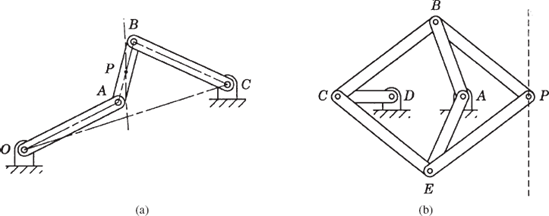
It is clear in the case of the four-bar linkage of Fig. 15 that any point on the crankshaft OA or the rocker BC moves on a circular arc that has a radius equal to the distance between this point and the fixed points O and C, respectively. During the dynamic motion of the mechanism, any point on the coupler of the four-bar linkage generates a path, called a coupler curve, that depends on the location of this point. Clearly, the two paths generated by points A and B are simple circles. Four-bar mechanisms can be designed such that a point on the coupler link moves in a straight line. Such mechanisms are called straight-line mechanisms. An example of an approximate straight-line mechanism is the four-bar Watt's mechanism shown in Fig. 16a. If, in this mechanism, the position of point P on the coupler is such that the ratio of the lengths of the segments AP and PB is inversely proportional to the ratio of the lengths of the links OA and BC, respectively, then the coupler curve of point P is an approximate straight line. A mechanism that generates an exact straight line is the Peaucellier mechanism shown in Fig. 16b. This mechanism consists of eight links including the fixed link. As pointed out in Chapter 1, if the lengths of link AB and link AE are equal, lengths of links BC, BP, EC, and EP are equal, and the length of link AD is equal to the distance CD, point P will trace out an exact straight-line path. Straight-line mechanisms are used in many mechanical system applications such as gear switch equipment and engine indicators.
The classical kinematic approaches, both graphical and analytical, can also be used in the analysis of mechanisms with Coriolis acceleration. The use of the classical analytical approach in the analysis of such mechanisms is demonstrated by the following examples.
Example 3.5
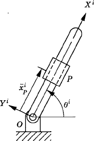
Figure 17 shows a block P that slides on a slender rod i. The rod is connected to the ground by a pin joint at O and rotates with angular velocity
Solution. We first select the rod coordinate system to be XiYi with origin at O. The position vector of the block with respect to this coordinate system is
Since the block is moving with respect to the rod, its velocity is described by Eq. 46 as
Since O is a fixed point, viO = 0, and
in which
and
The absolute velocity of the block P can then be written as
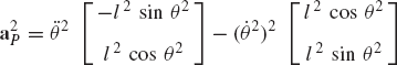
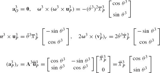
The absolute acceleration vector of the block P can be obtained by differentiating the absolute velocity vector viP or by using the general expression of Eq. 50. Both methods yield the same results. In this example, the general expression of Eq. 50 is used. Since point O is fixed, the absolute acceleration of point O is equal to zero, that is,
In this case, the acceleration of point P takes the form
in which
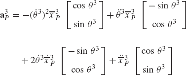
Substituting these equations into the expression for the acceleration of point P, one obtains
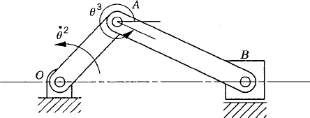
Example 3.6
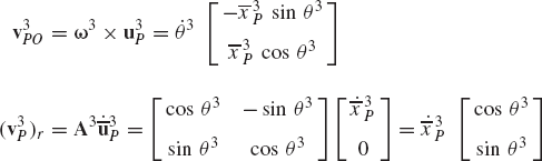
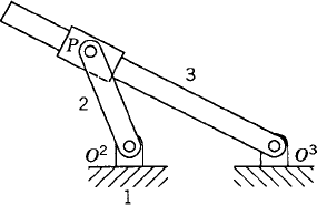
Figure 18 shows two rotating rods that are connected by the slider block P. Given the angular velocity and angular acceleration of rod 2, determine the angular velocity and angular acceleration of rod 3 and the relative velocity and acceleration of the slider block P with respect to rod 3.
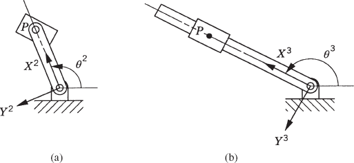
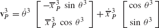
Solution. First we perform the velocity analysis of the mechanism. We first consider rod 2 as shown in Fig. 19a. The absolute velocity of point P on rod 2 is
where v2O = 0, and
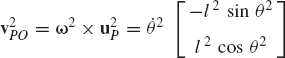
Here, l2 is the length of link 2. The absolute velocity of point P can then be written as
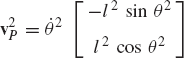
Due to the fact that the slider block P slides on link 3, the absolute velocity of point P can also be evaluated by analyzing the motion of link 3 shown in Fig. 19b. In this case, one has
Keeping in mind that point O3 is a fixed point, one has v3O = 0. One also has
where
Since v2P = v3P, one has
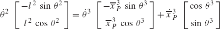
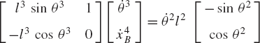
This equation can be written in a matrix form as
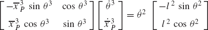
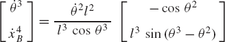
This matrix equation contains two scalar algebraic equations that can be solved for the two unknowns
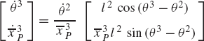
Having determined
where
The absolute acceleration of point P can then be written as
As the slider block P moves with respect to rod 3, the absolute acceleration of point P takes the form
where
The absolute acceleration of point P is
Using the fact that a2P = a3P, one obtains
The terms in this equation can be rearranged and written in a matrix form as
This matrix equation can be solved for the two unknowns
A careful examination of the classical solution procedures used for the position, velocity, and acceleration analysis of the mechanisms discussed in the examples presented thus far in this chapter reveals that, in general, there is an explicit or implicit use of a set of algebraic kinematic equations that describe the joint connectivity between the bodies of the system as well as specified motion trajectories. For instance, for the slider crank mechanism of Example 3, we explicitly or implicitly used the following algebraic equations and their derivatives
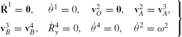
where R1 and θ1 are the coordinates of the ground (fixed link) R4y and θ4 are the vertical displacement and the angular orientation of the slider block, and ω2 is a known function of time. The last equation describes the constraint condition used to drive the crankshaft of the mechanism. Each one of the preceding equations was manipulated separately so as to yield a procedure which is tailored only for the analysis of the slider crank mechanism. Note that the number of algebraic equations given in Eq. 72 is 12 which is equal to the number of coordinates of the mechanism. The planar slider crank mechanism has four bodies (nb = 4); the ground (Body 1), the crankshaft (Body 2), the connecting rod (Body 3), and the slider block (Body 4). The total number of coordinates of the mechanism is n = 3 × nb = 12. That is, the total number of kinematic equations is equal to the total number of coordinates, and this number is equal to the number of constraint equations given in Eq. 72.
Another alternative, yet equivalent approach is to combine the preceding equations and solve them simultaneously using matrix and computer methods. While this alternative approach is not different in principle from the methods used in the preceding examples, its use, as demonstrated in the remainder of this chapter, allows us to develop a systematic computer procedure that can be used in the kinematic analysis of varieties of multibody system applications. The kinematic relationships that describe the joint connectivity between bodies as well as specified motion trajectories will be formulated so as to obtain a number of algebraic equations equal to the number of the system coordinates. The resulting system of loosely coupled equations can be solved efficiently using numerical techniques.
As pointed out previously, the planar motion of an unconstrained rigid body can be described using three independent coordinates. Two coordinates define the translation of the body as represented by the displacement of the origin of a selected body reference and one coordinate defines the orientation of the body. The translational motion of the rigid body i can be defined by the vector Ri that describes the position of the origin of the body reference with respect to the global coordinate system, while the orientation of the body can be described using the angle θi. Using the three coordinates
where
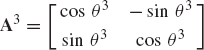
is the position vector of the arbitrary point defined in the body coordinate system, and Ai is the transformation matrix from the body coordinate system to the global coordinate system defined in terms of the angle of rotation θi as
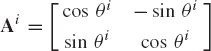
In this chapter and in the following chapters, the coordinates Ri and θi are referred to as the absolute Cartesian generalized coordinates of the rigid body i.
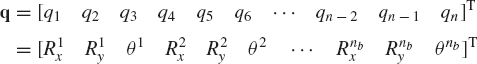
A multibody system consisting of nb unconstrained rigid bodies has 3 × nb independent generalized coordinates. The vector q of the generalized coordinates of the multibody system is then defined as
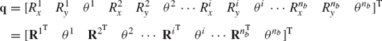
which can also be written in the following form:
where

is the vector of generalized coordinates of body i.
As previously mentioned, in the computational kinematic approach that will be used in this text, each body in the system is assigned three absolute Cartesian coordinates in the planar analysis and six absolute Cartesian coordinates in the spatial analysis. These coordinates define the translation and the orientation of the bodies in space. Therefore, in the planar analysis, the number of system coordinates is n = 3 × nb; whereas in the spatial analysis, the number of system coordinates is n = 6 × nb, where nb is the total number of bodies in the system. In order to solve for the system coordinates using the kinematic analysis, one must have a number of algebraic equations equal to the number of coordinates. These algebraic equations are the constraint equations imposed on the motion of the multibody system. By formulating the algebraic constraint equations in terms of the coordinates of the body, one can obtain a number of equations nc that is equal to the number of coordinates n. These position level equations can be solved for the coordinates using numerical methods as will be discussed in later sections of this chapter. By differentiating the constraint equations with respect to time, one obtains the constraint equations at the velocity level. This differentiation leads to a system of linear algebraic equations that can be solved for the velocities. A second differentiation defines the constraint equations at the acceleration level. These equations, which are linear in the accelerations, can be solved in a straightforward manner to determine the second derivatives of the system coordinates. It is, therefore, important to be able to formulate the algebraic equations of the constraints in terms of the system generalized coordinates.
Kinematic constraints that impose restrictions on the relative motion between bodies in the multibody systems are classified as joint constraints and driving constraints. Joint constraints, which are the result of restrictions imposed by the mechanical joints such as revolute, prismatic, cylindrical, and spherical joints, describe the connectivity between the multibody system components, and therefore, define the system topological structure. The formulation of the driving and joint constraint equations will be discussed in more detail in the following two sections.
While joint constraints are assumed to depend only on the system coordinates, driving constraints describe the specified motion trajectories, and therefore, may depend on the system generalized coordinates as well as time. An example of driving constraints is the specified motion of the crankshaft of a slider crank mechanism, as the one shown in Fig. 20. If the crankshaft is denoted as body 2, and it is assumed to rotate with a constant angular velocity, one has
where ω2 is a constant. The preceding equation is a differential equation that can be integrated to define a kinematic constraint equation that depends on the coordinate θ2 as well as time and can be written as
where t is time and θ2o is the initial angular position of the crankshaft. Equation 80 is an example of a simple constraint that can be imposed on the absolute coordinates of a body in the system. For body i in the system, one may encounter situations in which one or more of the following simple driving constraints must be imposed:
where f1(t), f2(t), and f3(t) are time-dependent functions and Rix, Riy, and θi are the absolute coordinates of the rigid body i.
More complex driving constraints arise in multibody system applications when the motion of an arbitrary point on a rigid body is prescribed. Specified trajectories in the analysis of robotic manipulators, numerically controlled machine tools, and railroad vehicles are examples of such driving constraints. For example, if the coordinates of a point Pi on the rigid body i are prescribed such that this point follows a given trajectory defined by the function
This equation, in the planar analysis, leads to two scalar equations that can be written in terms of the absolute coordinates of body i as
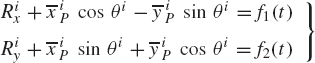
In these two equations which constrain the two global coordinates of point Pi, the first constraint specifies the horizontal motion of the point while the second specifies the vertical motion. If point Pi coincides with the origin of the body reference, that is,
Other types of driving constraints may result from imposing conditions on the relative motion between two bodies in the multibody system. For example, if the relative rotation between two bodies i and j in the system is specified, the constraint equation can be written as
where θi and θj are the angular orientation of bodies i and j, respectively, and f(t) is a known function of time. Similarly, if the relative displacement between points Pi and Pj on bodies i and j is specified, the resulting kinematic constraints can be classified as driving constraints and can be written as
where riP and rjP are, respectively, the global position vectors of points Pi and Pj, and
This vector equation has two scalar equations that describe the constraints between the coordinates of point Pi and point Pj.
In many multibody system applications, both joint and driving constraints exist. A simple example is the slider crank mechanism shown in Fig. 20. The mechanism has four joints; three revolute and one prismatic. A driving constraint similar to the one given by Eq. 80 can still be imposed on the motion of the crankshaft. It is important, however, to point out that the maximum number of driving constraints that can be imposed on the motion of a given system must not exceed the number of the system degrees of freedom. Driving constraints depend on the applications, and they may depend explicitly on time as demonstrated in this section. For this reason, general purpose multibody system computer programs provide user subroutines that allow the user to introduce these nonstandard constraints. In the kinematic analysis, the motion of the system is produced by the driving constraints. Associated with these driving constraints, there are driving constraint forces that represent actuator forces or motor torques. These driving constraint forces and torques can be systematically determined as will be explained when the subject of constrained dynamics is covered in later chapters of this book.
In this section, the formulation of joint constraint equations in terms of the absolute coordinates that describe the location and orientation of the rigid bodies with respect to a fixed global coordinate system is discussed. Only planar motion constraints are considered in this section. The formulation of the joint constraints in the spatial analysis is presented in Chapter 7.
A body that has zero degrees of freedom is called a ground or fixed link. The ground constraints imply that the body has no translational or rotational degrees of freedom. If body i is assumed to be a ground or a fixed link, the algebraic kinematic constraints are given by
where c1, c2, and c3 are constants. The conditions of Eq. 87 eliminate the translational and rotational degrees of freedom of the body. These conditions can be combined into one vector equation as
where
When two bodies are connected by a revolute joint, only relative rotation between the two bodies is allowed. Figure 21 depicts two rigid bodies i and j that are connected by a revolute joint at point P which is called the joint definition point. It is clear from the figure that the position vector of this point as defined using the absolute coordinates of body i must be equal to the position vector of the same point as defined in terms of the absolute coordinates of body j. The kinematic constraint conditions of the revolute joint can then be stated mathematically as
or equivalently,
where
which yields the two scalar equations
These are the two constraint equations that eliminate the freedom of the relative translation between the two bodies.
If a rigid body i is connected to the ground by a revolute joint, Eq. 90 reduces in this special case to
where c is a constant vector that defines the absolute Cartesian coordinates of point P. The kinematic conditions of Eq. 93, which are sometimes called point constraints, imply that point P on the rigid body i is a fixed point.
The prismatic joint, which is also called the translational joint, allows only relative translation between the two bodies along the joint axis. The constraint equations for the prismatic joint reduce the number of degrees of freedom of the system by two. Figure 22 depicts two bodies i and j that are connected by a prismatic joint. A constraint equation that eliminates the relative rotation between the two bodies can be written as
where c is a constant defined by the equation c = θio − θjo in which θio and θjo are the initial orientation angles of bodies i and j, respectively.
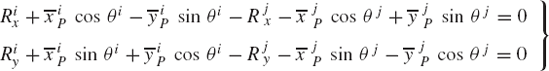
A second condition for the prismatic joint is required in order to eliminate the relative translation between the two bodies along an axis perpendicular to the joint axis. To formulate this condition, the two perpendicular vectors rijP and hi are defined. The vector rijP connects two arbitrary points Pi and Pj that lie on the axis of the prismatic joint as shown in the figure. Point Pi is defined on body i, and therefore, its coordinates are fixed with respect to the coordinate system of body i, while point Pj is defined on body j, and accordingly, its coordinates are fixed in the coordinate system of body j. The vector hi, which is assumed to be perpendicular to the joint axis, may be defined on body i and can be selected to be the vector joining points Pi and Qi, as shown in the figure. The vectors rijP and hi can then be defined in terms of the coordinates of body i and body j as
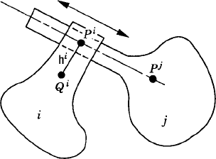
where
This is a scalar equation that can be written in a more explicit form using Eq. 95.
One can combine the two constraint equations of the prismatic joint given by Eqs. 94 and 96 in one vector equation as
While the first equation in Eq. 97 is a linear function of the rotational coordinates of body i and body j, the second equation is a nonlinear equation in the absolute coordinates of the two bodies.
Example 3.7
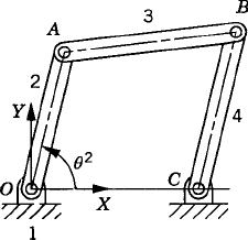
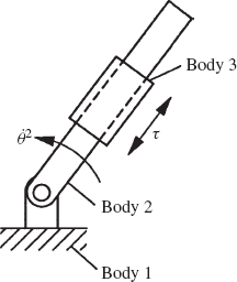
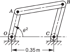
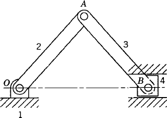
Derive the algebraic kinematic constraint equations of the three-body system shown in Fig. 23, and determine the number of the system degrees of freedom.
Solution. The absolute coordinates of body i in the system are assumed to be Rix, Riy, and θi, i = 1, 2, 3. The ground constraints are
where c1, c2, and c3 are constants. If the axes of the coordinate system of body 1 are assumed to coincide with the axes of the global coordinate system, the constants c1, c2, and c3 are identically zeros. The two kinematic constraint equations for the pin (revolute) joint at O can be written in a vector form as
where
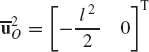
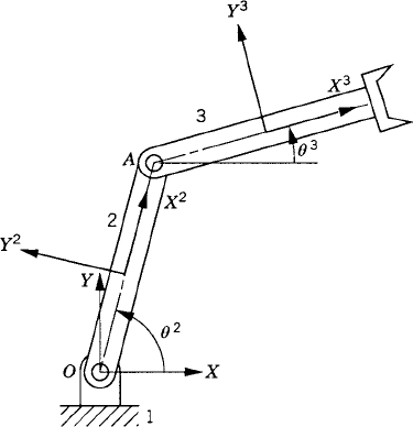
where l2 is the length of the rod 2. The constraint equations for the revolute joint at O lead to
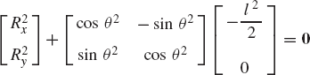
or
Similarly, the constraint equations for the revolute joint at A are given by
Assuming that body 3 is a uniform rod of length l3 with the origin of its body coordinate system attached to its center, one has
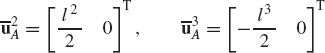
which can be used to define the kinematic constraints of the revolute joint at A as
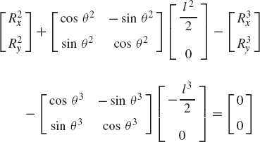
or
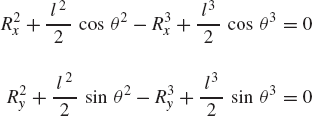
The kinematic constraint equations of the system can be written in a vector form as
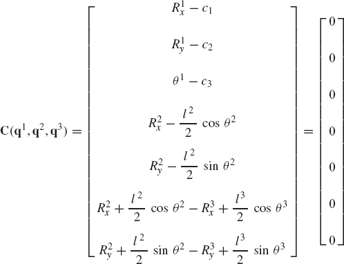
where
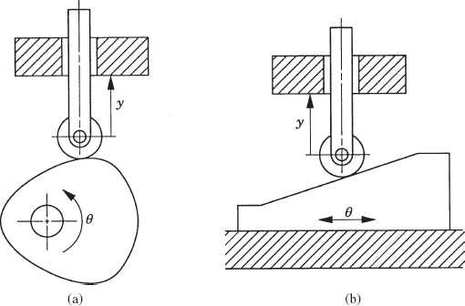
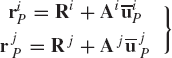
A cam is a mechanical component that is used to drive another component called a follower. The cams are convenient and versatile mechanical devices for motion generation because of their various geometrical shapes and the various existing combinations between the cam and its follower. The cam and the follower mechanism constitute an important part in many mechanism systems such as instruments, internal combustion engines, and machine tools. Cams may be classified according to their basic shapes or according to the basic shapes of the followers. Figure 24 shows two different types of cam systems classified according to the shape of the cam, while Fig. 25 shows different types of cam systems classified according to the shape of the follower element. As the result of the rotation of the camshaft, the output motion of the follower can be translating or rotating motion. In most cam applications, as shown in Figs. 24 and 25, the shape of the follower in the contact region with the cam is chosen to be of simple geometry, while the desired motion is achieved by the proper design of the cam shape. The cam and follower, however, must remain in contact at all times. This can be achieved by using a suitable spring, by utilizing the effect of gravity, or by using any mechanical constraints.
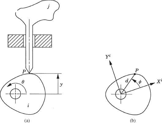
In order to demonstrate the formulation of the algebraic kinematic constraints in the case of cam systems, as an example, the offset reciprocating knife-edge follower shown in Fig. 26 is first considered. The cam and the follower denoted, respectively, as bodies i and j may be connected with other bodies in a system by different types of joints. The point of contact between the cam and the follower is assumed to be point P, where point P is a fixed point in the follower coordinate system. The coordinates of this point, however, in the cam coordinate system depend on the cam shape. The global position of point P as defined using the absolute coordinates of the cam (body i) and the follower (body j) can be written as
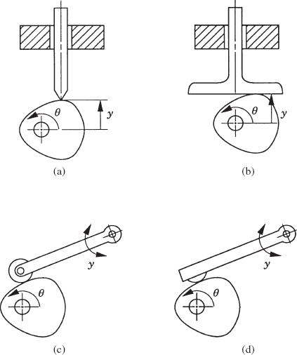
where
This equation defines the exact nature of the shape of the cam. By using the functional relationship of Eq. 99, the vector
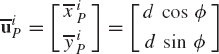
which implies that any point on the surface of the cam corresponds to a unique set of the two parameters d and ϕ, which define the shape of the cam that produces the desired follower motion. The shape of the cam can be defined by expressing d analytically or numerically in terms of the angle ϕ as
Consequently, the coordinates of any point on the cam surface can be defined in terms of the angle ϕ. In the computer implementation, Eq. 101 can be described numerically using the cubic spline functions.
By using Eq. 98, the kinematic constraint equations for the cam system shown in Fig. 26 can be written as
Note that in addition to the system generalized coordinates, the geometric nongeneralized surface parameter ϕ that defines the cam surface was introduced in order to be able to formulate the constraints of Eq. 102 (Shabana and Sany, 2001). Therefore, the number of unknown variables increases as a result of including the geometric parameter ϕ, and the two constraint equations of Eq. 102 eliminate only one degree of freedom from the original n coordinates of the system. That is, one of the equations in Eq. 102 can be used to eliminate the parameter ϕ from the other equation, leading to only one constraint equation that is a function of the original generalized coordinates of the system. By so doing, it becomes clear that the system of Eq. 102 is equivalent to one equation that is function of the generalized coordinates of the cam and the follower, and therefore, the resulting cam/follower constraint equations eliminate only one degree of freedom of the system.
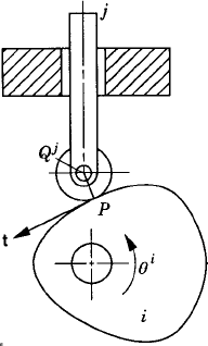
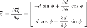
Another type of cam systems is the roller follower cam, shown in Fig. 27. The contact point between the cam and the roller is point P, while the center of the roller is defined by point Qj on the follower, which is denoted as body j. The vector n connecting the two points P and Qj is perpendicular to the vector t, which is tangent to the roller at the contact point. The two kinematic constraint equations for this type of cam system can be written as
where r is the radius of the roller and the vector n is defined in terms of the absolute coordinates of the cam and the follower as
The vectors
The tangent vector t in Eq. 103 can also be defined in the cam coordinate system using Eq. 100 as
Using this equation, the tangent vector can be defined in the global coordinate system as
Example 3.8
Derive the kinematic constraint equations of the offset flat-faced follower shown in Fig. 28.
Solution. Let point Pi and Pj denote the contact point on the cam and the flat-faced follower, respectively. Two perpendicular vectors n and t are defined at the contact point. The vector
This vector must remain perpendicular to n, that is, the first constraint equation is given by
Another vector t that is tangent to the cam at point Pi may be defined. This vector is also perpendicular to the vector n, leading to the second condition
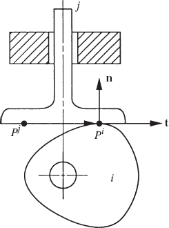
Using the preceding two equations, the constraint equations for this type of cam can be written in a vector form as
While the second condition guarantees that the flat-faced follower remains parallel to the tangent to the cam surface at the contact point, the first condition guarantees that there is no separation or penetration between the cam and the follower. The vector rijP depends on the absolute coordinates of the cam and the follower as well as the shape of the cam, while the vector t depends on the absolute coordinates and the shape of the cam only.
Gears are widely used in machines for the purpose of transmission of rotary or rectilinear motion from one component to another (Litvin, 1994). Gears are used in a variety of industrial and technological applications such as automobiles, tractors, electric drills, helicopter rotor systems, machine tools, kitchen appliances, aircrafts, alarming clocks, and others. The theory of gearing is based on the fact that power can be transmitted from one body to another if the bodies have rolling contact. A rotary motion, for instance, can be transmitted from one body to another by friction if the two bodies are pressed against each other. If the friction force is high enough such that the two bodies roll without slipping, the velocities of the two bodies at the point of contact are equal. In this case, there is a definite relationship between the input and the output motions. The friction between the two bodies can be increased by increasing the roughness of the two surfaces in contact. A more reliable approach is to cut teeth on the surfaces of the two bodies. In this case, motion is transmitted by successive engagement of the teeth. Spur gears as shown in Fig. 29a are formed if the teeth are cut in a direction parallel to the axis of rotation. Gears can also be formed by cutting the teeth along a helix generated around the axis of the gear. In this case, the gear is called a helical gear and is shown in Fig. 29b. Both spur and helical gears are used to transmit power between two parallel axes. If the diameter of one of the spur gears goes to infinity, one obtains the rack and pinion system. Another type of gear that is widely used are bevel gears which, as shown in Fig. 29c, are cut from cones and are used in the case of intersecting shafts. In the case of nonintersecting and nonparallel shafts, the skew gears, hypoid gears, and worm gears (Fig. 29d) are used for the purpose of power transmission.
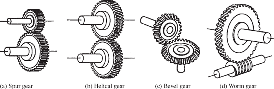
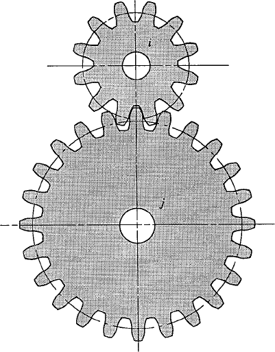
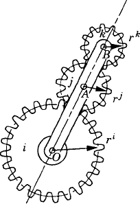
The simple case of spur gears is considered as an example in this section to demonstrate the formulation of the kinematic constraints in gear systems. Figure 30 shows a pair of spur gears which are assumed to be attached to a third body k. The condition that no sliding occurs between the two gears i and j at the contact point can be written as
where ai and aj are, respectively, the radius of the pitch circles of gears i and j. Integrating Eq. 106, one obtains the kinematic constraint equation for the spur gear system as
in which θio, θjo, and θko are the initial angular orientations of bodies i, j, and k, respectively.
If body k does not rotate, that is, θk=θko, Eq. 107 reduces to
The formulation of the kinematic constraints for other types of gears can be developed using a similar procedure as demonstrated by the following example.
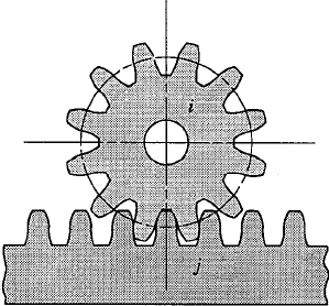
Example 3.9
Figure 31 shows a rack-and-pinion mechanism in which the pinion is denoted as body i while the rack is denoted as body j. The pinion is assumed to have only rotational motion about its own axis, while the rack is assumed to have only translational motion along the horizontal direction. The condition at the point of contact that ensures no sliding between the two bodies is given by
where ai is the radius of the pitch circle of the pinion,
where θio and
The formulations of the algebraic constraint equations presented in the preceding sections are used in this section to develop computer methods for the position, velocity, and acceleration analyses of multibody systems consisting of interconnected rigid bodies. In the analysis presented in this section, the configuration of the system is described by n coordinates, which can be written in a vector form as
In the planar analysis, if the system consists of nb bodies, and the absolute coordinates are selected to describe the system configuration, one has n = 3 × nb and the coordinates are defined as
In multibody system applications, these coordinates are not independent as the result of the kinematic constraint equations that describe system joints as well as specified motion trajectories. Examples of these constraints are the driving constraints, prismatic joints, revolute joints, and cam and gear constraints discussed in the preceding sections. These constraint equations can be written in a vector form as
where nc is the total number of constraint equations and t is time.
There are two cases that are encountered in the dynamic analysis of multibody systems. In the first case, the number of linearly independent constraint equations is equal to the number of the system coordinates, that is, nc = n. This situation arises when all the degrees of freedom of the system are prescribed using driving constraints. For example, a slider crank mechanism that consists of four bodies (including the ground) has 12 absolute coordinates. The three ground constraints, the three revolute joints, and the prismatic joint in the mechanism make the number of the degrees of freedom of the mechanism equal to one. One may select this degree of freedom to be the crank angle. If a driving constraint is used to specify the angular velocity of the crankshaft, the number of joint constraints plus the driving constraint becomes equal to 12, equal to the number of absolute coordinates of the system. When the number of constraint equations is equal to the number of system coordinates, the system is said to be kinematically driven.
In the second case, the number of constraint equations including the driving constraints is less than the number of the system coordinates, that is, nc < n. This situation arises when some of the degrees of freedom of the system are dynamically driven using force inputs. In this case, some of the degrees of freedom are not specified, and the system in this case is said to be dynamically driven. In the case of a dynamically driven system, a force analysis is required in order to obtain the position, velocity, and acceleration of the system components.
In this chapter, only kinematically driven systems are discussed. Dynamically driven systems are discussed in later chapters when the force analysis of multibody systems is considered. In the case of kinematically driven systems, the vector of the constraint equations, defined by Eq. 111, includes the joint and driving constraints as demonstrated by the following simple example.
Example 3.10
For the three-body system of Example 7, bodies 2 and 3 are assumed to rotate with constant angular velocities
Solution. If the absolute coordinates are used, the number of coordinates n is equal to 9 and the number of the joint constraints is equal to 7. By imposing constraints on the angular velocities of bodies 2 and 3, the system becomes kinematically driven. The two driving constraints
can be integrated, yielding
where θ2o and θ3o are the initial angular orientations of bodies 2 and 3, respectively. These two driving constraint equations can be combined with the joint constraints obtained in Example 7, leading to
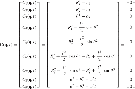
Given ω2, ω3, θ20, and θ30, the vector of constraints of the preceding equation defines nine algebraic equations that can be solved for the nine coordinates of the system Rix, Riy, and θi, i = 1, 2, 3.
For kinematically driven systems, the total number of constraint equations nc is equal to the number of system coordinates n. Consequently, the vector of the constraint equations defined by Eq. 111 contains n algebraic equations that describe joint constraints as well as driving constraints. This vector of the constraint equations represents n scalar equations that can be solved for the n unknown coordinates of Eq. 109. The equations, however, can be nonlinear functions of the system coordinates and time, a fact which was demonstrated in the preceding example where nonlinear trigonometric functions of the system coordinates appear in the algebraic kinematic constraint equations. Because a closed form solution cannot be obtained, in general, in the case of nonlinear systems; numerical methods are often used.
The numerical procedure often used for solving a system of nonlinear algebraic equations is the Newton-Raphson algorithm. This iterative procedure which can be employed to solve the nonlinear kinematic constraint equations starts by making an estimate of the desired solution vector. If this estimate at certain point in time t is denoted as qi, the exact solution can be written as qi + Δ qi. By using Taylor's theorem, the vector of constraint equations defined by Eq. 111 can be written as
where
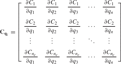
For a kinematically driven system, the Jacobian matrix is a square matrix since nc = n, and additionally, if the constraint equations are assumed to be linearly independent, Cq is a nonsingular matrix. If the vector qi + Δqi is assumed to be the desired exact solution, C(qi + Δqi, t)=0, and Eq. 112 reduces to
If the assumed solution is close to the exact solution, the norm of the vector Δqi becomes small and higher-order terms in the vector Δq in Eq. 114 can be neglected. This assumption defines the first-order approximation of Eq. 114 as
which yields
Since the constraint Jacobian matrix Cqi is assumed to be nonsingular, Eq. 116 can be solved for the vector of Newton differences Δqi. This vector can be used to iteratively update the vector of the system coordinates as
where i is the iteration number. The updated vector qi+1 can then be used to reconstruct Eq. 116 and solve this system of equations for the new vector of Newton differences Δqi+1, which can be used again to update the vector of the system coordinates, thus defining the vector qi+2. This process continues until the norm of the vector of Newton differences or the norm of the vector of constraint equations becomes less than a specified tolerance, that is,
where ɛ1 and ɛ2 are specified tolerances and k is the iteration number.
It is important to mention at this point that due to the fact that the Newton-Raphson method does not always converge, one must specify an upper limit on the number of iteractions used in this numerical algorithm. Failure to achieve convergence may be due to several factors, such as the initial estimate of the desired solution is not close enough to the exact solution, an error is made in the definition of the system constraints, and/or the multibody system is close to a singular configuration.
Example 3.11
For the three-body system of Example 10, it was shown that the vector of constraint equations is

where the vector q is selected to be the vector of absolute coordinates given by
The Jacobian matrix as defined by Eq. 113 can be developed for this system as
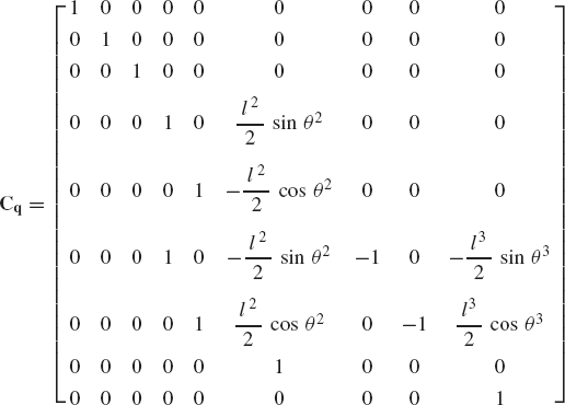
The matrix Cq is a square matrix, since the number of the constraint equations nc is equal to the number of coordinates n.
Differentiating the vector of constraint equations defined by Eq. 111 with respect to time, and using the chain rule of differentiation leads to
where Cq is the constraint Jacobian matrix defined by Eq. 113 and Ct is the vector of partial derivative of the constraint equations with respect to time. This vector is defined as
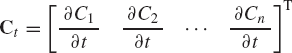
If the constraint equations are not explicit functions of time, the vector Ct is identically the zero vector.
Since the coordinates of the system components are assumed to be known from the position analysis, the Jacobian matrix Cq and the vector Ct which can be functions of the coordinates and time only can be evaluated. Equation 119, which can be considered as a linear system of algebraic equations in the velocity vector
Because Cq is assumed to be a square and nonsingular matrix in the case of kinematically driven systems, Eq. 121 can be solved for the velocity vector
The acceleration equations can be obtained by differentiating Eq. 119 with respect to time, leading to
This equation, by using the chain rule of differentiation, yields
This is a linear system of algebraic equations in the acceleration vector
where the vector Qd absorbs terms that are quadratic in the velocities and is defined as
Having determined the coordinate and velocity vectors q and
Example 3.12
For the three-body system of Example 11, one can verify that the vector Ct of Eq. 120 is given by
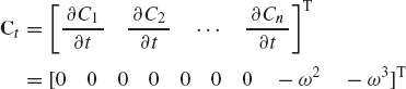
Using Eq. 121 and the constraint Jacobian matrix obtained in Example 11, it can be shown that the velocity vector
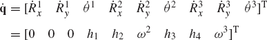
where
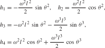
For the acceleration analysis, one has to evaluate the vector Qd of Eq. 125. For this system, if the angular velocities are assumed to be constant, the vector Ct is not an explicit function of the system coordinates or time. It follows that
The vector
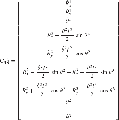
which can be used to define the matrix
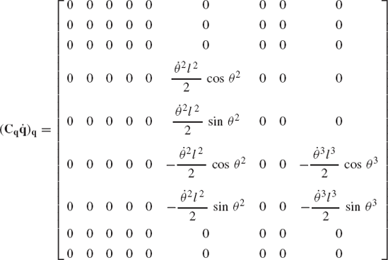
The vector
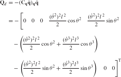
in which θ2, θ3,
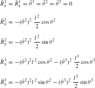
The results obtained in this simple example, using the general procedure outlined in this section, can also be obtained by simply differentiating the following kinematic relationships:
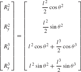
The formulation presented in the preceding section for kinematically driven systems leads to a number of nonlinear algebraic constraint equations which is equal to the number of coordinates. These constraint equations can be solved for the coordinates using a Newton-Raphson algorithm. Differentiation of the kinematic constraints once and twice leads to a linear system of algebraic equations in the velocities and accelerations which can be solved in a straightforward manner to determine the vector of system velocities and accelerations. Clearly, the number of resulting algebraic constraint equations depends on the choice of coordinates. Different sets of coordinates lead to different sets of algebraic equations. The number of the system degrees of freedom, however, remains the same, regardless of the type of coordinates used. As a consequence, the use of a larger number of coordinates requires the use of a larger number of constraint equations. Consider, for example, the four-bar mechanism shown in Fig. 32. One may select the system coordinates as
which is a subset of the absolute Cartesian coordinates of the mechanism. In this case, fewer constraint equations are required in order to describe the kinematic relationships between the angles θ2, θ3, and θ4. The constraint equations can be expressed in terms of these coordinates as
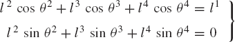
where l1 is the length OC. If the system is kinematically driven, a driving constraint must be introduced in order to control the degree of freedom of the system, thereby making the number of constraint equations equal to the number of coordinates. In this case, the general procedure outlined in the preceding section can still be used to solve a smaller system of equations as demonstrated by the following example.
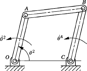
Example 3.13
For the four-bar linkage shown in Fig. 32, let l1 = OC = 0.35 m, l2 = 0.2 m, l3 = 0.35 m, and l4 = 0.25 m. The crankshaft of the mechanism is assumed to rotate with a constant angular velocity
Solution. Since the mechanism has only one degree of freedom, the coordinates θ2, θ3, and θ4 are not independent. They are related by the following loop-closure equations and the driving constraint equation
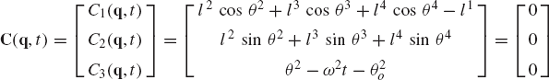
where
The Jacobian matrix of the constraint equations is
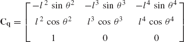
At t = 0.02 s, θ2 = 63° = 1.0996 rad. To start the numerical solution, we make an initial guess for the angles θ2, θ3, and θ4 as
Using the initial guess, the Jacobian matrix is
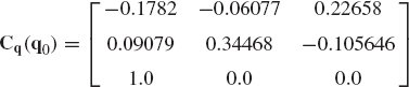
and the constraint equations are
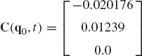
For this mechanism, Eq. 116 can be written as
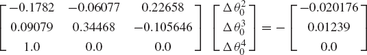
It is clear that Δθ20 = 0, and
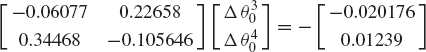
which can be solved for Δθ30, and Δθ40 as
The vector of the system coordinates can be updated according to Eq. 117 as
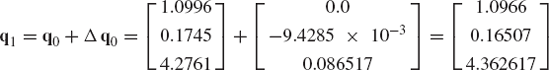
Using the vector
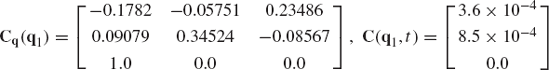
Equation 116 yields
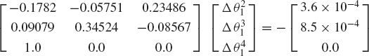
The solution of this system of equations yields
We may define the norms of C and Δq as
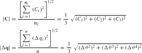
where nc and n are, respectively, the number of constraint equations and the number of coordinates. It follows that
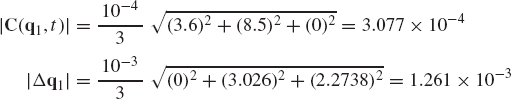
Since the norms of C and Δq1 are relatively small, one may decide to accept q1 as the correct answer for the position analysis and proceed to perform the velocity analysis. In this example, the vector Ct is
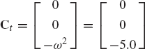
Using the Jacobian matrix previously evaluated at q = q1, the linear algebraic velocity equations can be written as
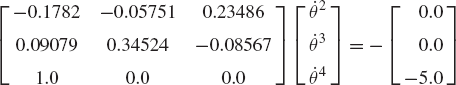
This equation defines the angular velocities
One can verify that the vector Qd of Eq. 124 is given for this example by
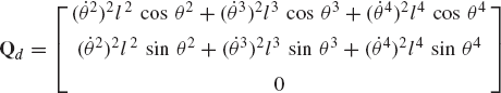
Using the values of the coordinates and velocities obtained previously in the position and velocity analyses at time t = 0.02s, the vector Qd can be evaluated as
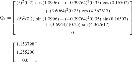
The linear algebraic equations for the angular accelerations can then be written as
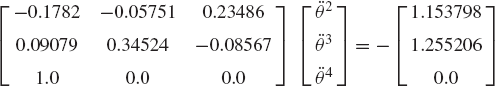
The solution of this system yields
The choice of the coordinates θ2, θ3, and θ4 in the preceding example was made by examining the topological structure of the four-bar mechanism. If another mechanism is considered, this set of coordinates is no longer suitable, and different constraint equations that take different forms must be formulated. For this reason, the choice of the coordinates based on the topological structure of the system under consideration makes it difficult to develop a general-purpose computer program for the kinematic analysis of multibody systems.
As discussed before, an alternative method for choosing the coordinates of the four-bar mechanism shown in Fig. 33 is to assume that the mechanism consists of four bodies, the fixed link or ground (body 1), the crankshaft (body 2), the coupler (body 3), and the rocker (body 4). Every body is assigned an identical set of coordinates that we select to be the absolute Cartesian coordinates Rix, Riy, and θi (i = 1, 2, 3, 4). As the result of this choice, the configuration of the mechanism is described using 12 coordinates, and consequently, the number of constraint equations increases. In this case, we have 11 joint constraints which include three ground constraints and eight constraints resulting from the revolute joints at O, A, B, and C. The formulation for the ground constraints can be simply written as
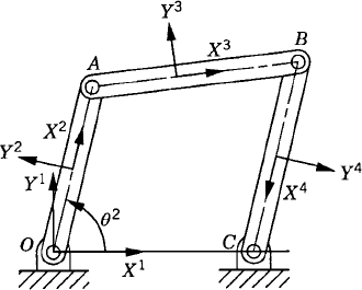
while the revolute joint constraints can be written as
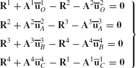
where
The use of the three absolute coordinates Rix, Riy, and θi for each body in the system, however, makes it possible to develop a general-purpose computer program for the dynamic analysis of multibody systems. In order to formulate the constraints of Eqs. 128 and 129, one only needs to identify which body is the ground, the bodies connected by the revolute joints, and the local position vectors of the joint definition points at O, A, B, and C. The local position vectors
If three absolute coordinates are used for each body in the mechanical system, the kinematic algebraic constraint equations of the joints can be formulated in a general form. This general formulation for the joint constraints does not depend on a specific application problem and can be used in the computer-aided kinematic analysis of varieties of multibody systems that consist of interconnected rigid bodies. Standard formulations for typical joints such as the ground constraints as well as revolute and prismatic joints can be implemented on the digital computer and made available for the analysis of a large class of multibody systems. For example, the kinematic constraints of a revolute joint between any pair of two rigid bodies i and j are given by
where P is the joint definition point. If one provides the body numbers, and the two constant vectors
The position, velocity, and acceleration analyses require the evaluation of the constraint Jacobian matrix. The Jacobian matrix of constraints such as the ground as well as revolute and prismatic joints can be also made as part of a standard constraint library in a general-purpose computer program. For instance, the Jacobian matrix of the revolute joint constraints of Eq. 130 can be written using vector notation as
where I is the 2 × 2 identity matrix, and Aiθ and Ajθ are the partial derivatives of Ai and Aj with respect to the rotational coordinates of bodies i and j, respectively. It is clear that the form of the Jacobian matrix of Eq. 131 remains the same for any pair of two rigid bodies connected by a revolute joint and this equation can be used for an arbitrary revolute joint in a multibody system. One only has to change the superscripts, which indicate the body numbers, and the constant vectors that define the local positions of the joint definition points.
For the velocity analysis, one has to evaluate the vector Ct of Eq. 121. This vector is equal to zero in the case of the revolute joint constraints of Eq. 130 because these constraints are not explicit functions of time. For the acceleration analysis, one must evaluate the vector Qd of Eq. 124. In the case of revolute joint, this vector reduces to
By using the Jacobian matrix of Eq. 131, one can show that
This equation has the same form for any pair of rigid bodies connected by a revolute joint.
Example 3.14
The constraint equations of the prismatic joint were defined by Eq. 97 as
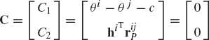
where
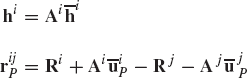
in which
The nonzero elements of the Jacobian matrix are
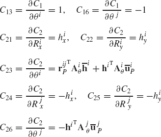
where hix and hiy are the components of the vector hi, that is,
The Jacobian matrix of the prismatic joint can then be defined as
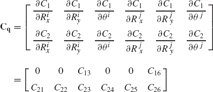
Since the prismatic joint constraints are not explicit functions of time, one has Ct = 0. It follows that
and
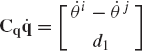
where
Hence,
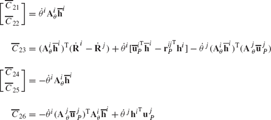
in which
The vector Qd can then be defined as

where Qd2 can be written explicitly as
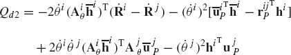
It is clear from the discussion presented in this section that the kinematic constraint equations of joints, such as revolute, prismatic, and other joints that are commonly used in multibody systems, can be derived systematically in a general form in terms of the absolute Cartesian coordinates. These joints can be made available as standard elements in a general-purpose computer program that can be used for the kinematic analysis of varieties of multibody system applications. The driving constraints, on the other hand, depend on the application and can be introduced to the general-purpose computer program by using user subroutines.
In what follows, a numerical algorithm that can be implemented in a general-purpose computer program for the position, velocity, and acceleration analyses of multibody systems is presented. The basic kinematic equations used in this numerical algorithm are first summarized.
In the position analysis, one needs to solve the system of nonlinear algebraic constraint equations
As pointed out in this chapter, a Newton-Raphson algorithm can be used for solving this equation. Thus, one must construct the matrix equation
where Δq is the vector of Newton differences.
The basic equations used in the velocity and acceleration analyses are
where the vector Qd is defined by Eq. 125.
The computational scheme for the analysis of kinematically driven systems that consist of interconnected rigid bodies is shown in Fig. 34 and proceeds in the following routine.
Step 1 At a given point in time t, an estimate for the desired solution is made. This estimate must be close to the exact solution in order to avoid divergence.
Step 2 The Jacobian matrix Cq and the vector of constraint equations C of Eq. 135 can be evaluated.
Step 3 Equation 135 is solved for the vector of Newton differences Δq.
Step 4 If the norm of the vector Δq or the norm of the vector of constraint equations C is small and less than specified tolerances (Eq. 118), proceed to step 5. Otherwise, update the vector of coordinates, that is, q = q + Δq and go to step 2 if the number of specified iterations is not exceeded.
Step 5 Having determined the vector of system coordinates, this vector can be used to evaluate the Jacobian matrix Cq and the vector Ct of Eq. 136.
Step 6 Equation 136 is a linear system of algebraic equations in the velocity vector. This system of equations can be solved for the vector

Step 7 Using the vectors q and
Step 8 Equation 137 is a linear system of algebraic equations in the acceleration vector. This equation can be solved for the vector

Step 9 Steps 1 through 8 are repeated until the simulation time ends.
For the most part, in a well-posed problem, there are no numerical problems encountered in the solution for the velocities and accelerations because only the solution of a linear system of equations is required. If the constraints are linearly independent, the constraint Jacobian matrix is a nonsingular square matrix, and consequently, there is a unique solution for Eqs. 136 and 137. Some numerical problems, however, may be encountered in the position analysis since an iterative scheme is required for the solution of a nonlinear system of equations. As pointed out previously, the Newton-Raphson algorithm may diverge if the assumed initial guess at each time step is not close enough to the exact solution. The use of the solution obtained in a previous step as the initial guess for the iterative Newton-Raphson algorithm at the current step may require the use of a very small step size in order to achieve convergence. One method for obtaining an improved initial approximation for the solution at a given step is to use the velocity and acceleration vectors obtained in the previous step to predict the solution. For example, the following truncated Taylor series expressed in terms of the coordinates, velocities, and accelerations at the previous step can be used:
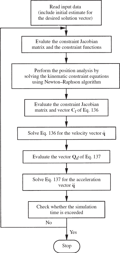
where qi,
In this section, the single-degree-of-freedom slider crank mechanism shown in Fig. 35 is used to demonstrate the use of the computer methods presented in the preceding section in the kinematic analysis of mechanism systems. The mechanism consists of four bodies; the fixed link denoted as body 1, the crankshaft OA denoted as body 2, the connecting rod AB denoted as body 3, and the slider block B denoted as body 4. Bodies 1 and 2 are connected by a revolute joint at O, bodies 2 and 3 are connected by a revolute joint at A, and bodies 3 and 4 are connected by a revolute joint at B. Bodies 1 and 4 are connected by a prismatic joint. The length of the crankshaft is assumed to be 0.15 m and the length of the connecting rod is assumed to be 0.35 m. As shown in Fig. 36 a body fixed coordinate system is attached to every body in the system including the ground. The vector of absolute coordinates of the slider crank mechanism is given by
Initially, the crankshaft is assumed to make an angle θ20 = 30°. The local position vectors of the revolute joint definition points are as follows:
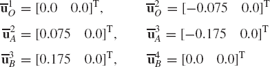
In this example, the prismatic constraints between bodies 1 and 4 reduce to
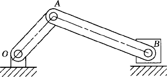
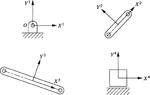
It is clear that the total number of joint constraints is 11 (three ground constraints, six revolute joint constraints, and two prismatic joint constraints). Recall that in the kinematic analysis, the number of coordinates must be equal to the number of constraint equations so as to have a kinematically driven system. There are two alternatives for introducing a driving constraint for this mechanism. The first alternative is to drive the mechanism by rotating the crankshaft, while in the second alternative, the mechanism is driven by moving the slider block. In each case, one driving constraint can be defined. This driving constraint, when it is added to the joint constraints, makes the total number of kinematic constraint equations equal to the total number of absolute coordinates of the mechanism. The simulation results presented in this section are obtained using the general purpose multibody computer program SAMS/2000 (Systematic Analysis of Multibody Systems) which is described in Chapter 9 of this book.
First, we consider the case where the angular velocity of the crankshaft is prescribed as
where f(t) is a specified function of time. This equation can also be written as
which upon integration yields
where θ20 is the angular orientation of the crankshaft at the initial configuration. The preceding equation can be written as
where Cd is the driving constraint and
Using the definition of the ground and revolute joint constraints presented in the preceding sections and the special form of the prismatic joint and driving constraints presented in this section, the vector of the constraint equations of the slider crank mechanism can be written as
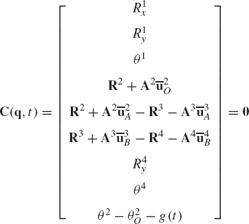
in which the first three constraints are the ground constraints, the fourth to the ninth constraints represented by the three vector equations are the revolute joint constraints, the tenth and eleventh constraints are the prismatic joint constraints, and the twelfth constraint is the driving constraint.
The Newton-Raphson iterative procedure used for the position analysis requires the evaluation of the constraint Jacobian matrix, which is defined for this example as
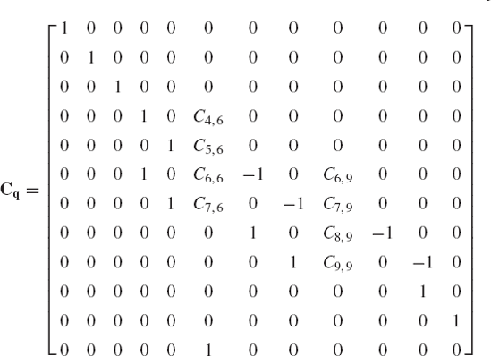
where
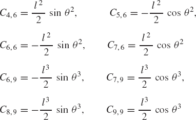
Using the Jacobian matrix and the vector of constraint equations, an iterative Newton-Raphson procedure can be used to determine the coordinates of the bodies of the slider crank mechanism. Figures 37a and 37b show, respectively, the angular orientation of the connecting rod and the displacement of the slider block as a function of the crank angle when the crankshaft rotates with a constant angular velocity equal to 150 rad/s. In this special case, g(t) = 150t.
For the velocity analysis, one needs to evaluate the vector Ct, which is given in this case by
where f(t) = 150. Figures Figure 38a and Figure 38b show, respectively, the angular velocity of the connecting rod and the velocity of the slider block as functions of the crank angle.
For the acceleration analysis, the Jacobian matrix and the vector Qd must be evaluated. The vector Qd is
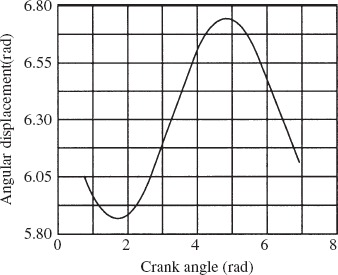
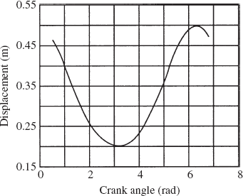
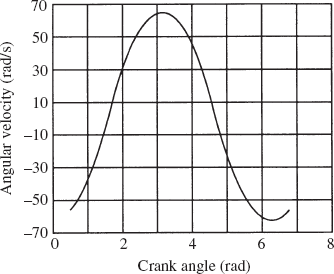
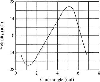
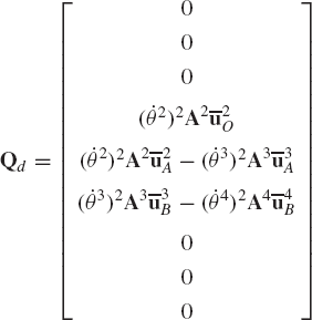
Using this vector and the Jacobian matrix, Eq. 137 can be solved for the accelerations. Figures Figure 39a and Figure 39b show, respectively, the angular acceleration of the connecting rod and the acceleration of the slider block as functions of the crank angle.
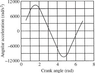
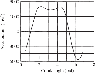
If the mechanism is kinematically driven by prescribing the motion of the slider block, the driving constraint in this case takes the following form:
where f(t) is a specified function of time. In this case, the vector of the constraint equations can be written as
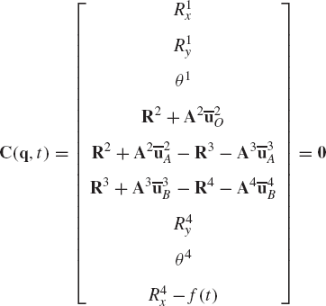
and the Jacobian matrix of the kinematic constraints is
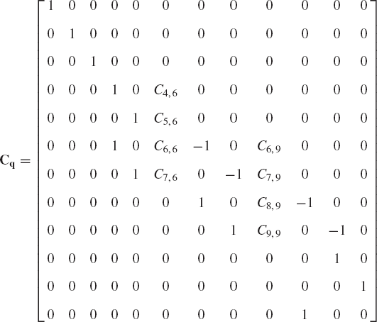
where the coefficients that appear in this matrix are the same as those defined in the case of the prescribed rotation of the crankshaft. The vectors Ct and Qd are
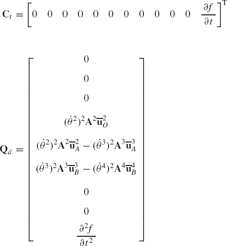
Figures 40a and 40b show, respectively, the angular orientations of the crankshaft and the connecting rod as functions of time when
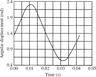
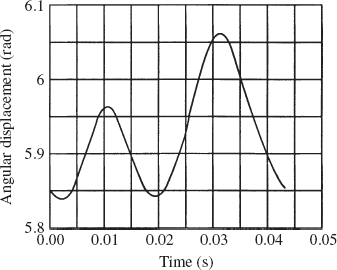
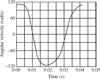
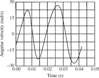
Figures 41a and 41b show, respectively, the angular velocities of the crankshaft and the connecting rod, while Figs. 42a and 42b show their angular accelerations as the result of the specified motion of the slider block.
At the special configuration in which θ2 = θ3 = 0, one has
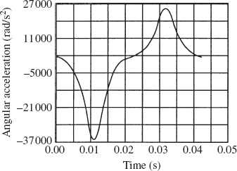
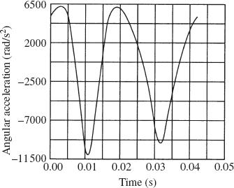
and at this special configuration, the Jacobian matrix becomes
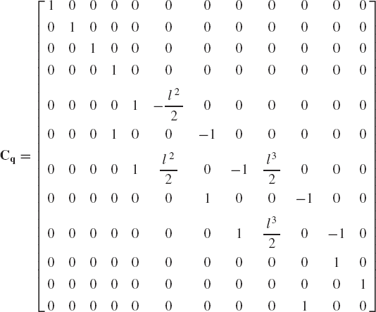
This matrix is singular since the sum of the sixth, eighth and twelfth rows is the fourth row. This is an indication that it is impossible to drive the mechanism at this singular configuration by specifying the motion of the slider block. This singularity, however, does not occur at this configuration when the mechanism is driven by specifying the angular orientation of the crankshaft.
In this chapter, methods for the analysis of kinematically driven systems are presented. Two distinctive, yet equivalent, procedures can be recognized from the kinematic development presented in this chapter. The first is the classical approach, which is suited for the analysis of multibody systems that consist of small numbers of bodies and joints. The kinematic analysis using the classical approach, as demonstrated by Examples 3 through 6, starts by developing trigonometric relationships between the angles that define the orientation of the bodies in the system. These trigonometric relationships, which depend on the topological structure of the system, define a set of nonlinear algebraic equations that can be solved for the position variables. Once the position coordinates are defined, the kinematic velocity analysis starts by considering the velocities of a body in the system and their relationships to the velocities of other bodies as the result of the joint connections. By utilizing the topological structure of a given system, a set of linear algebraic constraint equations in the velocities can be determined and solved for the time derivatives of the coordinates. The acceleration analysis can be performed once the velocities are determined, and in the classical approach it heavily utilizes the particular topological structure of the system, as in the case of the position and velocity analyses.
The second approach presented in this chapter is more general and can be applied to a wide class of multibody system applications. In this approach, the nonlinear constraint equations that describe mechanical joints and specified motion trajectories of the system are formulated. In the case of kinematically driven systems, the resulting number of equations is equal to the number of the system coordinates. Therefore, these equations can be solved using numerical and computer methods to determine the system coordinates. By differentiating the constraint equations once and twice with respect to time, one obtains linear systems of algebraic equations in the velocities and accelerations, respectively. These equations can be solved in a straightforward manner to determine the first and second time derivatives of the system coordinates. This procedure for the kinematic analysis can be implemented on the digital computer and used in the kinematic analysis of varieties of multibody system applications as demonstrated in this chapter.
In the analysis of kinematically driven systems, it is assumed that all the system degrees of freedom are specified. In this case, one obtains a number of algebraic equations equal to the number of system coordinates, and therefore, a complete kinematic analysis can be performed without the need for developing the differential dynamic equations of motion, which are expressed in terms of the inertia, applied, and/or joint forces. If one or more of the degrees of freedom are not specified, the algebraic constraint equations are not sufficient to solve for the system coordinates. This is the case of dynamically driven systems whose analysis requires use of the laws of motion and formulation of the differential equations of the system as well as consideration of the force relationships in addition to the kinematic relationships. In the following chapters, different techniques for formulating the dynamic equations of constrained multibody systems are presented and the computer implementation of these techniques is discussed.
Figure P1 shows a rigid body i that has a body fixed coordinate system XiYi. The global position vector of the origin of the body coordinate system Oi is defined by the vector Ri, and the orientation of the body i coordinate system in the global coordinate system is defined by the angle θi. The local position vector of point Pi on the body is defined by the vector

In problem 1, let

In the slider crank mechanism shown in Fig. P2, the lengths of the crankshaft OA and the connecting rod AB are, respectively, 0.3 and 0.5 m. The crankshaft is assumed to rotate with a constant angular velocity

Repeat problem 3 assuming that the offset h = 0.05;m.
The lengths of the crankshaft OA and the connecting rod AB of the slider crank mechanism shown in Fig. P2 are 0.3 and 0.5 m, respectively, and the offset h = 0.0. The motion of the crankshaft is such that θ2 = 150t + 3.0 rad. Determine the orientation of the connecting rod and the position of the slider block at time t = 0, 0.01, and 0.03 s.
The lengths of the crankshaft OA, coupler AB, and rocker BC of the four-bar linkage shown in Fig. P3 are, respectively, 0.3, 0.35, and 0.4 m. The distance OC is 0.32 m. The crankshaft rotates with a constant angular velocity of 100 rad/s. Determine the orientation and angular velocity and acceleration of the coupler and the rocker when the orientation of the crankshaft θ2 = 60°. Also determine the orientation and angular velocity and angular acceleration of the crankshaft and the coupler when the orientation of the rocker θ4 = 60°.
Using Eq. 29, show that the velocities of two points A and B on a rigid body have equal components along the line AB.
Repeat problem 1 assuming that the absolute velocity of the reference point is zero. Prove in this case, by using vector algebra, that the absolute velocity of point Pi is perpendicular to the line OiPi, where Oi is the reference point.
Show that in the case of a general rigid body displacement, there exists a point on the rigid body whose velocity is instantaneously equal to zero. This point is called the instantaneous center of rotation.
In problem 3, let the velocity of the slider block be constant and equal to 5 m/s. Determine the angular velocities and angular accelerations of the crankshaft and the connecting rod. Also determine the absolute velocity and acceleration of the center of the connecting rod.
Prove the identities of Eq. 35.
Prove the identity of Eq. 49.
The motion of a rigid body i is such that the location of the origin of its reference is defined by the vector
Solve problem 13 assuming that
Examine the singular configurations of the four-bar mechanism.
In the system shown in Fig. P4, OA = 0.2;m, OB = 0.3;m, and BC = 0.6;m. Link OA is assumed to rotate with an angular velocity 50 rpm counter-clockwise. Find the velocity and acceleration of point C and the angular velocity and acceleration of link BC.
Figure P5 shows a gear system that consists of gears i, j, and k, which are pinned at their centers to the rod r at points O, A, and B, respectively. Gear i is fixed with ri = 0.3;m, while rj = rk = 0.1;m. If the rod r rotates counterclockwise with a constant angular velocity of 15 rad/s, determine the angular velocities and angular accelerations of the gears j and k.
Solve problem 17 if the angular velocity and the angular acceleration of the rod are 15 rad/s, and 120 rad/s2, respectively. The angular velocity and acceleration of the rod are assumed to be counterclockwise.
The motion of a rigid body i is such that the global coordinates of point P on the rigid body is given by
The motion of two bodies i and j is such that Rix = 5 m = constant, Riy = 3sin5t;m,

where
Derive the vector of the constraint equations of this system and determine the number of degrees of freedom.
For the three-body system shown in Fig. P6, use three absolute coordinates for each body to write the kinematic constraint equations of the revolute and prismatic joints. Also derive the constraint Jacobian matrix for the system.
Figure P7 shows two bodies i and j connected by a revolute-revolute joint that keeps the distance between points Pi and Pj constant. Derive the constraint equations for this type of joint using the absolute Cartesian coordinates. Derive also the constraint Jacobian matrix for this joint.
Derive the constraint Jacobian matrix of the reciprocating knife-edge follower cam system, and the roller follower cam system.
Derive the kinematic constraint Jacobian matrix of the offset flat-faced follower of Example 8.
Determine the vectors Ct and Qd of Eqs. 121 and 124, respectively, for the revolute-revolute joint of problem 22.
Determine the vectors Ct and Qd of Eqs. 121 and 124, respectively, in the case of the reciprocating knife-edge follower cam system and the roller follower cam system of problem 23.
Determine the vectors Ct and Qd of Eqs. 121 and 124, respectively, in the case of the offset flat-faced follower of Example 8.
Derive the constraint equations, the Jacobian matrix, the vector Ct, and the vector Qd for the system shown in Fig. P8 using the absolute Cartesian coordinates.
Figure P9 shows a slider crank mechanism. The lengths of the crankshaft and the connecting rod are 0.2 m and 0.4 m, respectively. The crankshaft is assumed to rotate with a constant angular velocity
Figure P10 shows a four-bar mechanism. The lengths of the crankshaft, coupler, and rocker are 0.2 m, 0.4 m, and 0.3 m, respectively. The crankshaft of the mechanism is assumed to rotate with a constant angular velocity