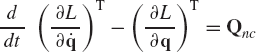
The principle of virtual work represents a powerful tool for deriving the static and dynamic equations of multibody systems. Unlike Newtonian mechanics, the principle of virtual work does not require considering the constraint forces, and it requires only scalar work quantities to define the static and dynamic equations. This principle can be used to systematically derive a minimum set of equations of motion of the multibody systems by eliminating the constraint forces. To use the principle of virtual work, the important concepts of the virtual displacements and generalized forces are first introduced and used to formulate the generalized forces of several force elements, such as springs and dampers and friction forces. It is shown in this chapter that the principle of virtual work can be used to obtain a number of equations equal to the number of the system degrees of freedom, thereby providing a systematic procedure for obtaining the embedding form of the equations of motion of the mechanical system. Use of the principle of virtual work in statics and dynamics is demonstrated using several applications. The principle of virtual work is also used in this chapter to derive the well-known Lagrange's equation, in which the generalized inertia force is expressed in terms of the scalar kinetic energy. Several other forms of the generalized inertia forces are also presented, including the form that appears in the Gibbs-Appel equation, in which the generalized inertia is expressed in terms of an acceleration function. The Hamiltonian formulation and the relationship between the virtual work and the Gaussian elimination are discussed in the last two sections of this chapter.
An important step in the application of the principle of virtual work is the definition of the virtual displacements and generalized forces. The concept of the generalized forces is introduced in Section 3, while the concept of the virtual displacement is discussed in this and the following section. Throughout this section and the sections that follow, the term generalized coordinates is used to refer to any set of coordinates used to describe the system configuration.
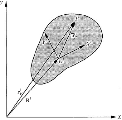
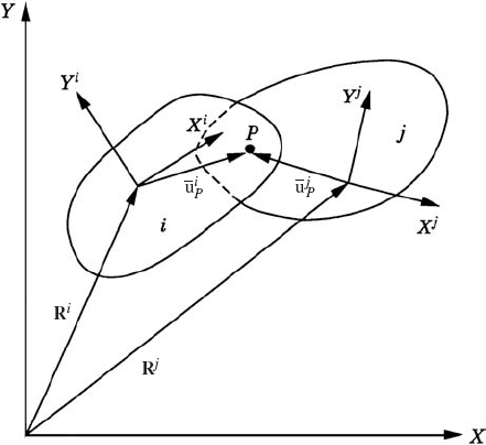
The virtual displacement is defined to be an infinitesimal displacement that is consistent with the kinematic constraints imposed on the motion of the system. Virtual displacements are imaginary in the sense that they are assumed to occur while time is held fixed. Consider, for instance, the displacement of the unconstrained body shown in Fig. 1. The position vector of an arbitrary point Pi on the rigid body is given by
where Ri is the position vector of the reference point,
where θi is the angle that defines the orientation of the body. A virtual change in the position vector of point Pi of Eq. 1 is denoted as δriP and is given by
Since the vector
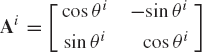
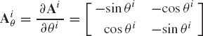
where Aiθ is the partial derivative of Ai with respect to the angle θi, that is,
In Eq. 4, the virtual change in the position vector of an arbitrary point on the body is expressed in terms of the virtual changes in the body coordinates, or in this case the body degrees of freedom. Equation 4 can also be written as
where
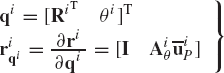
Clearly, if the reference point Oi is fixed, as in the case of a simple pendulum, we have δRi = 0 and Eq. 4 reduces to
Example 5.1
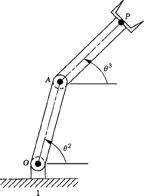
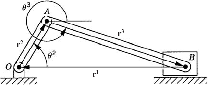
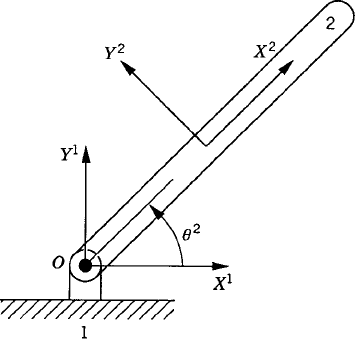
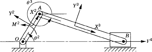
For the two-degree-of-freedom manipulator shown in Fig. 2, express the virtual change in the position of point P (end effector) in terms of the virtual changes in the system degrees of freedom.
Solution. The position vector of point P is given by
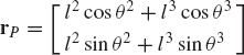
where l2 and l3 are, respectively, the lengths of links 2 and 3 (the fixed link is denoted as body 1), and θ2 and θ3 are, respectively, the angular orientations of links 2 and 3. By taking a virtual change in the position vector of point P, we obtain
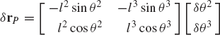
which can be written as
Virtual displacements can be regarded as partial differentials with time assumed to be fixed. Thus, the differential of time is taken to be zero. To explain the difference between the actual displacement and the virtual displacement, we consider the case of a position vector that is an explicit function of the generalized coordinates q and time t. This vector can be written as
Differentiating this equation with respect to time, one obtains
Multiplying both sides of this equation by dt yields the actual differential displacement as
If r is not an explicit function of time, the virtual displacement δr and the actual differential displacement dr are the same provided that the partial differential δq is the same as the total differential dq. It follows that in the case of an n-dimensional vector of generalized coordinates, one has
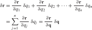
where qj is the jth generalized coordinate, and
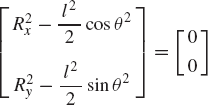
In constrained multibody systems, the system coordinates are related by a set of kinematic constraint equations as the result of mechanical joints or specified motion trajectories. If the system is not kinematically driven, the number of the kinematic constraint equations nc is less than the number of the system coordinates n. In this case, the constraint kinematic relationships can be used to write a subset of the coordinates in terms of the others. Therefore, the coordinates of a multibody system can be divided into two groups: the first group is the set of dependent coordinates qd and the second group is the set of independent coordinates or the degrees of freedom of the system qi. The number of dependent coordinates is equal to the number of the kinematic constraint equations nc and the number of independent coordinates is equal to n − nc. By using the kinematic relationships, the virtual changes in the dependent coordinates can be expressed in terms of the virtual changes of the independent coordinates. Consider, for example, the slider crank mechanism shown in Fig. 3. The loop-closure equations for this mechanism can be written in a vector form as
which can be written more explicitly as
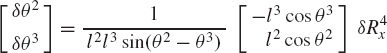
where l2 and l3 are the lengths of the crankshaft and the connecting rod, and R4x is the position of the slider block with respect to point O. By taking the virtual changes of the coordinates, the preceding equation leads to
One may select the dependent coordinates to be θ3 and R4x, that is,
where qd is the nc-dimensional vector of dependent coordinates. Since the mechanism has only one degree of freedom, there is only one independent coordinate that can be selected as θ2, that is, qi=θ2. One may then rearrange Eq. 14 and write this equation using matrix notation as
which defines δθ3 and δR4x in terms of the independent coordinate δθ2 as
It is clear from this equation that a singular configuration occurs when θ3 = π/2 or 3π/2. At this singular configuration δθ3 and δR4x cannot be expressed in terms of δθ2.
Alternatively, one may try to express δθ2 and δθ3 in terms of δR4x using Eq. 14. This leads to
The solution of this matrix equation is
In this case, singularity occurs whenever θ2 is equal to θ3.
Example 5.2
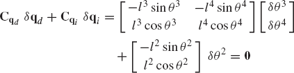
For the four-bar linkage shown in Fig. 4, obtain an expression for the virtual changes in the angular orientations of the coupler and the rocker in terms of the virtual change of the angular orientation of the crankshaft.
Solution. The loop-closure equations for this mechanism are
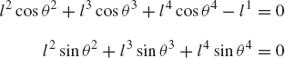
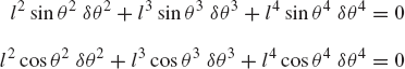
where l2, l3, and l4 are, respectively, the lengths of the crankshaft, coupler, and rocker; l1 is the distance between points O and C; and θ2, θ3, and θ4 are, respectively, the angular orientations of the crankshaft, coupler, and rocker. By taking virtual changes in the coordinates θ2, θ3, and θ4, and keeping in mind that l1 is constant, the loop-closure equations yield
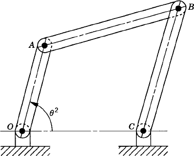
The coordinates θ3 and θ4 may be selected as dependent coordinates and θ2 as the independent coordinate leading to the following relationship:
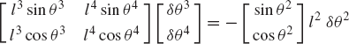
or
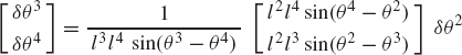
A similar procedure can be used if δθ3 or δθ4 is selected to be the independent coordinate.
One may generalize the procedure described in this section for expressing the virtual changes of the dependent coordinates in terms of the virtual changes of the independent ones. This can be demonstrated by writing the algebraic kinematic constraint equations between coordinates in the following general form:
where q = [q1 q2 ... qn]T is the vector of the system coordinates, t is time, and C is the vector of constraint functions, which can be written as
where nc is the total number of constraint equations that are assumed to be linearly independent. If the system is dynamically driven, the number of constraint equations nc is less than the number of the coordinates n.
Equation 20, as the result of a virtual change in the vector of system coordinates, leads to
where Cq is the constraint Jacobian matrix defined as
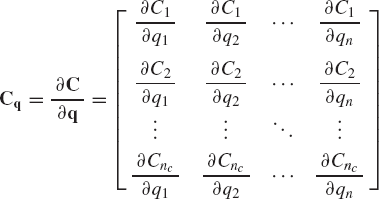
The constraint Jacobian matrix has a number of rows equal to the number of constraint equations and a number of columns equal to the number of the system coordinates. The vector of coordinates q can be written in the following partitioned form:
where qd is an nc-dimensional vector of the dependent coordinates, and qi is an (n − nc)-dimensional vector of independent coordinates. According to this coordinate partitioning, Eq. 22 can be rewritten as
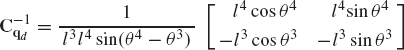
where the dependent and independent coordinates are chosen such that the nc × nc matrix is nonsingular. Equation 25 can then be used to write δqd in terms of δqi as
or simply as
where
By using Eqs. 24 and 27, the virtual change in the total vector of system coordinates can be expressed in terms of the virtual change of the independent coordinates as
This equation can be written as
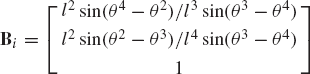
where the matrix Bi is an n × (n − nc) matrix defined as
Example 5.3
The use of the general procedure described in this section can be demonstrated using the four-bar linkage discussed in Example 2. In this example, the vector of coordinates q is selected to be
The kinematic constraint equations that relate these coordinates are defined by the loop-closure equations of Example 2. These constraint equations are
By taking a virtual change in the system coordinates, one has
which can also be written as
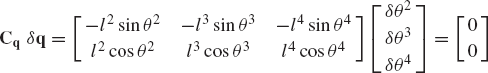
From which the Jacobian matrix of the kinematic constraints can be identified as
If θ2 is selected as the independent coordinate, one has
It follows that
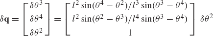
The virtual changes in the dependent coordinates can then be expressed in terms of the virtual change in the independent coordinate as
Since in this example
the preceding equation yields
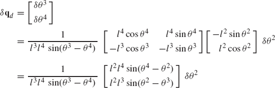
which is the same result obtained in Example 2. The matrix Cdi of Eq. 28 is recognized as
The virtual change in the total vector of system coordinates can be expressed in terms of the virtual change in the independent coordinate as
where the matrix Bi of Eq. 31 can be recognized as
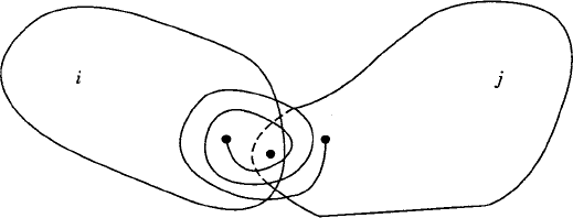
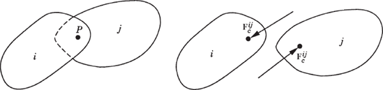
As pointed out in Chapter 3, in many general-purpose multibody computer algorithms the absolute coordinates are employed for the sake of generality. In this case, the configuration of the rigid body is identified by the global position vector of the origin of the body reference (reference point) and by a set of orientational coordinates that define the orientation of the body in a global fixed frame of reference. Kinematic constraints that represent mechanical joints in the system can be formulated in terms of the absolute coordinates. For example, the algebraic kinematic constraint equations that describe the revolute joint between body i and body j in Fig. 5 can be expressed as
where riP is the position vector of the joint definition point P expressed in terms of the coordinates of body i, and rjP is the position vector of the same point P expressed in terms of the coordinates of body j. Equation 32 can be written in a more explicit form in terms of the absolute coordinates as
where Ri and Rj are, respectively, the position vectors of the reference points of body i and body j, Ai and Aj are the transformation matrices of body i and body j, and
By taking a virtual change in the absolute coordinates of body i and body j, Eq. 33 leads to
Since the revolute joint eliminates two degrees of freedom, one may select δRj as the vector of dependent coordinates and write this vector in terms of the other absolute coordinates as
Example 5.4
Figure 6 shows a two-body system that consists of the ground and a rigid rod with a uniform cross-sectional area and length l2. In this example, three absolute coordinates Rix, Riy, and θi are selected for each body i in the system. The reference point of the rod is assumed to be at its geometric center. If the system is assumed to be dynamically driven, there are only joint constraints that represent the ground and the revolute joint constraints. The ground constraints are
The revolute joint constraints are
where
The vector of the system generalized coordinates is
The vector of the system constraint equations is
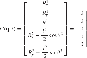
and the constraint Jacobian matrix is
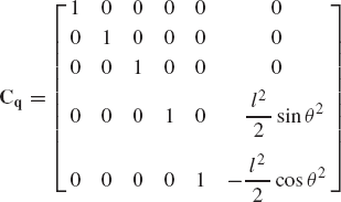
In this example, there are six coordinates (n = 6) and five constraint equations (nc = 5). Therefore, the system has one degree of freedom. One may select this degree of freedom to be θ2 and write Eq. 25 as
where in this case qd = [R1x R1y θ1 R2x R2y]T and qi = θ2. According to this generalized coordinate partitioning, the matrices Cqd and Cqi can be identified as
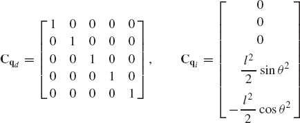
It follows that the matrix Cdi of Eq. 28 can be written in this case as
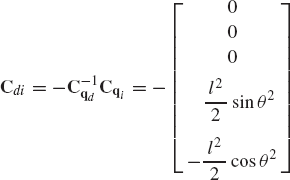
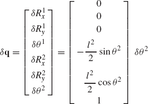
and the matrix Bi in Eq. 30 is
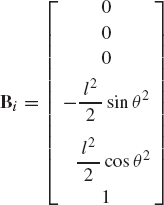
Using Eq. 30, the virtual change in the total vector of the system coordinates can be expressed in terms of the virtual change in the system degrees of freedom as
Joint and driving constraints that can be described by Eq. 20 are called holonomic constraints since they can be expressed as algebraic equations in the system coordinates and time. There are other types of constraints that cannot be expressed as functions of the coordinates and time only. These types of constraints, which are known as nonholonomic constraints, can be expressed in terms of differentials of the coordinates as
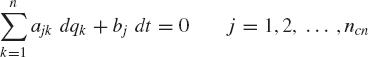
where ncn is the number of nonholonomic constraint equations, and ajk and bk can be functions of the system coordinates q = [q1 q2 ... qn]T as well as time. One should not be able to integrate the preceding equation and write it in terms of the coordinates and time only; otherwise we obtain the form of the holonomic constraints. Hence, one cannot use nonholonomic constraints to eliminate dependent coordinates and, consequently, in this case of a nonholonomic system, the number of independent coordinates is more than the number of independent velocities.
Recall that a differential form is integrable if it is an exact differential. In this case, the following conditions hold:
If these conditions are not satisfied, Eq. 36 is of the nonholonomic type since this equation cannot be integrated and written in the form of Eq. 20. It follows that in the case of a nonholonomic system, none of the constraint equations of Eq. 36 can be written in the form
An example of nonholonomic constraints is
These are two independent constraint equations expressed in terms of the differentials of the four coordinates q1, q2, q3, and q4. These two equations do not satisfy the conditions of exact differentials of Eq. 37, and therefore, they cannot be integrated and expressed in the form of Eq. 20.
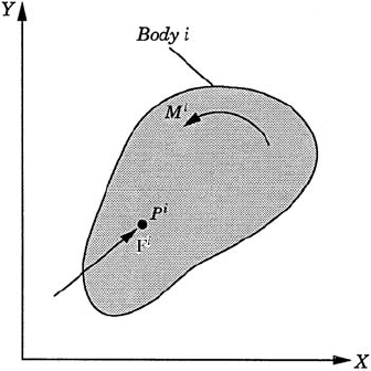
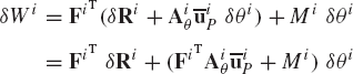
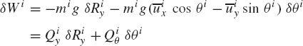
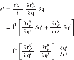
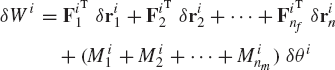
The virtual work of a force vector is defined to be the dot (scalar) product of the force vector and the vector of the virtual change of the position vector of the point of application of the force. Both vectors must be defined in the same coordinate system. The virtual work of a moment that acts on a rigid body is defined to be the product of the moment and the virtual change in the angular orientation of the body. Figure 7 shows a rigid body i that is acted upon by a moment Mi and a force vector Fi whose point of application is denoted as Pi. The virtual work of this system of forces is given by
where riP is the position vector of point Pi, and θi is the angular orientation of the body i.
The position vector of an arbitrary point on a rigid body can be expressed in terms of the position vector of the reference point as well as the angular orientation of the body. The coordinates of the rigid body may be defined by the vector qi where
where Ri is the position vector of the reference point and θi is the angular orientation of the body. In terms of these coordinates, the position of point Pi given by the vector riP of Eq. 40 can be written as
where Ai is the transformation matrix from the body coordinate system to the global coordinate system, and
Substituting Eq. 43 into Eq. 40, the virtual work of the force Fi and the moment Mi can be expressed as
This equation can be written as
where
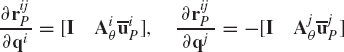
The vector QiR is called the vector of generalized forces associated with the coordinates of the reference point, and the scalar Qiθ is called the generalized force associated with the rotation of the body. The second term in the second equation of 46, which is the contribution of the force Fi to the generalized force associated with the rotation of the body, can be written as
One can verify that this equation also takes the following form:
or
where k is a unit vector along the Z axis, and
Equations 46 and 50 imply that a force vector Fi that acts at an arbitrary point Pi is equivalent (equipollent) to another system of forces that consists of the same force Fi acting at the reference point and a moment (uip×Fi). k associated with the rotation of the body.
The method discussed in this section for obtaining the generalized forces can be generalized to any number of forces and moments. The procedure is to express the position vectors of the points of application of the forces in terms of the system coordinates. Substituting the resulting kinematic relationships into the expression for the virtual work leads to the definition of the generalized forces associated with the system coordinates. For example, if the configuration of the multibody system is described by the n coordinates
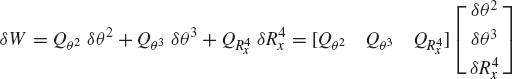
The virtual work of the forces acting on the system can be expressed in the general form
where Qj is the generalized force associated with the jth coordinate qj.
Equation 52 can be written in a vector form as
where Q is the vector of generalized forces and δq is the vector of the virtual changes in the coordinates. The vectors Q and δq are
Equation 52 or its equivalent vector form of Eq. 53 defines the generalized forces associated with the coordinates q = [q1 q2...qn]T. The generalized forces associated with another set of coordinates can be obtained if the transformation between the two sets of coordinates is defined. Let p = [p1 p2...pm]T be another set of coordinates such that the vector of virtual changes in q can be expressed in terms of the virtual changes in p as
By substituting Eq. 55 into Eq. 53, one obtains
where
is the vector of generalized forces associated with the vector of coordinates p.
Example 5.5
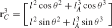
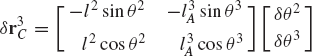
As an illustrative example, the slider crank mechanism shown in Fig. 8 is considered. The virtual work of the external forces acting on the links of this mechanism is
where F3 = [F3x F3y]T. The vector r3C is
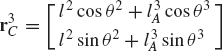
where l3A is the distance between points A and C. Therefore, one has
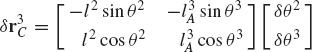
Substituting this equation into the expression for the virtual work, one obtains

or
where
It was shown in Section 2 that δθ3 and δR4x can be expressed in terms of δθ2 as
One may define the vector q as
The virtual change in this vector can be written in terms of the virtual change in θ2 as
Substituting this equation into the expression of δW leads to the definition of the generalized force, of all the forces and moments acting on the slider crank mechanism, associated with the coordinate θ2 as
where in this case δp reduces to δp = δθ2, and
in which
Example 5.6
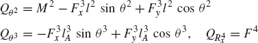
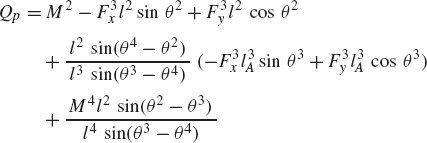
Determine the generalized force associated with the rotation of the crank shaft, due to the system of forces acting on the four-bar linkage shown in Fig. 9.
Solution. The virtual work of the forces shown in Fig. 9 is given by
where F3 = [F3x F3y]T and
where l3A is the distance between point A and the center of the coupler. It follows that
Substituting this into the expression for the virtual work, one obtains
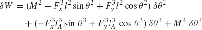
By using the results of Example 2, δθ3 and δθ4 can be expressed in terms of δθ2 as
which upon substitution into the expression of the virtual work yields
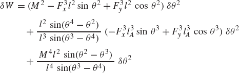
where
Before concluding this section it is important to point out that, in general, the virtual work is not an exact differential. That is, the virtual work is not, in general, the variation of a certain function. In the special case where the virtual work is an exact differential one has
and consequently,
In this special case, the forces are said to be conservative since they can be obtained using a potential function. Nonconservative forces, however, cannot be derived from a potential function, and hence their virtual work is not equal to the variation of a certain function. Examples of conservative forces are the gravity forces and linear spring forces. Examples of nonconservative forces are the damping, friction, and actuator forces. In this book, for the sake of generality, we use the general expression of Eq. 53 to define the generalized forces regardless of whether these forces are conservative or nonconservative.
In this section, the generalized forces associated with some of the commonly encountered forces in multibody dynamics are developed. The definitions of these generalized forces are obtained by using the virtual work expression.
The virtual work of the gravity force acting on body i is given by
where mi is the mass of body i, g is the gravity constant, and yi is the vertical coordinate of the position vector of the body center of mass. If the reference point is the same as the center of mass, one has δyi = δRiy. If, on the other hand, the reference point is different from the center of mass, yi can be expressed in terms of the coordinates of body i as
where
which upon substitution into the expression for the virtual work of Eq. 60 leads to
where Qiy and Qiθ are, respectively, the generalized forces associated with the coordinates Riy and θi, and are given by
If the reference point is selected to be the center of mass of the body, Qiθ is identically zero since
Figure 10 shows two bodies i and j connected by a force element that consists of a translational spring, damper, and actuator. The spring stiffness is assumed to be k, the damping coefficient is C, and the actuator force is fa. The point of attachment of this force element on body i is assumed to be Pi, while on body j it is assumed to be Pj. The position vectors of these points with respect to their respective body coordinate systems are denoted as
where l is the current spring length, l0 is the undeformed length of the spring, and
The virtual work due to the force defined by Eq. 65 can be written as
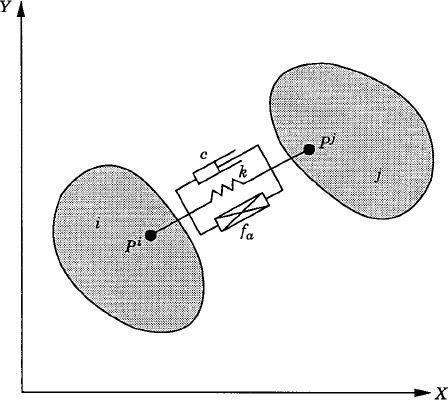
where δl is the virtual change in the distance between points Pi and Pj. In terms of the absolute coordinates of the two bodies, the position vector of point Pj with respect to point Pi can be written as
One can, therefore, define the current spring length as
and the virtual change in this length as
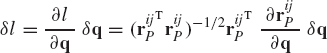
where q is the vector of coordinates of body i and body j given by
Equation 69, upon the use of Eq. 68, can be expressed as
where
The generalized forces associated with the coordinates of body i and body j can be obtained by substituting Eq. 71 into Eq. 66, yielding
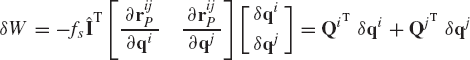
where Qi and Qj are the vectors of the generalized forces associated with the coordinates of body i and body j, respectively. Using Eq. 72, these vectors are
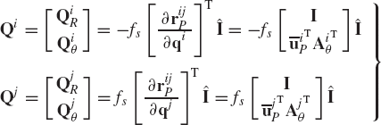
in which fs is defined by Eq. 65. In the expression for the force fs, l is defined by Eq. 68, and
The special case, in which there is only a spring element, can be obtained from the general development presented in this section by assuming that c = fa = 0. Similarly, if the force element consists of a damper or an actuator only, one has k = fa = 0 or k = c = 0, respectively.
Example 5.7
Figure 11 shows a spring-damper force element that is connected between the crankshaft and the rocker of a four-bar linkage. The stiffness coefficient k of the spring is assumed to be 250 N/m and the damping coefficient C is assumed to be 10 N · s/m. The undeformed length of the spring is assumed to be 0.35 m. The local positions of the attachment points of the spring-damper element with respect to the crankshaft and the rocker coordinate systems are given, respectively, by
Solution. By performing a position analysis for the four-bar mechanism, one obtains
The velocity analysis leads to
The spring-damper force is
The virtual work of the spring-damper force is
Note that
It follows that
A unit vector along a line connecting the attachment points of the spring-damper element is
The vector of the generalized coordinates of the crankshaft and the rocker can be written as
The time derivative of the spring length is
in which
which yield
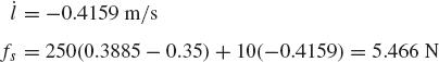
The generalized forces can then be written as
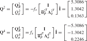
These are the generalized forces associated with the absolute coordinates of the crankshaft and the rocker. Note that the forces associated with the translational coordinates are equal in magnitude and opposite in direction.
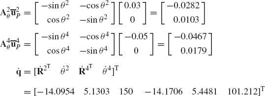
To determine the generalized forces associated with the angles θ2, θ3, and θ4, we first evaluate δr24P as
where
and
Using this equation, it can be shown that
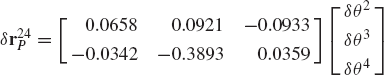
The spring-damper force vector is
The virtual work of this force is
where the generalized forces associated with the angles θ2, θ3, and θ4 are recognized as
Figure 12 depicts two bodies i and j that are connected by rotational spring and damper. The stiffness coefficient of the spring is assumed to be kr and the damping coefficient is assumed to be cr. The resultant moment of the spring and damper can be expressed as
where θ0 is the angle between body i and body j before displacements, and θ is the relative angular displacement between the two bodies, that is, θ = θi − θj. The virtual work due to the moment of Eq. 76 is
Using the preceding two equations,
where Qiθ and Qjθ are the generalized forces associated with the rotational coordinates of bodies i and j, respectively. These generalized forces are
If the force element consists of a spring only, cr=0. On the other hand, if the force element consists of a damper only, kr = 0
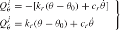
In the case of ideal joints, the reaction forces are assumed to be normal to the contact surfaces. Although this assumption is valid in many situations and its use leads to a relatively small error, there are many applications wherein the interaction between the contact surfaces must be described by normal and tangential components. The tangential component that opposes the relative motion between the two surfaces is called the friction force. In many types of multibody systems, such as gears and bearings, it is desirable to minimize the effect of the friction forces, while in other applications, such as brakes and clutches, one desires to maximize the friction effect.
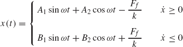
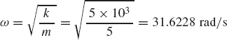
In the case of Coulomb or dry friction, the friction force is not an explicit function of the displacement and its derivatives. Figure 13a shows two bodies i and j that are in contact. Let t be a unit vector along the flat contact surface, and vi and vj be the absolute velocities of the reference points of the two bodies. The velocity of body i with respect to body j along the vector t is
Table 5.1. Coefficient of Statis Friction
Rubber on concrete | 0.60–0.90 |
Metal on stone | 0.30–0.70 |
Metal on wood | 0.20–0.60 |
Metal on metal | 0.15–0.60 |
Metal on metal | 0.15–0.60 |
Stone on stone | 0.40–0.70 |
As shown in Fig. 13a, the contact force is represented by two components; the component Fn, which is normal to the flat contact surface, and the component Ff, which is parallel to that surface. The component Ff, which is developed by friction, opposes the relative motion. In the classical theory of dry friction, the friction force Ff is directly proportional to the normal force Fn. Depending on the materials of the two bodies, there is a limit to the magnitude of the force Ff. In the special case where vr=0, one has
where μs, called the coefficient of static friction, depends on the properties of the materials in contact. The values of the coefficient of static friction can be found experimentally. Table 1 shows approximate values of this coefficient in several cases of dry surfaces.
If body i slides with respect to body j with a relative velocity vr, the friction force takes on the value
where μk is called the coefficient of sliding friction. This coefficient can also be determined experimentally and its value is slightly less than μs for most materials. The function sgn(vr) has the value ±1 depending on the sign of its argument vr. Figure 13b shows the friction force Ff as a function of the relative velocity vr. It is clear from this figure that when vr is equal to zero, the friction force Ff can have any magnitude. The actual magnitude of this force can be determined from the static equilibrium conditions. While it is often assumed in the analysis of systems involving dry friction that the maximum friction force is μkFn, in reality the force required to initiate the motion is slightly larger than the force required to maintain it.
It is clear from Eq. 83 that
where the angle ϕ shown in Fig. 13a is called the friction angle.
Example 5.8
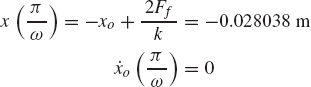
The mass-spring system shown in Fig. 14 has mass m = 5 kg, stiffness coefficient k = 5 × 10³ N/m, coefficient of friction μk = 0.1, initial displacement xo = 0.03 m, and zero initial velocity. Determine the number of cycles of oscillations of the mass before it comes to rest.
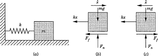
Solution. The equation of motion of the mass is
where the negative sign is used when the mass moves to the right and the positive sign is used when the mass moves to the left. The solution of the differential equation of motion can be written as
where ω is the natural frequency of the system defined as
Substituting with the initial conditions into Eq. 85b, which describes the dynamics of the system when the mass moves to the left, one obtains
where
It follows that
Therefore, the displacement and velocity of the mass when it first moves to the left can be described by the equations
The direction of the motion will change when the velocity is equal to zero, that is
which yields
At this time the displacement is determined from Eq. 85b, which describes the motion to the left, as
This equation shows that the amplitude in the first half cycle is reduced by the amount 2Ff/k as the result of dry friction.
In the second half cycle, the mass moves to the right and the motion is governed by Eq. 85a, which describes the motion to the right with the initial conditions
These initial conditions yield
The displacement x(t) in the second half cycle can then be written as
and the velocity
The velocity is zero at time t2=2π/ω=τ, where τ is the periodic time of the natural oscillations. At time t2, the end of the first cycle, the displacement is
which indicates that the amplitude decreases in the second half cycle by the amount 2Ff/k, as shown in Fig. 15. By continuing in this manner, one can verify that there is a constant decrease in the amplitude of 2Ff/k every half cycle. It is not necessary that the system comes to rest at the undeformed spring position. The final position will be at an amplitude Xf, where the spring force Fs = kXf is less than or equal to the friction force. In this example, the motion will stop if
or
The amplitude loss per half cycle is
The number of half cycles nr completed before the mass comes to rest can be obtained from the following equation:
which implies that
The smallest nr that satisfies this inequality is nr = 15 half cycles; that is, the number of cycles completed before the mass comes to rest is 7.5.
The preceding example demonstrates the complexity of the analysis of dry friction using a simple mass spring system. In a more complex mechanical system that consists of a set of interconnected bodies, the generalized friction forces associated with the system generalized coordinates can be systematically determined. Recall that in rigid body dynamics, a force is a sliding vector that can be moved along its line of action without changing its effect. It follows that once the friction force along the flat contact surface is determined, the generalized forces associated with the generalized coordinates of two bodies i and j in contact can be simply obtained using the concept of equipollent systems of forces or using the expression of the virtual work of the friction force where the point of application of the force is assumed to be an arbitrary point on the contact surface.
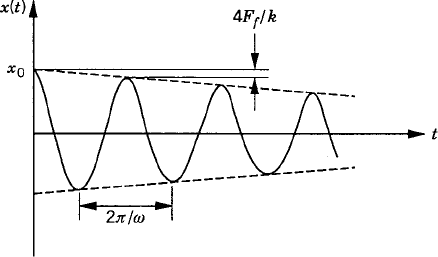
Further generalization of the development presented in this section can be made if the friction force is considered as arising from uniformly or nonuniformly distributed shear stress at the contact area (Greenwood, 1988). In this case, the frictional shear stress is equal to μk times the normal pressure. While this approach gives the same results for the simpler case of a flat contact surface, it can also be used in the analysis of more complicated systems. In order to demonstrate the use of this approach, consider the case of a circular rotating disk of radius a being pressed against another disk with a force Fn. If the compressive stress σn is assumed to be uniform, one has
The moment due to the friction force acting on an annular element of radius dr and area dA = 2πr dr as shown in Fig. 16 is
which upon integration leads to
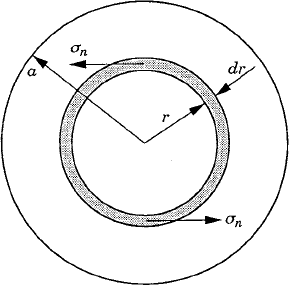
Another important friction application pertains to wheeled vehicles, which depend on the friction forces for starting, moving, and stopping. A point on a moving wheel as the one shown in Fig. 17 can have an instantaneous zero velocity while its acceleration is different from zero. Generally, there are two different situations that may occur. In the first situation, the wheel rolls and slides on the ground such that the wheel motion can be described using two degrees of freedom; one describes the rolling motion, while the other describes the sliding displacement. Because of the sliding motion, the velocity of the point of contact P on the wheel is not equal to zero. In the case of pure rolling motion, on the other hand, no sliding occurs and the instantaneous velocity of the contact point P on the wheel is equal to zero. In this case, the instantaneous velocity of the center of the wheel C is
where ω is the angular velocity of the wheel, and uCP is the position vector of point C with respect to point P. We must keep in mind that while in the preceding equation the velocity of point C is obtained using the instantaneous velocity of point P, vC takes on the same value so long as uCP represents the position vector of point C with respect to the contact point P. The direction of this velocity is always perpendicular to CP and its magnitude is equal to
where α is the angular acceleration of the wheel. The absolute acceleration of the contact point P can then be written as
Assuming that the wheel is balanced such that its center of mass is the same as its geometric center, the absolute acceleration of the center of mass is equal to aC. Since in the case of pure rolling the wheel has only one degree of freedom, the equation of motion of the wheel can be obtained by taking the moments of the inertia and applied forces about the contact point P. This equation can be used to determine the unknown force or acceleration. The reaction force at the contact point can then be determined by evaluating the sum of the forces in the vertical direction.
Mechanical joints in multibody systems give rise to constraint forces that influence the motion of the system components. These forces appear in the static and dynamic equations when the equilibrium conditions are developed for each body in the system. As demonstrated in the remainder of this book, the resulting system of equations can be solved for a number of unknowns equal to the number of the constraint reaction forces plus the number of the system degrees of freedom. These equations, by eliminating the reaction forces, reduce to a number of equations equal to the number of degrees of freedom of the system, and therefore, the constraint reaction forces may be considered as auxiliary quantities that we are forced to introduce when we study the equilibrium of each body in the system separately. These forces, which can be eliminated by considering the equilibrium of the entire system of bodies, are the result of workless or ideal constraints. The internal reaction forces between the particles that form a rigid body are constraint forces which do no work. This can be demonstrated by using the fact that the distance between two particles i and j on a rigid body remains constant, that is,
where ri and rj are, respectively, the position vectors of the particles i and j, and c1 is a constant. By assuming a virtual change in the position vector of the two particles, Eq. 92 yields
Let Fijc be the constraint force acting on particle i as the result of the kinematic constraint of Eq. 93. Newton's third law states that when two particles exert forces on each other, the resulting interaction forces are equal in magnitude, opposite in direction, and directed along the straight line joining the two particles. According to this law, one may write Fjic = − Fijc as the reaction force that acts on particle j. Furthermore,
where c2 is a constant. The virtual work of the forces Fijc and Fjic can be written as
Substituting Eq. 94 into Eq. 95 and using Eq. 93, yields
which implies that the connection forces resulting from the constraints between the particles forming the rigid body do no work.
Similar comments apply to the case of other friction-free mechanical joints such as the revolute joint shown in Fig. 18. For instance, the virtual work of the reaction forces acting on body i is
where rP is the global position vector of the joint definition point P shown in Fig. 18. The virtual work of the joint reaction forces acting on body j is
Using the preceding two equations, one has
This simple fact will be utilized in developing the principle of virtual work to eliminate the reaction forces from the equilibrium conditions leading to a number of equations equal to the number of degrees of freedom of the system.
The concepts and definitions presented in the preceding sections are used in this section to develop the principle of virtual work for static equilibrium. The principle of virtual work in dynamics is discussed in the following section.
The first step in deriving the principle of virtual work is to prove that two equipollent systems of forces produce the same virtual work. It was shown in Section 3 that a force Fi acting at an arbitrary point Pi on a rigid body i is equipollent to a force Fi that acts at the reference point and a moment Mi given by
where
The virtual work of the original system of forces that consists of the force Fi is
where riP is the global position vector of the arbitrary point Pi, which can be expressed in terms of the coordinates of the reference point and the angular orientation of the body as
Substituting Eq. 103 into Eq. 102 yields
By comparing Eqs. 101 and 104 one concludes that
which implies that two equipollent systems of forces do the same work.
The fact that two equipollent systems of forces do the same work can be utilized to provide a systematic development of the principle of virtual work. Consider a body i that is acted upon by the system of forces Fi1, Fi2, ..., Finf and the system of moments Mi1, Mi2, ..., Minm. This system of forces and moments that also includes the reaction forces and moments can be replaced by an equipollent system that consists of one force Fie and one moment Mie as shown in Fig. 19. The virtual work of the original system of forces shown in Fig. 19a is
where rij is the position vector of the point of application of the force Fij and θi is the angular orientation of the body i. Equation 106 can be written as
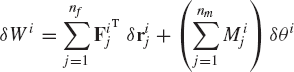
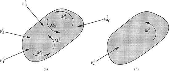
The virtual work of the system of forces shown in Fig. 19b can simply be written as
where rie is the position vector of the point of application of the resultant force Fie.
Since the two systems of forces shown in Fig. 19 are equipollent, one has δWi = δWir, or
If body i is to be in static equilibrium, the following conditions must hold:
which also yield
Substituting these two equations into Eq. 109, one obtains
This is a mathematical statement of the principle of virtual work for the static equilibrium of body i. Equation 112 states that if body i is in static equilibrium, the virtual work of all the forces and moments that act on this body must be equal to zero. This equation can be written as
Equation 113 includes the effect of the external and constraint forces and moments. One may write Eq. 113 as
where δWie is the virtual work of the external forces and moments, and δWic is the virtual work of the constraint forces and moments.
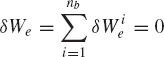
If the mechanical system consists of nb bodies, an equation similar to Eq. 114 can be obtained for each body in the system. By summing up these equations, one obtains
Since joint constraint forces are equal in magnitude and opposite in direction, the virtual work of the constraint forces that act on the system must be equal to zero, that is,
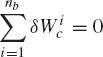
Substituting Eq. 116 into Eq. 115 leads to the principle of virtual work for the static equilibrium of multibody systems as
which implies that the multibody system that consists of interconnected bodies is in static equilibrium if the virtual work of all the external forces acting on the system is equal to zero.
Let a multibody system that consists of nb bodies be subjected to a system of external forces and moments given by
The virtual work of this system of forces and moments is
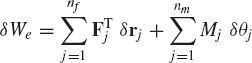
As demonstrated previously, rj and θj can be expressed in terms of the independent coordinates of the system, that is,
where qi is the vector of system independent coordinates or degrees of freedom. Virtual changes in the system coordinates yield
Substituting Eq. 121 into Eq. 119 leads to
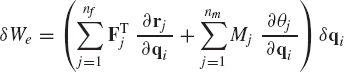
which can be written as
where Qe is the vector of generalized external forces defined as
If the system is in static equilibrium, Eqs. 117 and 123 yield
Since the components of the vector qi are assumed to be independent, one has
This equation implies that if the system is in static equilibrium, the vector of generalized external forces associated with the system degrees of freedom must be equal to zero. Equation 126 represents a system of algebraic equilibrium equations that has a number of equations equal to the number of degrees of freedom of the system. Therefore, these equations can be solved for a number of unknowns equal to the number of degrees of freedom of the system.
It is clear that several basic steps are used in deriving the principle of virtual work for static equilibrium. In the first step, the fact that equipollent systems of forces do the same work is utilized. In the second step, the static equilibrium conditions are used to obtain the principle of virtual work as applied to each body in the system. At this intermediate step, the virtual work of the joint reaction forces must be considered because each body is treated separately. In the third step, the principle of virtual work for the multibody system that consists of a set of interconnected bodies is developed. Since in this step the equilibrium of the entire system is considered, the fact that the virtual work of the joint reaction forces acting on the system is equal to zero is utilized. This step leads to Eq. 117, which is valid regardless of the set of coordinates used. Finally, a set of independent equilibrium conditions is obtained by writing the principle of virtual work in terms of the virtual change in the system degrees of freedom. This step leads to the static equilibrium conditions of Eq. 126.
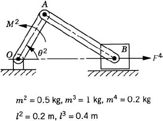
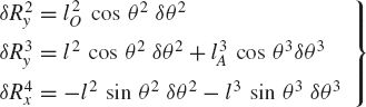
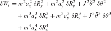
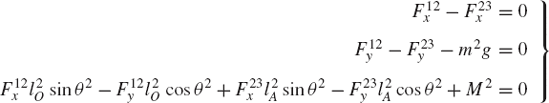
To demonstrate the use of the principle of virtual work in the static equilibrium analysis of multibody systems, the slider crank mechanism shown in Fig. 20 is used. The crankshaft is subjected to an external moment M2, while the slider block is acted upon by a force F4. We assume that the origins of the body coordinate systems are attached to the body centers of mass. To illustrate the process of eliminating the reaction forces, Eq. 113 is first used for the static equilibrium analysis of each body in the mechanism. For the crankshaft, Eq. 113 is given by
where m2 is the mass of the crankshaft, r2O and r2A are, respectively, the global position vectors of points O and A, R2y is the vertical component of the position vector of the center of mass of the crankshaft, and Fij is the vector of the joint reaction forces acting on body j as the result of its connection with body i.
Similarly, the virtual work of the forces acting on the connecting rod can be written as
where m3 is the mass of the connecting rod, r3B is the global position vector of point B, and R3y is the vertical component of the position vector of the center of mass of the connecting rod.
The virtual work of the forces acting on the slider block is also equal to zero. This leads to
Observe that δr2O = 0 since point O is a fixed point, and that δr2A = δr3A and δr3B = δr4B as the result of the conditions of the revolute joints at points A and B, respectively. Also, δR4y = 0, since the slider block moves only in the horizontal direction. Keeping this in mind and adding the preceding three equations leads to Eq. 117 for this mechanism as
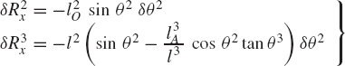
While the reaction forces appear in the static equilibrium equations when the principle of virtual work is applied to each link separately, these reactions are automatically eliminated by adding the resulting equilibrium equations leading to Eq. 130 which contains only the virtual work of the external forces. This equation in its current form is not very useful. In order to make use of this equation we express δR2y, δR3y, δθ2, and δR4x in terms of the system degree of freedom which we may select as θ2. In this case, one has
where l2O is the distance from point O to the center of the crankshaft and l3A is the distance from point A to the center of the connecting rod. Since
one has
Substituting this equation into Eq. 131 yields
Substituting these equations into Eq. 130 leads to
which can be written in the form of Eq. 125 as
where Qe is the generalized force associated with the independent coordinate θ2 and is given by
Since θ2 is an independent coordinate, the scalar Qe of Eq. 136 must be equal to zero, leading to the following algebraic equation:
This equation does not include any reaction forces and can be solved for one unknown. For example, if the external moment M2 is given, one can use the preceding equation to determine the force F4, which is required in order to keep the mechanism in a given static equilibrium configuration.
Example 5.9
The four-bar linkage shown in Fig. 21 is subjected to two external moments M2 and M4 that act, respectively, on the crankshaft and the rocker. If the effect of gravity of the links is neglected and if M2 is assumed to be known, determine the moment M4 that acts on the rocker such that the mechanism is in static equilibrium.
Solution. Since the mechanism is in static equilibrium, the virtual work of all the external forces and moments that act on the mechanism must be equal to zero. This yields
In Example 2, it was shown that
Substituting this equation into the expression for the virtual work, one obtains
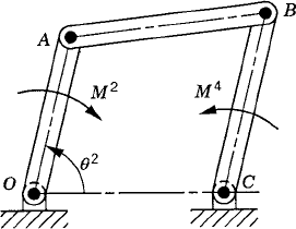
Since the mechanism has one degree of freedom, θ2 can be selected as the independent coordinate. The coefficient of δθ2 in the preceding equation must then be equal to zero, leading to the following equilibrium condition:
from which M4 can be determined as
Example 5.10
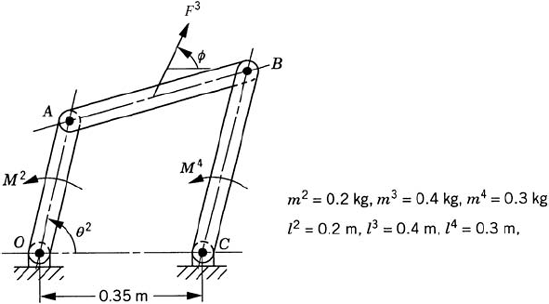
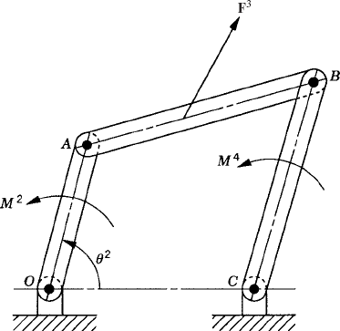
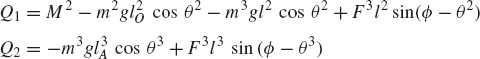
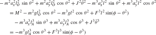
The two-arm robotic manipulator shown in Fig. 22 is subjected to a torque M2 that acts on link 2 and a force F3 that acts at the tip point of link 3, as shown in the figure. The force F3 is assumed to have a known direction defined by the angle ϕ. The mass of link 2 is assumed to be M2, while the mass of link 3 is m3. Considering the effect of gravity, determine M2 and F3 such that the system remains in static equilibrium.
Solution. The virtual work of the forces and moments that act on the system is
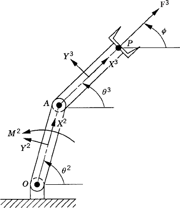
where
These equations yield
Substituting these virtual changes into the expression for the virtual work, and writing F3 in terms of its components F3 cos ϕ and F3 sin ϕ, one obtains
If the system is in static equilibrium, one has δWe = 0, and consequently
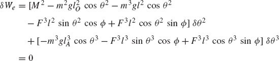
Since θ2 and θ3 are independent coordinates, their coefficients in the preceding equation must be equal to zero. This leads to the following algebraic equations:
The solution of these two equations defines F3 and M2 as
Note that if the gravity of the two links are neglected, M2 and F3 are equal to zero. In this special case, external forces and moments are not required to keep the system in static equilibrium.
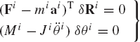
The principle of virtual work can be generalized to study the dynamics of multibody systems that consist of interconnected bodies. In this case, the inertia forces and D'Alembert's principle can be used to establish the principle of virtual work in dynamics. For the rigid body i, the equations of motion are
where Fi is the vector of resultant forces that act on body i, Mi is the sum of the moments about the center of mass, Ai is the acceleration vector of the center of mass,
Using the concept of the equipollent systems of forces discussed in the preceding sections, and without any loss of generality, the force vector Fi can be selected in such a manner that its point of application is the center of mass of the body. One may then multiply the first equation in Eq. 139 by δRi and the second equation by δθi, where Ri is the global position vector of the center of mass of the body. This yields
By adding these two equations, one obtains
or
This equation can be written as
where δWi is the virtual work of the external and reaction forces and moments that act on body i, and δWii is the virtual work of the inertia forces and moments of this body, that is,
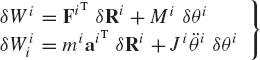
Note that δWi can also be written as
where δWic is the virtual work of the constraint forces and moments, and δWie is the virtual work of the external forces and moments. Substituting Eq. 145 into Eq. 143, one obtains
which implies that when the dynamics of a body is considered separately, the virtual work of the reaction forces acting on the body must be included. It is also important to reiterate at this point that the virtual work of Eq. 146 may be expressed in terms of the actual system of external and reaction forces acting on this body instead of the equipollent system, since both systems produce the same virtual work.
If the mechanical system consists of nb interconnected rigid bodies, the use of Eq. 146 leads to
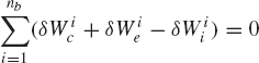
Due to the fact that the joint constraint forces that act on two adjacent bodies are equal in magnitude and opposite in direction, one has
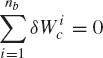
Substituting this equation into Eq. 147 yields
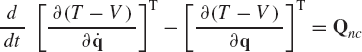
This is the principle of virtual work for dynamics, which states that the virtual work of the external forces and moments acting on the system is equal to the virtual work of the inertia forces and moments of the system. In Eq. 149, one does not need to consider the reaction forces of the workless constraints. Equation 149 can be written as
where
The coefficients of the virtual displacements in Eq. 150 cannot be set equal to zero because these displacements are not independent. To make use of Eq. 150, the virtual changes in the system degrees of freedom are used.
As in the case of the static equilibrium, the virtual displacements can be expressed in terms of the virtual displacements of the independent coordinates. By so doing, the virtual work of the external and inertia forces and moments can be expressed as
where Qe and Qi are, respectively, the vectors of generalized external and inertia forces associated with the system independent coordinates qi. Substituting Eq. 152 into Eq. 150, one obtains
Since the components of the vector qi are assumed to be independent, Eq. 153 leads to
These are the dynamic equations for the multibody system, which imply that the vectors of the generalized external and inertia forces associated with the independent coordinates must be equal. The number of scalar equations in Eq. 154 is equal to the number of degrees of freedom of the system. Consequently, Eq. 154 can be used to solve for a number of unknowns equal to the number of the system degrees of freedom.
The use of the principle of virtual work in dynamics can be demonstrated using the slider crank mechanism discussed in the preceding section and shown in Fig. 20. Since the mechanism has one degree of freedom, the vectors Qe and Qi of Eq. 154 reduce to scalars. It was shown in the preceding section that the generalized external force Qe associated with the angular rotation of the crankshaft is given by

where all the variables in this equation are as defined in the preceding section. The virtual work of the inertia forces is given by
where aix and aiy are the components of the acceleration of the center of mass of link i,
which upon using Eq. 133 yields
Substituting Eqs. 133, 134, and 158 into Eq. 156 yields
which can be written as δWi = Qi δθ2, where
By using Eqs. 154, 155, and 160, the dynamic condition for the slider crank mechanism can be written as
The acceleration components that appear in this equation are not independent by virtue of the kinematic constraints. The relationships between these accelerations can be found by differentiating the algebraic constraint equations, as previously explained. All the acceleration components of the slider crank mechanism can be expressed in terms of θ2,
Example 5.11
Obtain the dynamic equations of the two-arm robotic manipulator of Example 10.
Solution. Since the system has two degrees of freedom, the virtual work of the applied forces can be expressed in terms of the virtual changes in these two degrees of freedom. It was shown in Example 10 that the virtual work of the external forces is
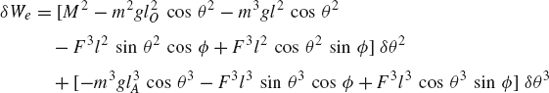
or
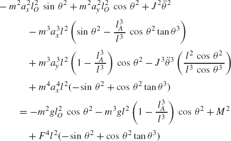
where qi = [θ2 θ3]T, and Qe = [Q1 Q2]T, where
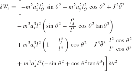
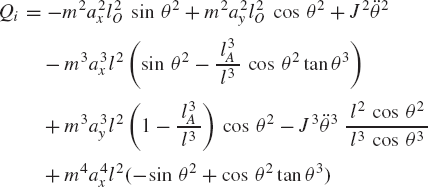
The virtual work of the inertia forces is
where
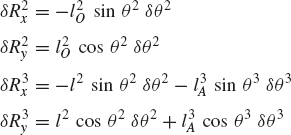
Substituting these virtual changes into the expression of the virtual work of the inertia forces, one obtains
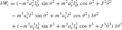
which can be written as
where
in which
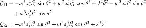
Applying Eq. 154, the dynamic equations for this system are
The principle of virtual work allows us to formulate the dynamic equations using any set of independent generalized coordinates. Lagrange (1736–1813) created this powerful tool, recognized its superiority in formulating the dynamic equations, and used it as the starting point to formulate Lagrange's equation, which we will discuss in this section.
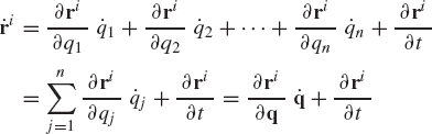
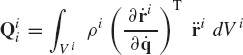
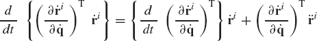
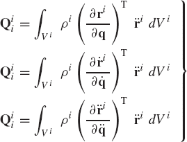
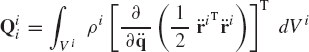
The virtual work of the inertia forces of a rigid body i is defined as
where ρi and Vi are, respectively, the mass density and volume of the rigid body, and ri is the global position vector of an arbitrary point on the rigid body. The global position vector of the arbitrary point can be written in terms of the system generalized coordinates as
It follows that
Substituting Eq. 164 into Eq. 162, the virtual work of the inertia forces of the rigid body i can be written as
or
where

is the vector of generalized inertia forces of body i associated with the system generalized coordinates q.
We note also that the absolute velocity vector of the arbitrary point on the rigid body is
from which one can deduce the following identity:

By using a similar procedure, one can also show that
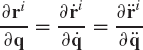
By using the identity of Eq. 169, the generalized inertia forces of the rigid body i given by Eq. 167 can be written as
Note that
which upon utilizing the identity of Eq. 169 leads to
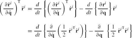
Substituting Eq. 173 into Eq. 171 and using the definition of the kinetic energy of body i
the generalized inertia forces of the rigid body i can be expressed in terms of the body kinetic energy as
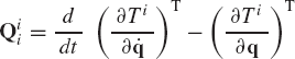
The inertia forces of a system of nb rigid bodies can then be written as
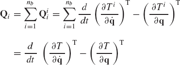
where T is the system kinetic energy defined as
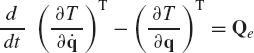
Using the principle of virtual work in dynamics, one concludes that if the generalized coordinates are independent, the system equations of motions can be written as
where qj, j = 1, 2, ..., n are the independent coordinates or the system degrees of freedom and Qj is the generalized applied force associated with the independent coordinate qj. Equation 177 is called Lagrange's equation of motion.
Example 5.12
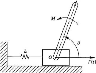
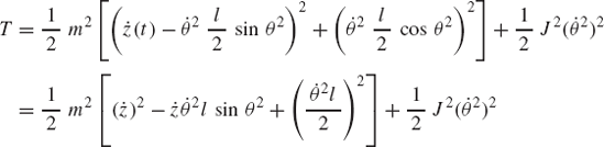
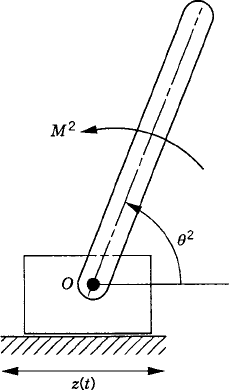
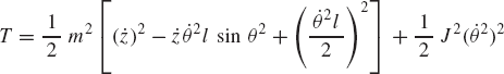
To demonstrate the use of Lagrange's equation, we consider the system shown in Fig. 23. The rod in this system is assumed to be uniform and has mass m2, mass moment of inertia about its center of mass J2, and length l. The block is assumed to have a specified motion z(t) and, consequently, the system has one degree of freedom, which we select to be the angular orientation of the rod θ2. The kinetic energy of the rod can be written as
where R2x and R2y are the Cartesian components of the position vector of the center of mass of the rod. These coordinates are defined as
and their time derivatives are
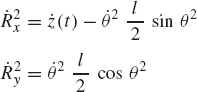
The kinetic energy of the rod takes the form
The virtual work of the external forces acting on the rod is
where Qe is the generalized force associated with the system degree of freedom θ2 and is defined as
Lagrange's equation of motion of this system can then be written as
where
It follows that
in which
One also has
Substituting the preceding equation into Eq. 177, one obtains
Clearly, this equation can also be derived using D'Alembert's principle by equating the moments of the applied and inertia forces about point O. The use of D'Alembert's principle to obtain the above equation was demonstrated in the preceding chapter. A third alternative for deriving this equation is to use the principle of virtual work, which is the starting point in deriving Lagrange's equation.
The identity of Eq. 170 clearly demonstrates that the virtual work of the inertia forces of the rigid body i can be evaluated using any of the following expressions:
or by using the expression of the kinetic energy in Lagrange's equation as previously discussed. All of these forms are equivalent and lead to the same results when the same set of coordinates are used.
While in Lagrange's equation, the generalized inertia forces are expressed in terms of the kinetic energy which is quadratic in the velocities; in Gibbs-Appel equation, the generalized inertia forces are expressed in terms of an acceleration function. The Gibbs-Appel form of the inertia forces can be obtained using the third equation in Eq. 178. This equation can be written as
which can also be written as

where Si is an acceleration function defined as
The forces acting on a mechanical system can be classified as conservative and nonconservative forces. If Qe is the vector of generalized forces acting on the multibody system, this vector can be written as
where Qco and Qnc are, respectively, the vectors of conservative and nonconservative forces. As pointed out previously, conservative forces can be derived from a potential function V, that is,
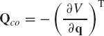
where q = [q1 q2 ... qn]T is the vector of generalized coordinates of the multibody system. Substituting Eq. 183 into Eq. 182, one obtains
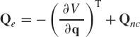
If the generalized coordinates are independent, Lagrange's equation can be written in the following form:
Using Eqs. 184 and 185 and keeping in mind that the potential function V does not depend on the generalized velocities, one gets
In terms of the Lagrangian, Lagrange's equation takes the form
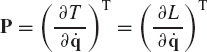
If the multibody system has n degrees of freedom, Lagrange's equation defines n second-order differential equations of motion expressed in terms of the degrees of freedom and their time derivatives. The Hamiltonian formulation, on the other hand, leads to a set of first-order differential equations defined in terms of the generalized coordinates and generalized momenta Pi, which are defined as
In obtaining Eq. 189, the fact that the potential energy is independent of the velocities is utilized. This equation can be used to define the vector of generalize momenta as
The Hamiltonian H is defined as
and
It is clear from the definition of the vector of the generalized momenta of Eq. 190 that the second and third terms on the right side of the preceding equation cancel. Consequently,
Using Eq. 190, the generalized velocity vector can be expressed in terms of the generalized momenta. If the results are substituted into Eq. 191, the Hamiltonian can be expressed in terms of the generalized coordinates and momenta as
If follows that
Comparing Eqs. 193 and 195, it is clear that
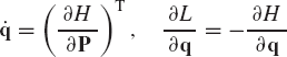
Using these identities and Eq. 188, one obtains the following set of 2n first-order differential equations:
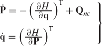
These equations are called the canonical equations of Hamilton. The 2n first-order differential equations replace the n second-order differential equations that can be derived using the principle of virtual work or Lagrange's equation. In order to use the canonical equations, one first needs to define the Lagrangian L as a function of the coordinates and velocities using Eq. 187. The vector of generalized momenta can then be defined using Eq. 190. The generalized momenta and the Lagrangian can be used to define the Hamiltonian H using Eq. 191. The first-order differential equations of the system can be obtained by substituting the Hamiltonian H into Eq. 197.
In principle, the principle of virtual work, Lagrange's equation, Gibbs-Appel equation, and the canonical equations of Hamilton can be used to define the same set of differential equations. The answer to the question of which method is better for formulating the dynamic equations depends on the application. In computational dynamics wherein the interest is focused on developing general solution procedures, it is not clear what advantage each method can provide as a computational tool since all these methods can be used to obtain the same equations.
Example 5.13
It was shown in Example 12 that the kinetic energy of the system shown in Fig. 23 is given by
The potential energy of the system is
The Lagrangian L is then given by
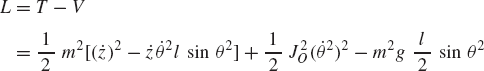
where J2O is the mass moment of inertia of the rod about point O. Since the system has one degree of freedom, the generalized momentum is defined as
The preceding equation can be used to express
The Hamiltonian is defined as

Substituting for
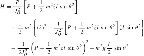
The first-order equations of the system can then be obtained using Eq. 197 as
A generalized coordinate that does not appear in the Lagrangian l is called cyclic or ignorable. Cyclic or ignorable coordinates are also absent from the Hamiltonian H. For a cyclic coordinate qk, one has
If there are no nonconservative forces associated with the cyclic coordinate qk, Eq. 197 yields
The total time derivative of the Lagrangian L is given by
Substituting Eq. 199 into the preceding equation, one gets
which yields
or equivalently,
Since the potential energy function is independent of the velocities, one has
Using this equation, Eq. 203 can be written as
which implies that
That is, in the case of a conservative system, the Hamiltonian H is a constant of motion. We also note that since
the Hamiltonian H takes the following form:
which implies that, for a conservative system, the Hamiltonian is the sum of the kinetic and potential energies of the system and it remains constant throughout the system motion.
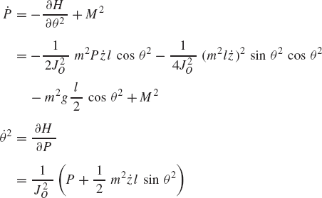
Example 5.14
Figure 24 shows a homogeneous circular cylinder of radius r, mass m, and mass moment of inertia J about its center of mass, where J = m(r)2/2. The cylinder rolls without slipping on a curved surface of radius R. Use the principle of conservation of energy to derive the equation of motion of the cylinder.
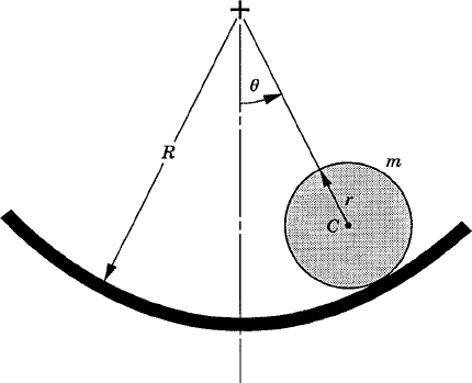
Solution. The kinetic and potential energies of the cylinder are
where vc is the absolute velocity of the center of mass of the cylinder and ω is its angular velocity, both defined as
Substituting from these two equations into the expression of the kinetic energy, we obtain
The Hamiltonian H is
Since the Hamiltonian is constant,
which yields the equation of motion of the cylinder
The results obtained previously in this chapter for the slider crank mechanism shown in Fig. 20 using the principle of virtual work can also be obtained using the Gaussian elimination and the equations of the static equilibrium. Figure 25 shows the forces acting on the links of the slider crank mechanism. The equations of the static equilibrium of the crankshaft can be written as
The equations of the static equilibrium of the connecting rod are
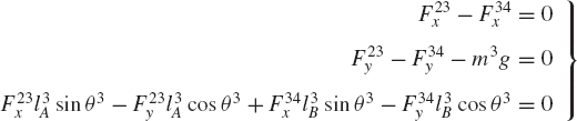
The equation of the static equilibrium fo the slider block is
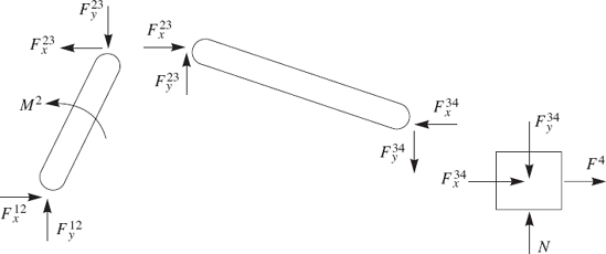
The preceding seven equations of the static equilibrium of the three links of the slider crank mechanism can be rearranged and written in the following matrix form:
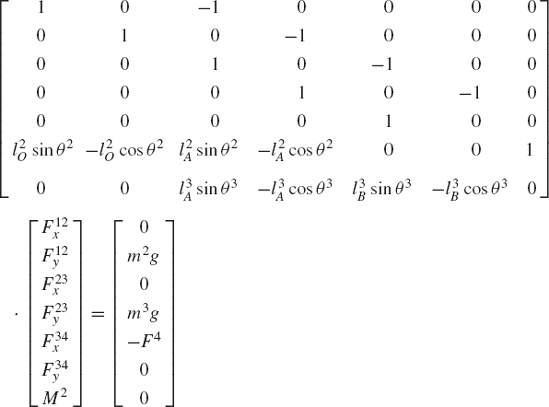
In this matrix equation it is assumed that the unknowns are the external moment M2 and the components of the reaction forces F12x, F12y, F23x, F23y, F34x, and F34y. A standard Gaussian elimination procedure can be used to obtain an upper triangular form of the coefficient matrix in the preceding equation. This Gaussian elimination procedure leads to
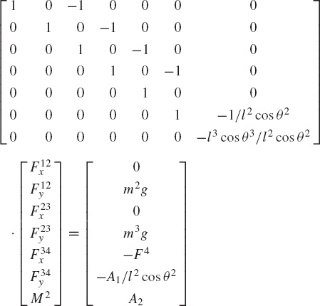
where
Equation 123 can be solved for M2 as
which is the same equation obtained earlier in this chapter (Section 6) using the principle of virtual work.
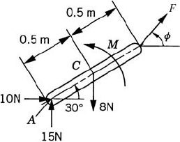
For the rod shown in Fig. P1, assume that F = 5 N, M = 3 N · m, and ϕ = 45°. Assuming that the generalized coordinates of the rod are the Cartesian coordinates of point A and the angular orientation of the rod, determine the generalized forces associated with these generalized coordinates.
Repeat problem 1 assuming that the generalized coordinates of the rod are the Cartesian coordinates of point C and the angular orientation of the rod.
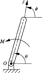
For the system shown in Fig. P2, let θ be the independent generalized coordinate of the rod. Determine the generalized forces associated with this generalized coordinate. Neglect the effect of gravity.
Repeat problem 3 taking into consideration the effect of gravity.
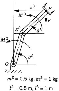
For the system shown in Fig. P3, let F=10 N, M2 = 3 N · m, M3 = 3 N · m, θ2 = 45°, and θ3 = 30°. Determine the generalized forces associated with the generalized coordinates θ2 and θ3. Neglect the effect of gravity.
Repeat problem 5 taking into account the effect of gravity.
Repeat problem 5 assuming that the generalized coordinates are x2 and x3.
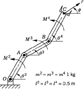
For the system shown in Fig. P4, write the virtual changes in the position vector of point C in terms of the virtual change in the independent generalized coordinates θ2, θ3, and θ4.
For the system shown in Fig. P4, obtain the generalized forces associated with the generalized coordinates θ2, θ3, and θ4. Assume θ2 = 45°, θ3 = 30°, θ4 = 45°, ϕ = 30°, F = 10 N, M2 = 10 N · m, M3 = 8 N · m, and M4 = 3 N · m. Consider the effect of gravity.
For the slider crank mechanism shown in Fig. P5, assume that θ2 = 45°, M2 = 10 N · m, and F4 = 10 N. Determine the generalized force associated with the independent generalized coordinate θ2. Consider the effect of gravity.
Repeat problem 10 assuming that the independent generalized coordinate is the location of the slider block.
For the four-bar linkage shown in Fig. P6, obtain the generalized force associated with the independent generalized coordinate θ2. Assume that θ2=60°, ϕ=30°, M2=5 N · m, F3 = 3 N, and M4 = 5 N · m. Consider the effect of gravity.
Repeat problem 12 assuming that the generalized coordinate is selected to be the angular orientation of the coupler θ3.
Repeat problem 12 assuming that the generalized coordinate is selected to be the angular orientation of the rocker θ4.
For the unconstrained rod shown in Fig. P1, determine F, m, and ϕ such that the rod is in static equilibrium. Use the principle of virtual work.
For the system shown in Fig. P2, let θ = 45°, F = 5 N, and ϕ = 60°. Assume that the mass and length of the rod are 1 kg and 1 m, respectively. Determine the moment m such that the system is in static equilibrium position. Use the principle of virtual work and consider the effect of gravity.
For the system shown in Fig. P2, let the length of the rod be 1 m, θ = 45°, F = 5 N, M = 3 N · m, and ϕ = 60°. Using the principle of virtual work determine the weight of the rod such that the system is in static equilibrium position.
Use the principle of virtual work in statics to determine the joint torque M2 and m3 of the system shown in Fig. P3. Assume that θ2 = 45°, θ3 = 30°, and F = 5 N. Consider the effect of gravity.
For the system shown in Fig. P3, let M2 = 3 N · m, M3 = 5 N · m, F = 5 N. Does a static equilibrium configuration exist for this system? Use the principle of virtual work to find the answer and consider the effect of gravity.
For the system shown in Fig. P4, let θ2 = 45°, θ3 = 30°, θ4 = 45°, ϕ = 30°, and F = 5 N. Use the principle of virtual work to determine M2, M3, and M4 such that the system is in static equilibrium. Consider the effect of gravity.
Use the principle of virtual work in statics to determine the input torque M2 of the slider crank mechanism shown Fig. P5. Assume that θ2 = 45° and F4 = 4 N. Take into consideration the effect of the gravity. Assume that the generalized coordinate is the joint angle θ2.
Repeat problem 21 assuming that the generalized coordinate is the horizontal position of the slider block.
Use the principle of virtual work in statics to determine the input torque M2 of the four-bar linkage shown in Fig. P6. Consider the generalized coordinate to be the crank angle θ2. Consider the effect of gravity and assume that θ2 = 60°, ϕ = 45°, F3 = 5 N, and M4 = 5 N · m.
Repeat problem 23 assuming that the generalized coordinate is the orientation of the coupler θ3.
Repeat problem 23 assuming that the generalized coordinate is the orientation of the rocker θ4.
Use the principle of virtual work in statics to determine the output torque M4 that acts on the rocker of the four-bar linkage shown in Fig. P6. Assume that θ2 = 60°, ϕ = 45°, F3 = 5 N, and M2 = 5 N · m. Consider the crank angle θ2 as the generalized coordinate. Take the effect of gravity into consideration.
Repeat problem 26 assuming that the generalized coordinate is the rocker angle θ4.
The components of the acceleration of the center of mass of the rod shown in Fig. P1 are ax = 50m/s2, ay = 120m/s2. The angular acceleration of the rod is assumed to be 500 rad/s2. The rod is assumed to be slender and uniform with mass 1 kg. Use the principle of virtual work in dynamics to determine m, F, and ϕ. Consider the effect of gravity.
For the system shown in Fig. P2, let θ = 45°, ϕ = 60°, F = 10 N. The rod shown in the figure is assumed to be uniform and slender with mass 1 kg and length 1 m. The angular velocity and angular acceleration of the rod are assumed to be

Repeat problem 29 assuming that the angular acceleration

Use the principle of virtual work in dynamics to determine the joint torques M2 and m3 for the system shown in Fig. 5-28. Use the following data: θ2 = 45°, θ3 = 30°,

The system shown in Fig. P4 consists of three uniform slender rods that are connected by revolute joints. Let θ2 = 45°, θ3 = 30°, θ4 = 45°,
Determine the joint reaction forces in problem 31.
Determine the joint reaction forces in problem 32.
The crankshaft and connecting rod of the slider crank mechanism shown in Fig. P5 are assumed to be uniform slender rods. Use the principle of virtual work in dynamics to determine the input torque M2. Use the following data: θ2 = 45°,
Repeat problem 35 assuming that

Determine the joint reaction forces in problem 35.
Determine the joint reaction forces in problem 36.
The crankshaft, coupler, and rocker of the four-bar linkage shown in Fig. P6 are assumed to be uniform slender rods. Assume that θ2 = 60°,
Repeat problem 39, assuming the rocker angle θ3 as the generalized coordinate.
Repeat problem 39, assuming the coupler angle θ4 as the generalized coordinate.
Determine the joint reaction forces in problem 39.
Repeat problem 39 assuming that
The system shown in Fig. P7 consists of a slider block of mass m2 and a uniform slender rod of mass m3, length l3, and mass moment of inertia about its center of mass J3. The slider block is connected to the ground by a spring that has a stiffness coefficient k. The slider block is subjected to the force F(t), while the rod is subjected to the moment m. Obtain the differential equations of motion of this two-degree-of-freedom system using Lagrange's equation.
Determine the generalized inertia forces of the system of problem 44 using the three different equations given in Eq. 178. Compare the results obtained using these three equations with the results obtained using Lagrange's equation.
Derive the differential equations of motion of the system of problem 44 using the Gibbs—Appel equation.