
4
Economics and Corrosion
Mahsa Mostashar-Nezami∗
CEO and Founder of ATAVART, Privately Held co., Tehran, Iran
4.1 Introduction
I try to consider corrosion as a factor which impacts an economy because it contains a vast amount of product. The NACE report in 2013 said 3.4% of the world's products deplete in the corrosion processes [1], and a considerable percentage of this cost is avoidable.
In this chapter, first, you will be familiarized with some of the main principles of Economics. Economics is the knowledge of big pictures. To show the essential trace of every engineer's work in an economy, it is important that they can imagine how their work and their occupation impacts the economy. To address this idea in this chapter, there are two main sections: Economics and Corrosion Economics.
In the first section, I try to teach the basic economic principles and show this complex view, and then bring some of the most useful economics approaches to estimating a productive society.
In the second section, two methods for estimating corrosion cost must be considered. The first one, the I/O, is a time‐consuming and difficult method for estimating corrosion costs. The results of the I/O method are accurate and reliable but I suggest this method use in nation‐wide or heterogeneous projects. The second method is about the life cycle cost (LCC) method and there are many different ways to calculate cost with this method. It is easier to to measure than the I/O method and is suggested to use with small or medium sized projects.
In the last section, try to show the impact of corrosion on sustainability, as it is important to show the readers how their job affects lives for many years; this allows them keep a closer watch on their actions. I choose sustainability rather than socio‐economic or environmental impact because sustainability contains both the social and environmental impact of corrosion, and also takes economics into account.
In this chapter, the words shown in italic emphasize the importance of understanding the meaning of the content.
4.2 Economics
This section aims to familiarize engineers with some basic economics definitions such as gross domestic product (GDP), what it is, and its different measurement methods; and present value (PV), and so on.
In this section, I try to be as brief with these principles as I can; for this reason, reading the charts and tables carefully is important for understanding the content.
4.2.1 What Is Economics
Economics is the knowledge of coping with scarcity. It means that economics follow our unlimited needs within limited resources. There are some conflicts to classify economics as a science or art. In the Avestan and Pahlavi languages, which were the ancestors of the today's Persian Language and the decedent of the Indo‐European languages, the word art can be used with two parts “hu” and “nara.” The part “hu” means good, well, beautiful, very, sufficient, expressive, strong, and steadfast; and “nara” refers to the human [2]. With this means is economics is an art because it tries to structure human behavior in a sensible and sufficient way.
Economics is almost a young major in contrast with, for instance, Mathematics or chemistry. In the past 250 years, philosophers had tended to this knowledge. Gradually, this major will segregate from philosophy. Macroeconomics appears as a separate subject within economics in the 1930s, when the great depression occurred [3]. Today, we have many economics subjects such as macroeconomics, microeconomics, international economics, and economic development. There are also some interdisciplinary subjects such as environmental economics, socio‐economics, and so on. In recent years, an important major has emerged; sustainable development, which considers the unity between economics, the environment, and aspects of society. In this section, I will speak about macroeconomics first, then and try to explain the corrosion impact on sustainability in the last section.
The above mentioned subjects are about mainstream economics, but we have two kinds of economists; the Heterodox Economists and Orthodox Economists. The heterodox economists are those who do not accept the basic underlying models used by a majority of economists as the most useful model for analyzing the economy [3], while the orthodox economists accept the mainstream principles of economics.
There are six heterodox approaches; Austrian, Post‐Keynesian, Institutionalist, Radical, Feminist, and Religious.1 One of most the famous approaches in the Radical view is Marxian economics. Radical economists are much more prepared to discuss social conflict and stresses in our society than are mainstream economics. The characteristic of many heterodox economists is their analysis tends to be less formal than the mainstream. The less formal is not about whether right or wrong, or better or worse, because in the actual situation it is difficult to say precisely what the logic is [3]. On another side of less informal economists are mainstream economists trying to explain people's behavior with many strict models.
Macroeconomics focuses on the big picture of a society or the whole of the world. The specific focus of macroeconomics are the big four issues. These four issues are inflation, unemployment, the rate of Economic growth, and business cycles (fluctuations in the economy) [4].
Two main economic theories are Classical and Keynesian. The most challenging issue between these two theories is the size of government and its interference. In 1776 when Adam Smith wrote his well‐known book “The Wealth of Nations” the world population had half a million people [5]. It is understandable with this population that Adam Smith believed in an endogenous adjusted system he introduced as his famous idea, “invisible hand.” Thus, he believed in the minimum government interference, and a system that corrects itself automatically in the long run and provides full employment. In the 1930s during the great depression, Professor John Maynard Keynes challenged this condition in the neoclassical idea and said his famous quote, “In the long run we are all dead.” He brings the short and medium term correction by the interference of the government. Although his idea was challenged in the 1970s by these years' stagflation, his recommendations could not solve this problem, and the Monterey economics birthed. However, today's governmental policies are almost a mix of these views.
Today's mainstream economics are based on Alfred Marshal’s theory on supply and demand, and he is the founder of neoclassical economics. In addition, he brings the ideas of supply and demand in the book “Principles of Economics” in 1890 [6]. His theory is the fundamental theory of today's economics; the supply and demand are about the aggregate supply and demand of the goods and services in an economy.
There are vast principles in economics, but in this chapter, I prefer to introduce the most useful principles will need to understand in the model of corrosion estimation.
4.2.2 Gross Domestic Product
Understanding the operation of the real world is the aim of macroeconomics [7]. To measure an economy, we focus on what happens in the entire economy and its relationship with other countries. In an economy, we have two main parts which allocate its resources; the government and the private sector. The private sector is divided into two parts: households and firms. Thus, households, firms, the government, and the rest of the world are the four main parts of an economy.
We need some definitions to understand how economists try to measure the GDPs of an economy.
First, they know two kinds of users for goods and services; final users and intermediate users. Second, they separate the goods and services produced in the entire economy in three ways; final goods, intermediate goods, and value‐added goods.
Final users are the ones who buy goods and services for their daily life consumption. Households purchasing furniture for their home, or an administration purchasing a laser printer for their daily work are final users. However, the intermediate users are the one buy the goods for their production; for instance, a furniture manufacturer buys leather for their goods.
Final goods and services are the final users who buy and use these goods in their daily life. For example, we buy dairy goods for our meals; these dairy goods are the final goods. Intermediate goods are from the manufacturers that buy or produce their goods and sell them to other intermediate users or final users. For example, packets a dairy manufacture purchases for their goods are the intermediate goods. Some of the products are intermediate goods sold to other intermediate users; for example, some petrochemical products are examples of these intermediate goods.
Familiarizing ourselves with these kinds of users, goods, and services is essential; because when measuring the GDP we use the final goods for final users.
GDP calculation: Three different methods of estimating the GDP are (i) Expenditure, (ii) Income, and (iii) Product or value‐added approaches.
The expenditure approach added all of the final goods and service values for an economy within a given time.
The income approach added all of the income – wages, rents, interest, and profits – that all production factors earn to produce final goods and services in a given time [8].
The product or value‐added approach adds the value of primary goods with the value of the products to produce the final goods. For example, if a firm purchased wood, leather, glue, and screws for their production with a sum up to $100, and sold their products to the final customer for $250, this method added $100 for primary goods and $150 for a value that add to these materials, which may contain some other intermediate materials and services.
These three types of estimation have an equal value to each other. In the following tables which introduce these three measurements of GDP, compare the amount of GDP to each other.
4.2.2.1 The Expenditure Approach
The most useful method which economists use for measuring the GDP is the expenditure approach. The GDP is equal to the total expenditures for all final goods and services produced within the country in a stipulated period [9].
Y is GDP; C is personal consumption expenditure (PCE); I is Investment, gross private domestic investment; G is Government consumption expenditure and gross investment; NX is Net export, Export minus Import. Table 4.1 shows this method for USA GDP in 2019.
Personal Consumption expenditures (C) consist of expenditure people pay for goods and services. Goods includes durable goods and nondurable goods. Durable goods are something that lasts for a long time (usually for more than one year); motor vehicles and parts, furnishings and durable household equipment, and recreational. Nondurable goods are those that last for less than one year; basically a citizen's daily life consumptions. Food and beverages purchased for off‐premise consumption, clothing and footwear, gasoline or other energy goods, and other items. Services consist of household consumption expenditures (for services) and final consumption expenditures of nonprofit institutions serving households. Household consumption expenditures contain housing and utilities, health care, transportation services, recreation services, food services, insurance, and other services. Final consumption expenditures of nonprofit institutions serving households contain the gross output of nonprofit institutions minus receipts from sales of goods and services by nonprofit institutions.
PCEs are the highest part of the GDP for 2019; reaching 67.9% of the GDP of the United States.
Gross private investment (I) consists of fixed investment and change in private inventories. Fixed investment has two parts; nonresidential and residential investment. Nonresidential investment contains structures, equipment, and intellectual property products. Change in private inventories includes farm and nonfarm investment. Gross private investment contains 17.5% of the GDP. Almost all of these investments are about fixed and nonresidential investments.
Net exports and imports (NX) include exports and imports of goods and services. A trade deficit occurs when the number of goods and services a country imports is more than goods and services export. The United States mostly has a trade deficit, and it was −2.8% of GDP in 2019.
Government consumption expenditures and gross investment (G) have two parts; federal, and state and local for the US. Federal consists of national defense and nondefense, and state and local consists of government consumption expenditures and gross investment. The government consumption expenditure and gross investment was 17.5% of the GDP in 2019, and most of it was from consumption expenditures of states and local governments.
Table 4.1 GDP, expenditure approach (billions of dollars).
Source: U.S. Bureau of Economic Analysis. [Online]; 2020 [cited 10 19 2020. Available from: https://apps.bea.gov/scb/2020/08‐august/0820‐nipa‐update.htm#pce.
| Line | 2019 | Share of GDP | |
|---|---|---|---|
| 1 | Gross domestic product (GDP) | 21 747.4 | 100.0 |
| 2 | Personal consumption expenditures | 14 759.2 | 67.9 |
| 3 | Goods | 4562.4 | 21.0 |
| 4 | Durable goods | 1554.1 | 7.1 |
| 9 | Nondurable goods | 3008.2 | 13.8 |
| 14 | Services | 10 196.8 | 46.9 |
| 26 | Gross private domestic investment | 3732.6 | 17.2 |
| 27 | Fixed investment | 3729.2 | 17.1 |
| 28 | Nonresidential | 2902.3 | 13.3 |
| 29 | Structures | 652.3 | 3.0 |
| 30 | Equipment | 1229.3 | 5.7 |
| 35 | Intellectual property products | 1020.7 | 4.7 |
| 39 | Residential | 827.0 | 3.8 |
| 40 | Change in private inventories | 3.4 | 0.0 |
| 43 | Net exports of goods and services | −549.8 | −2.5 |
| 44 | Exports | 2515.7 | 11.6 |
| 45 | Goods | 1629.1 | 7.5 |
| 46 | Services | 886.5 | 4.1 |
| 47 | Imports | 3065.4 | 14.1 |
| 48 | Goods | 2460.7 | 11.3 |
| 49 | Services | 604.8 | 2.8 |
| 50 | Government consumption expenditures and gross investment | 3805.3 | 17.5 |
| 51 | Federal | 1447.9 | 6.7 |
| 52 | National defense | 874.7 | 4.0 |
| 55 | Nondefense | 573.3 | 2.6 |
| 58 | State and local | 2357.4 | 10.8 |
4.2.2.2 The Income Approach
Another approach for measuring the nation's economy is the income approach. This approach counts the income earned and costs spent during production. The Gross domestic income (GDI) should equal the GDP because of the different sources used to measure it. You can see this method in Table 4.2 for USA income in 2019. There are some differences between these two kinds of measurements and is known as the “statistical discrepancy.”2
The name of the accounts in this table can show which activity counts; but an account that is less speaks about is the consumption of fixed capital (CFC).
CFC is an account considered to degrade and corrode the economy’s capital. This item was $3474.4 billion in 2019, and most of this includes the private sector. In the Bureau of Economic Analysis, this account is defined as, “The charge for the using up of private and government fixed capital located in the United States. It is the decline in the value of the stock of fixed assets due to wear and tear, obsolescence, accidental damage, and aging. For general government and for nonprofit institutions that primarily serve individuals, CFC serves as a measure of the value of the current services of the fixed assets owned and used by these entities” [10]. The System of National Accounts (SNA) defined this as, “Consumption of fixed capital (CFC); the decline in the value, in current prices, of the stock of capital goods held by producers resulting from physical deterioration, normal obsolescence, or normal accidental damage” [11].
In the later sections we speak about this account in more depth.
4.2.2.3 The Value‐Added Approach
The value‐added approach is another source for measuring economic production. It concerns the values that each institutional unit adds to the components which produces a good or service. This approach estimates the sum of employee compensation, taxes on production, and imports fewer subsidies and gross operating surplus. Table 4.3 explains this approach. Each item in the following table includes one of these three components. In the following table, you can see the share of industries in domestic production.
As you can see, these three types of measuring the GDP are almost equal, but the points of view are different.
4.2.2.4 Income, Consumption, Saving, and Investment
Saving and investment are two factors related to the main topic of this section. To explore these two factors, we must familiarize ourselves with the relation between income, investment, consumption, and saving. All of the consumption, investment, or saving in the private and governmental sectors include these items.
In an economy, income is distributed between savings or consumption. Thus, this relation is between these three items:
where Y is the income of the economy, C is consumption, and S is savings. Savings is the part of income that society prefers to put away without spending, for example, in a bank account.
On the other side, this relation is between consumption and income:
C0 is the undebatable consumption in an economy and is called autonomous expenditure.
There is another definition for C and Y:
Where MPC means marginal propensity consumption.
Furthermore, this relation is between saving and income.
Also, marginal saving is:
The relation below is between marginal consumption and marginal savings:
In sum,
This equation shows the relation between savings and consumption in an economy. As you can see, if autonomous consumption increased, the level of savings would decrease.
4.2.2.4.1 Investment
Investment is an expenditure society spends on capital stock, such as renewing factory machinery, infrastructure repair and maintenance, or construction of a building. In economics, saving and investment must be equal, which means all of the income savings must be spent for investment in an economy; however, in the real world, these are not the same. Most of the world's countries' investments are more than their savings because they have foreign investments. In the expenditure approach, this item was 17.2% of US GDP in 2019.
From corrosion points of view, while the amount of money spent on corrosion issues such as repairing and maintenance belong to the consumption items, the amount of money spent on investment to capital stocks decreases. Spending money on investment helps society in growth and development. In Table 4.2 this amount shows in the CFC account.
Table 4.2 Gross domestic income by type of income (billions of dollars).
Source: U.S. Bureau of Economic Analysis, September 30, 2020 – Next Release Date October 29, 2020.
| Gross domestic income (GDI) | 21 721.2 |
| Compensation of employees, paid | 11 577.4 |
| Wages and salaries | 9435.1 |
| To persons | 9415.7 |
| To the rest of the world | 19.4 |
| Supplements to wages and salaries | 2142.4 |
| Taxes on production and imports | 1509.6 |
| Less: Subsidies 1 | 81.1 |
| Net operating surplus | 5240.8 |
| Private enterprises | 5248.7 |
| Net interest and miscellaneous payments, domestic industries | 808.9 |
| Business current transfer payments (net) | 152.0 |
| Proprietors' income with inventory valuation and capital consumption adjustments | 1697.7 |
| Rental income of persons with capital consumption adjustment | 795.5 |
| Corporate profits with inventory valuation and capital consumption adjustments, domestic industries | 1794.6 |
| Taxes on corporate income | 312.3 |
| Profits after tax with inventory valuation and capital consumption adjustments | 1482.3 |
| Net dividends | 968.7 |
| Undistributed corporate profits with inventory valuation and capital consumption adjustments | 513.6 |
| Current surplus of government enterprises1 | −7.9 |
| Consumption of fixed capital | 3474.4 |
| Private | 2878.9 |
| Government | 595.6 |
| Addendum: | |
| Statistical discrepancy | 26.2 |
Table 4.3 Value added by industry (billions of dollars).
Source: U.S. Bureau of Economic Analysis, Last Revised on: September 30, 2020.
| Line | 2019 | |
|---|---|---|
| 1 | Gross domestic product | 21 747.4 |
| 2 | Private industries | 19 075.1 |
| 3 | Agriculture, forestry, fishing, and hunting | 180.4 |
| 4 | Farms | 140.1 |
| 5 | Forestry, fishing, and related activities | 40.3 |
| 6 | Mining | 300.6 |
| 7 | Oil and gas extraction | 188.8 |
| 8 | Mining, except oil and gas | 60.9 |
| 9 | Support activities for mining | 50.8 |
| 10 | Utilities | 340.6 |
| 11 | Construction | 905.5 |
| 12 | Manufacturing | 2370.1 |
| 13 | Durable goods | 1328.0 |
| 14 | Wood products | 42.1 |
| 15 | Nonmetallic mineral products | 65.9 |
| 16 | Primary metals | 63.1 |
| 17 | Fabricated metal products | 161.7 |
| 18 | Machinery | 162.5 |
| 19 | Computer and electronic products | 308.3 |
| 20 | Electrical equipment, appliances, and components | 66.2 |
| 21 | Motor vehicles, bodies and trailers, and parts | 164.7 |
| 22 | Other transportation equipment | 164.3 |
| 23 | Furniture and related products | 31.4 |
| 24 | Miscellaneous manufacturing | 97.7 |
| 25 | Nondurable goods | 1042.1 |
| 26 | Food and beverage and tobacco products | 270.1 |
| 27 | Textile mills and textile product mills | 17.0 |
| 28 | Apparel and leather and allied products | 9.2 |
| 29 | Paper products | 61.2 |
| 30 | Printing and related support activities | 40.5 |
| 31 | Petroleum and coal products | 161.7 |
| 32 | Chemical products | 398.0 |
| 33 | Plastics and rubber products | 84.4 |
| 34 | Wholesale trade | 1270.4 |
| 35 | Retail trade | 1180.3 |
| 36 | Motor vehicle and parts dealers | 228.5 |
| 37 | Food and beverage stores | 163.0 |
| 38 | General merchandise stores | 154.1 |
| 39 | Other retail | 634.7 |
| 40 | Transportation and warehousing | 710.0 |
| 41 | Air transportation | 150.0 |
| 42 | Rail transportation | 43.6 |
| 43 | Water transportation | 15.0 |
| 44 | Truck transportation | 176.8 |
| 45 | Transit and ground passenger transportation | 57.1 |
| 46 | Pipeline transportation | 51.8 |
| 47 | Other transportation and support activities | 136.7 |
| 48 | Warehousing and storage | 79.0 |
| 49 | Information | 1156.1 |
| 50 | Publishing industries, except internet (includes software) | 313.3 |
| 51 | Motion picture and sound recording industries | 90.0 |
| 52 | Broadcasting and telecommunications | 471.9 |
| 53 | Data processing, internet publishing, and other information services | 280.9 |
| 54 | Finance, insurance, real estate, rental, and leasing | 4615.5 |
| 55 | Finance and insurance | 1693.2 |
| 56 | Federal Reserve banks, credit intermediation, and related activities | 721.5 |
| 57 | Securities, commodity contracts, and investments | 309.2 |
| 58 | Insurance carriers and related activities | 632.4 |
| 59 | Funds, trusts, and other financial vehicles | 30.2 |
| 60 | Real estate and rental and leasing | 2922.3 |
| 61 | Real estate | 2658.3 |
| 62 | Housing | 2122.9 |
| 63 | Other real estate | 535.4 |
| 64 | Rental and leasing services and lessors of intangible assets | 264.0 |
| 65 | Professional and business services | 2753.9 |
| 66 | Professional, scientific, and technical services | 1668.0 |
| 67 | Legal services | 285.0 |
| 68 | Computer systems design and related services | 377.4 |
| 69 | Miscellaneous professional, scientific, and technical services | 1005.6 |
| 70 | Management of companies and enterprises | 413.6 |
| 71 | Administrative and waste management services | 672.3 |
| 72 | Administrative and support services | 609.1 |
| 73 | Waste management and remediation services | 63.2 |
| 74 | Educational services, health care, and social assistance | 1898.4 |
| 75 | Educational services | 275.3 |
| 76 | Health care and social assistance | 1623.1 |
| 77 | Ambulatory health care services | 792.8 |
| 78 | Hospitals | 522.6 |
| 79 | Nursing and residential care facilities | 160.1 |
| 80 | Social assistance | 147.6 |
| 81 | Arts, entertainment, recreation, accommodation, and food services | 923.4 |
| 82 | Arts, entertainment, and recreation | 243.5 |
| 83 | Performing arts, spectator sports, museums, and related activities | 146.4 |
| 84 | Amusements, gambling, and recreation industries | 97.1 |
| 85 | Accommodation and food services | 680.0 |
| 86 | Accommodation | 190.0 |
| 87 | Food services and drinking places | 490.0 |
| 88 | Other services, except government | 469.7 |
| 89 | Government | 2672.3 |
| 90 | Federal | 822.2 |
| 91 | General government | 759.5 |
| 92 | National defense | 438.7 |
| 93 | Nondefense | 320.7 |
| 94 | Government enterprises | 62.7 |
| 95 | State and local | 1850.1 |
| 96 | General government | 1687.7 |
| 97 | Government enterprises | 162.5 |
| Addenda: | ||
| 98 | Private goods‐producing industriesa | 3756.6 |
| 99 | Private services‐producing industriesb | 15 318.4 |
| 100 | Information‐communications‐technology‐producing industriesc | ‐‐‐ |
Note: Detail may not add to total due to rounding.
a Consists of agriculture, forestry, fishing and hunting; mining; construction; and manufacturing.
b Consists of utilities; wholesale trade; retail trade; transportation and warehousing; information; finance, insurance, real estate, rental, and leasing; professional and business services; educational services, health care, and social assistance; arts, entertainment, recreation, accommodation, and food services; and other services, except government.
c Consists of computer and electronic product manufacturing (excluding navigational, measuring, electromedical, and control instruments manufacturing); software publishers; broadcasting and telecommunications; data processing, hosting and related services; internet publishing and broadcasting and web search portals; and computer systems design and related services.
4.2.2.5 Gross National Product
Production of final goods and services by a country's production factors are the GNP, regardless of where they are produced. The three primary production factors are land, labor, and capital [8]. Everywhere these factors generate an output, it measures as that country's GNP.
The differences between GDP and GNP are about the border of a country; all of the goods and services produce within a country's borders, regardless of its citizenship, are the GDP.
An example of these two types of estimations is the Honda plant in Marysville, Ohio. This is a Japanese firm owned by the Honda Corporation. The workers of this company are US workers, so the output of this plant is included in the US GDP. The wages paid to US workers are US GNP; Honda's profits count as Japanese GNP but not as Japanese GDP because the products are created within the other country's borders [8].
4.2.3 Introduction to National Account
This section is designed to show the CFC account of an economy in a country's national account. It is essential to follow the pattern of corrosion in the entirety of an economy in order to reduce its avoidable cost.
The SNA is an internationally agreed standard3 recommending how to measure the economic activity by strict accounting conventions such as GDP based on economic principles [11]. These recommendations are designed in terms of a set of concepts, definitions, classifications, and accounting rules. This SNA accounting framework helps with economic analysis, decision‐making, and policymaking, and they record the complex economic activities in an economy. These records have these elements:
- Comprehensive: it is designated for covering all activities and the consequences of all agents;
- Consistent: using the same accounting rules for identical values of the side effect of a single action;
- Integrated: resulting in all the consequences of a single action, it reflects the impact of the accounts on the wealth on balance sheet measurements.
This standard is vast and includes all information about the economy. Thus, one specific part cannot provide this enormous standard calculation; the Table 4.4 shows a snapshot of the items covered by this standard. Then I introduce information a corrosion engineer must be familiar with to comprehend the level of corrosion action.
4.2.3.1 Production Account, the Intermediate Consumption, and the Consumption of Fixed Capital
The most crucial point in this standard relating to this book's purpose is the production account. This account displays the account sequence for institutional units, and sectors show how income is generated, distributed, and used in an economy. The economy‐wide production account includes the account aggregation for an institute or a sector and as a whole for the entire economy. The production account allows the study of industrial activity and permits the compilation of supply and use tables, and inputs‐output tables, extending this table in the other sections of this chapter [11].
The production account shows the value‐added, and it is one of the main balancing items in the SNA. Table 4.5 shows the production account in uses view. However, this account does not cover all transactions within production processes or show the final production (output); it is sample information for corrosion engineers [11].
Table 4.4 The Standard of National Account usage.
This arrangement from the latest this global report under the name: National Accounts Statistics: Main Aggregates and Detailed Tables, 2019.
| ||
| ||
| ||
| ||
|
| |
| ||
| ||
| ||
The intermediate consumption consists of inputs of goods and services in the production process. It neither covers the cost of the fixed assets use nor any expenditures on the acquisition of fixed assets. Measuring the intermediate consumption is troublesome because the borderline between consumption and gross fixed capital formation is not always easy to determine in practice. One example of this dichotomy appears when repairs and maintenance occur; ordinary maintenance and repair for fixed assets constitute intermediate consumption, these actions improve their performance and increase their capacities. Drawing a line between common repairs and necessary improvements is problematic, although SNA provided enough recommendations for this issue [11].
CFC is a flow of physical deterioration, normal obsolescence, or accidental damage such as storms, fires, or human errors that decline the current value of fixed assets. This must measure accidental damage, normal obsolescence, and physical deterioration, so we calculate it because of changing value‐added estimation. The CFC is one of the most important elements of the SNA. This account calculated fixed assets owned by producers. It declines over time and use for output in the production process. In addition, capital consumption measures all types of structures, such as railway tracks or roads that are scrapped or demolished. These types of assets are owned or maintained by government units. This account does not consist of precious metals or stones, or natural asset degradations such as oil, coal, etc. Some of the losses infrequently occur as major earthquakes, volcanic eruptions, tidal waves, or hurricanes. These items do not include accidental damage, and they consist of cost of production. CFC is one of the most troublsome accounts to define conceptually and estimate in practice [11].
Table 4.5 The production account – uses.
| Transactions and balancing items | Non‐financial corporations | Financial corporations | General Government | Households | NPISHs | Total economy | Goods and services | Total |
|---|---|---|---|---|---|---|---|---|
| Output | xx | xx | xx | xx | xx | xx | xx | xx |
| xx | xx | xx | xx | xx | xx | xx | xx |
| xx | xx | xx | xx | xx | xx | xx | xx |
| xx | xx | xx | xx | xx | xx | xx | xx |
| Intermediate consumption | xx | xx | xx | xx | xx | xx | xx | xx |
| Taxes on products | xx | xx | xx | xx | xx | xx | xx | xx |
| Subsidies on products (–) | xx | xx | xx | xx | xx | xx | xx | xx |
| Value added, gross/Gross domestic product | xx | xx | xx | xx | xx | xx | xx | xx |
| Consumption of fixed capital | xx | xx | xx | xx | xx | xx | xx | xx |
| Value added, net/Net domestic product | xx | xx | xx | xx | xx | xx | xx | xx |
There is an important reason for calculating the CFC account. The assets may have been purchased in the past, the consumption occurs in the future years, and its prices are different from the original supply. The CFC account reflects underlying resource costs and relative demands at times of production, but, the cost value with a set of current prices is used for output and intermediate consumption. The historic costs4 of fixed assets become irrelevant for this account calculation, as a result, a reduction in the PV derives from the CFC [11].
The final item is the gross or net value added in this section. The gross term is used before you deduct the amount of the CFC. When it is deducted, the value‐added becomes the net. This term applies to all the major balancing items in the accounts from value‐added to savings [11].
4.2.4 Net Present Value (NPV) and Net Future Value (NFV)
The core concept of Net Present Value (NPV) is about the worth of money in the present time. It may refer to monetary spending in the past or future, and with the NPV method, we bring this amount to the present and calculate how much it worth.
The largest issue affecting in changing the worth of money is inflation. For example, if you have $1000 money in your home and save it for one year, with an annual 5% inflation rate, your money's worth decreases by $50 the next year, and your money worth $950.
The money invested in a project decreases its worth over time if a country has a positive inflation rate. For this reason, the payback of that investment must be high so as to cover the inflation rate and earn a profit for the investor. This profit differs in different sectors and with different investors; in financial literature, it is called the expected return.
The other rate that can be important in the NPV is a discount rate. It is a rate that the central bank of each country defines for lending money in the commercial banks. A risk‐free investment is lending funds to the banks.
The NPV formula is:

Rt is the return of the investment in the time t; i is the discount rate or an expected rate; t is the time; I0 is the initial investment.
The return of the investment of Rt is about the anticipated revenues or cash flows generating in the years 1, 2, 3, … . I0 is about the first money spent to begin the investment; subtracted from NPV because the investor needs to know about the future worth of this investment in the present. i can be either the discount rate or the expected rate of the investor; sometimes the discount rate is much less than and can be a good criterion for the settlement of an investment, yet every investor usually uses their expected rate for this calculation.
The other view of this calculation is Net Future Value (NFV). It says if we need X amount of money in the future, how much money must be spent in the present to receive that amount of money. This formula is quite simple and similar to NPV; in contrast, it views the NPV from the future to the present.
These two concepts are used in the LCC methods for estimating the corrosion cost.
4.2.5 Input–Output Model in Economics
This section is to familiarize you with the input–output function that is used for estimating the Battelle input/output method of corrosion cost, where the Leontief method is used.
Professor Leontief was born to Russian and German parents in 1905 in Germany. He lived and studied economics in Germany and received his Ph.D. During World War II he migrated to the US and became a professor at Harvard University. He designed the input–output analysis to quantify systematically various sectors of a complex economic system with mutual interrelationships. This analysis can be as vast as a nation or the entire world; it can also be used for a sector or a metropolitan area [12].
Leontief defined two types of matrix for his input–output model; first, a matrix for supply and demand, and second, a matrix for wages and prices. He believed that an economist could observe every individual behavior, understanding their path in the real situation, and introduce how an economy works.
In 1946 he introduced 42 departments for production, distribution, transportation, and consumption, and then he established a matrix of horizontal rows and vertical columns. All of these departments are on both the horizontal rows and vertical columns. The horizontal rows show how the output of each sector of the economy distributes with others (how one sector produces another sector's inputs). Conversely, the vertical columns show how each sector gets its needs from other sectors (how one sector receives the other sector's outputs). It means each sector's output is the other sector's input [12]. Today, the number of industries reported in this matrix has increased to 405 industries and are shown in three main categories; the use table, the supply table, and the total requirements. “The use table” has “the Use of Commodities by Industries” information; the supply table shows “the Domestic Supply of Commodities by Industries” information; and the total requirements consist of three tables. The total requirements have “Industry‐by‐Commodity Total Requirements, after Redefinitions” information, “Commodity‐by‐Commodity Total Requirement, after Redefinitions” information, and “Industry‐by‐Industry Total Requirement, after Redefinitions” information. There is also some level of collection for all of these subcategories; “Sector level (1997–2019),” “Summary level (1997–2019),” and “Detail level (2007, 2012).” With such vast calculations, economists try to explain the massive interactions between parts of an economy. I choose the simplest and most informative table of these categories; “Industry‐by‐Commodity Total Requirements, after Redefinitions” in the collection of “sector level (1997–2019).”5
As you can see in Table 4.6, the percentages of the sector outputs give us the ratio. This ratio shows the rate using the output of one sector with other sectors. For example, “the agriculture, forestry, fishing, and hunting sectors” using 0.014504 of “the mining industry” output in their production processes.
The numbers of this table are between zero and one, or between one and two. In this section, we first explain what these numbers mean, and then explain how many models have this matrix.
4.2.5.1 Technical Coefficients
In the nation‐wide subdivided sectors to n + 1 sectors they produce n + 1st final demand. Imagine we have two sectors, with the names i and j; the output of sector i is xi, and sector j absorbs this output as its input with xij. Also, there are many other sectors to absorb xi, thus the final demand of sector i is xin + 1, and its quantity is identified by y [12].
The output quantity of sector i absorbed by sector j per unit of its total output j es described by the symbol aij and called the input coefficient of the product of the sector i into the sector j [12].
Table 4.6 Industry‐by‐industry total requirements, after redefinitions (in producers' prices).
Source: Bureau of Economic Analysis, 2019.
| Name | Agriculture, forestry, fishing, and hunting | Mining | Utilities | Construction | Manufacturing | Wholesale trade | Retail trade | Transportation and warehousing | Information | Finance, insurance, real estate, rental, and leasing | Professional and business services | Educational services, health care, and social assistance | Arts, entertainment, recreation, accommodation, and food services | Other services, except government | Government |
|---|---|---|---|---|---|---|---|---|---|---|---|---|---|---|---|
| Agriculture, forestry, fishing, and hunting | 1.308343 | 0.014504 | 0.006629 | 0.0233435 | 0.089756 | 0.005423 | 0.0074 | 0.010609 | 0.007606 | 0.003462 | 0.0063303 | 0.008431 | 0.014725 | 0.008773 | 0.014143 |
| Mining | 0.029744 | 1.106993 | 0.069481 | 0.0366479 | 0.098012 | 0.006586 | 0.007145 | 0.012726 | 0.009148 | 0.005009 | 0.0064083 | 0.00988 | 0.01137 | 0.010489 | 0.021741 |
| Utilities | 0.01689 | 0.019423 | 1.039667 | 0.0087643 | 0.016841 | 0.010009 | 0.019478 | 0.013306 | 0.006716 | 0.016434 | 0.0064966 | 0.009436 | 0.019942 | 0.007636 | 0.009477 |
| Construction | 0.010933 | 0.012108 | 0.017967 | 1.0043815 | 0.008275 | 0.005835 | 0.008658 | 0.011155 | 0.005161 | 0.029059 | 0.0042869 | 0.005618 | 0.007341 | 0.008308 | 0.028253 |
| Manufacturing | 0.362952 | 0.247929 | 0.112698 | 0.3848273 | 1.603123 | 0.089434 | 0.088702 | 0.178209 | 0.12593 | 0.054612 | 0.0855832 | 0.141419 | 0.143237 | 0.144401 | 0.211474 |
| Wholesale trade | 0.148236 | 0.05427 | 0.028439 | 0.0830633 | 0.123149 | 1.040735 | 0.030848 | 0.041324 | 0.029293 | 0.013718 | 0.0194902 | 0.035663 | 0.034636 | 0.030326 | 0.041381 |
| Retail trade | 0.007517 | 0.00472 | 0.00621 | 0.0527151 | 0.008639 | 0.002814 | 1.007375 | 0.012913 | 0.002742 | 0.004332 | 0.003444 | 0.002685 | 0.010467 | 0.016389 | 0.004184 |
| Transportation and warehousing | 0.06677 | 0.060643 | 0.076907 | 0.0469812 | 0.078289 | 0.057397 | 0.062132 | 1.141404 | 0.030579 | 0.017566 | 0.0282698 | 0.024822 | 0.026819 | 0.022671 | 0.038654 |
| Information | 0.018664 | 0.028123 | 0.021878 | 0.023881 | 0.027753 | 0.039151 | 0.043343 | 0.033862 | 1.170978 | 0.030402 | 0.0538464 | 0.036918 | 0.038686 | 0.039473 | 0.046268 |
| Finance, insurance, real estate, rental, and leasing | 0.169548 | 0.147883 | 0.073805 | 0.0918533 | 0.093325 | 0.154394 | 0.204048 | 0.180835 | 0.104931 | 1.27121 | 0.1289613 | 0.17422 | 0.166838 | 0.152452 | 0.08525 |
| Professional and business services | 0.093134 | 0.183594 | 0.111761 | 0.1238129 | 0.156891 | 0.210588 | 0.197624 | 0.150462 | 0.211976 | 0.141723 | 1.2191624 | 0.165303 | 0.191192 | 0.122492 | 0.127952 |
| Educational services, health care, and social assistance | 0.000558 | 0.000395 | 0.000871 | 0.0005784 | 0.000584 | 0.001668 | 0.004765 | 0.00096 | 0.000585 | 0.000358 | 0.0006611 | 1.013837 | 0.001801 | 0.005028 | 0.008646 |
| Arts, entertainment, recreation, accommodation, and food services | 0.00886 | 0.009383 | 0.010558 | 0.007192 | 0.010584 | 0.013541 | 0.014534 | 0.025424 | 0.036963 | 0.019559 | 0.025723 | 0.027588 | 1.034283 | 0.015908 | 0.012957 |
| Other services, except government | 0.008549 | 0.007116 | 0.004953 | 0.010367 | 0.011284 | 0.019002 | 0.015802 | 0.021107 | 0.009739 | 0.009329 | 0.0116407 | 0.014007 | 0.015972 | 1.015067 | 0.01261 |
| Government | 0.02209 | 0.020474 | 0.033863 | 0.0143762 | 0.025504 | 0.022637 | 0.024013 | 0.048217 | 0.018364 | 0.022138 | 0.0133602 | 0.016811 | 0.021682 | 0.018961 | 1.017299 |
The matrix arranged by all of the aij items is called structural matrix of that economy.
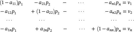
There is a balancing between the total output and the combined inputs of the product of each sector. We can show these in a set of n equations:
In this set of equations, x1, x2, ⋯xn are a set of outputs, and y1, y2, ⋯y n are the set of the final bill of goods absorbed by the economy such as households, government, industries, and so on. Combinations of the (4.12) and (4.13) make the following equations:
If we solve these equations for unknown x's, we can find the number of goods absorbed by parts of an economy are y1, y2, ⋯yn . Thus, Eq. (4.14) becomes:
For our example these equations mean total demands for x1 are combinations of all demands of these inputs in all parts of the economy, a sector y1 with its coefficient A11, plus sector y2 with its coefficient A12, and so on.
The constant Aij shows, one unit increase in xi (of the ith sector) if the yi increase in their demands. The output xi for i = j is directly affected (and also indirectly) and for i ≠ j affected indirectly. Sector j increases in their outputs, while sector i provides additional inputs for other sectors including sector j as yj. The computational view tells us each magnitude of coefficient A in the solution equations, (4.15) in general, depends on all the input coefficient a appearing on the left‐hand side of the system of equilibrium Eq. (4.14) [12].
The matrix A in the mathematical language appears as

This matrix shows the constants appearing on the right‐hand of the solution (4.15), and these constants are the inverse of this matrix:
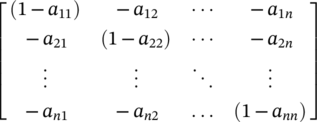
Because there are many outputs, x1, x2, ⋯xn, which are inputs for other outputs, y1, y2, ⋯yn, the inverted matrix, Aij, are nonnegative. There is a sufficient condition for this,

and of all its principal submatrices,
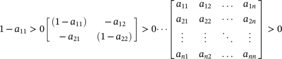
It means this matrix should be positive; this is the so‐called Hawkins–Simon condition. If this condition satisfies for one sector, then it satisfies for all other sectors, too. The material interpretation of this condition is if each sector function of an economic system absorbs the output of other sectors, directly and indirectly, it can not only sustain itself, but can also make positive delivery to final demand for smaller and smaller subsystems and so on, and this can make a sustainable production system . However, if one of them cannot pass the test, it makes abound and cause a leak that will destroy the sustainability of all systems [12].
In other words, the condition of the sustainability of an economy is the sum of the coefficients of each column and its structural matrix should be less than or equal to 1, if at least one of the column sums is less than 1 [12].
In an open economy, exports can be positive and imports can be negative for components of final demand.
4.2.5.2 Price and the Input–output Table
Another item of an economy determining an open input‐output system is price, and there are a set of equations to show the price of each productive sector of the economy. These equations consist of prices received per unit of its output and the total outlay incurred in the course of the production; these two items must be equal. The equations below show the total outlay of an economy output, these outlays include both purchases of inputs and also value‐added for other exogenous sectors [12].
In these equations, pi is the price of each product of endogenous sectors, and each of these equations describes the balance of a receiving price and payments for output. This price usually contains wages, interest on capital, and entrepreneurial revenues of households, taxes, and other final demand sectors [12].
Similar to solving Eqs. (4.14) for xi's, in these equation we solve for pi's to determine the prices of all products from the value added of each sector [12].
In Eq. (4.21) the price pi is a dependent variable of sector j with value added, vi, earned per unit of its output in sector i. In these equations too, the constant Aij measure these dependent variables, pi's [12].
There is a fantastic relationship between these two set of equations; the aij's in the rows of q. (4.14) and corresponding column of the q. (4.20) are related to each other. This means the Aij coefficients in the row of output matrix build the corresponding coefficients in the columns of the price solutions matrix, q. (4.21).
The following identity is derived from qs. (4.15) and (4.21), because of the internal consistency of the price and the quantity of relationships within an open input–output system.
This equation’s sides show two main principles of an economy. First, there are some endogenous parts of this system and exogenous parts. The left‐hand side shows paying out of endogenous parts of the system to the exogenous sectors of this system; on the right‐hand side it combines values (quantities × prices) of their respective products delivered by all endogenous sectors to the final demand. It shows the accounting identity between the receiving and spending national income.
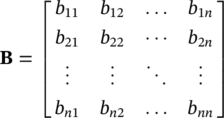
The price analysis has another viewpoint relating to the stocks used in the production processes. Stocks are a particular kind of goods such as machine tools, industrial buildings, and “working inventories” of primary or intermediate materials. These stocks are produced by industry i and employed by industry j, and measure its value based on per‐unit of the sector j output. To show this, capital requirements represent a matrix B. Each column of the matrix B describes the physical capital requirements of a particular industry. In the same way, the corresponding column of matrix A has its “current inputs” requirements [12]. The capital coefficient bij is:
The price analysis can advance by splitting the right‐hand side of the equation into two parts. The value‐added is divided into two parts: capital, invested in building, machinery, and other stocks of goods required for the production of output; and wages. In addition, there is a return on capital representing the value of all productive stocks multiplied by the given rate of return [12].
Finally, the price of goods and services has a relationship with wage rates, the rate of return on capital:
where W is a column vector of wage costs paid by different industries per unit of their respective outputs [12].
4.2.5.3 Dynamic Input–output Analysis
To describe and analyze the process of economic growth, we employ a set of linear differential equations representing dynamic input–output relationships.
In this equation, the column vector Y(t) represents the amounts of various goods and services in year t produced by sectors to households and other final users. X(t) and X(t + 1) are the column vectors representing the output levels of different industries in times t and (t+1). A is the matrix of input coefficients in Eq. (4.16), and B is the matrix of capital coefficients in Eq. (4.23). The capital stock produced in year t is used in year (t+1).
These sections are to familiarize you with the main principles of the input–output model introduced by Professor Leontief. In the following section we discuss Corrosion Economics and the input–output model by Battelle Institute, which extended these primary principles for estimating corrosion cost. To describe and analyze the process of economic growth, we employ a set of linear differential equations representing dynamic input–output relationships.
4.2.6 Depreciation, Consumption of Fixed Capital, or Corrosion
Depreciation, fixed capital consumption, or corrosion; which one is correct? The answer is ‘it depends.’ This short section shows the exact differences between these three terms.
Depreciation and CFC – In accounting terms, depreciation is used for a historical cost. The CFC is used for current value and determined by the future [11].
In the accounting system, an asset purchase finance manager calculates the asset depreciation based on a standard depreciation method. At the end of every year, the finance manager decreases that asset value without any observation in real degradation or loss. This method is used for business accounts. For example, when machinery is purchased with $2000 US and is estimated to work for 10 years with a fixed depreciation rate, its stock value will be $500 US; this calculation is:
Every year decreases the value of this machinery $150 US.
Unlike depreciation, the CFC must calculate based on the remaining benefits of a fixed asset in current prices. Computing the CFC is strict in practice because the capital that is purchased in the past must make the value in current prices as its benefits for the future.
For these reasons, depreciation as recorded in business accounts may not determine the right amount for calculation of CFC.
Depreciation and corrosion – In financial literature, these two different words are used for showing degradation in the materials. Sometimes these two words are used interchangeably, but there have some specific differences between them.
The word ‘corrosion’ derives from the verb ‘corrode,’ from Old French ‘corroder’ (14c.), and directly from Latin ‘corrodere.’ Corrodere means “to gnaw to bits, wear away,” from assimilated form of com‐ + rodere “to gnaw.” Figurative use from the 1630s [13].
The word’ depreciation’ derives from the verb ‘depreciate,’ and from the Latin word ‘depretiare.’ Depretiare means “to undervalue, under‐rate” from de “down” + pretium “price.” From the 1640s intransitive sense of “lessen the value of, to lower in value.” The intransitive sense of “to fall in value, become of less worth” is from 1790 [13].
As you can see, the word depreciation relates to the price of a substance, and the word corrosion relates to its chemical degradation. Thus, when we need to speak about the value of material we must use the term depreciation; for this reason, the financial reports use the word depreciation. Consequently; when, we speak about gnawing and chemical literature we must use the term corrosion.
4.3 Corrosion Economics
The global corrosion cost in 2013 was about 3.4% of its GDP, this percent is about $2.5 trillion per year [1]. This amount was about 77% of US gross savings and 14% of US GDP in 2013.
In economics, there are some investment models to estimate the cost of capital. These investment models design on time, the real interest rate, the capital depreciation, capital price change during the time, changes in output, tax policies, uncertainty about the future probabilities, and discount factors. These models cope with a firm investment in capital and its cost that affects the exogenous variables in the real. It also requires an infinite rate of investment [14]. These factors create complicated models that help economists to estimate economic investment and use them in their policymaking.
However, it is crucial to measure a project cost even if it is about a petrochemical refinery, but managers need the simplest and most applicable methods; these types of complicated investment models are not suitable. Thus, I bring the two most useful methods for corrosion cost measurements in this chapter.
4.3.1 Input–output Model in Corrosion
One of the most important methods for estimating corrosion cost is the input–output model (I/O). This model was introduced with Battelle Columbus Laboratories. Mr. Gordon Battelle was the founder of Battelle Memorial Institute, who lived from 1883 to 1923, and the Battelle Columbus Laboratories is one of the headquarters of the Battelle Memorial Institute. During his life, Mr. Battelle invested in lead mining and smelting operations; he later became acquainted with Professor George Waring and made a successful commercial laboratory for an economic appraisal for him [15]. The I/O method was generated with the Battelle institute in 1976 and sent to the National Bureau of Standards [16].
The I/O method applies the input–output model in economics to corrosion cost estimation. There are two broad dimensions to illustrate the I/O model. First, using and developing the input–output Leontief model, and then using three conceptual worlds for this input–output matrix. Finally, we discuss this report suggestion method for estimation of corrosion cost.
The three conceptual worlds make three scenarios for an economy; World I is an economy as it exists, World II is a hypothetical economy without corrosion, and World III is the economy with effective corrosion‐control practices. The I/O model is constructed to describe each of these economies by using its matrix.
The most significant principle in corrosion cost control is about the avoidable cost. Some of the cost is unavoidable because the gnawing is the nature of the materials. Although this cost is natural, there is some avoidable cost which can reduce it with more professional corrosion control, and the initial level for this control is familiarizing yourself with them.
As we see in the input–output of economics, we have a matrix for technical coefficients called matrix A, a matrix for capital coefficients called matrix B, and a matrix for output, X. In this section, we have three basic matrices but will divide them into their components. In the Battelle I/O method, we use the same matrices as Leontief used for his model, but the Battelle institute used it for estimation of corrosion costs, while. Leontief used it for all parts of the economy.
4.3.1.1 Matrix of Technical Coefficients
Matrix A is the matrix of direct technical coefficients. These matrix cells show the dollar worth of inputs that is required to produce one dollar of output. The worth of inputs are shown in the row, and the worth of outputs are shown in the column of this matrix. The sum of column coefficients in this matrix is inputs per dollar of its output.
To design matrix A we add three items together to obtain the matrix cells; these items are value‐added, social savings, and foreign trade. These three rows are outside the matrix A.
Value‐added is the intermediate matrix speaking about this item's nature in economics.
Social savings is a new row added to the transaction table and matrix A, and it is a hypothetical item. In World I, which is the real world, this row is empty. This item measures the labor and resources not used in the absence of corrosion; in other words, the reduction in the GNP that would take place if our world were corrosion‐free. It has an indirect influence on the sizes of all the intermediate direct coefficients [16].
Foreign trade consists of the imports of intermediate and final demand for goods and services. These imports subtend competitive and uncompetitive. The items included in the Battelle model are “noncompetitive” imports and show in the matrix as a row across the table. Because the competitive imports constitute a large proportion of the intermediate demand, these imports are not included. Demands such as crude oil contained the competitive items in this matter, for they became heavily negative total outputs [16]. To modify this problem, the Battelle carries all imports as a row outside the intermediate and inverted matrices. Thus, the total input becomes:
where TI is total input; TDI is total domestic intermediate input; DVA is domestic value added; IM is imports.
Regardless of domestic or imported, every direct coefficient in the A‐matrix is technologically correct. An import column calculates by multiplying each sector's output by the sector's import coefficient. These calculated values can add as a column to the table so that:
and
where TDO is total domestic output; TIO is total intermediate output; TFD is total final demand; TI is total inputs [16].
Finally, the column sum of the A‐matrix plus the sum of the three above items (value‐added, imports, and social savings) is equal to one since the coefficients are in terms of proportions. The sum of the column coefficients of matrix A is equal to per dollar of the output of the column sector's use of its domestic intermediate inputs.
In World I, the industry's total output is equal to the column industry's total inputs, also equal to the sum of cells of matrix and value added and import rows filling with its dollars.
4.3.1.2 Matrix of Capital Coefficients
Matrix B is the matrix of stocks used in the production processes and called the capital matrix, as you learned in the Leontief input–output model. The previous matrix, A, measures dollars worth of input per dollar of output, while B matrix measures dollars worth of capital per dollar of output. However, because there are many other definitions for the capital stock matrix, the capital matrix used in this study is for estimating this purpose.
In this matrix, the sectors listed across the top of the matrix show capital users, sectors listed across the side of the matrix indicate capital producers. There are a great many empty rows in this matrix because the capital producers are low.
Although the capital stocks excess is for more than one year and include durable goods, they need to grow and replace. The growth in the demand for an industry's output is the reference of the growing need for capital stocks, regardless of whether these growths are demand for final or intermediate goods, or foreign or domestic. In addition, capital replacement may relate to technological change or the age of existing capital. For these scenarios, matrix B changes in this manner:
where B is the standard capital coefficient matrix (expressed in the form of ratios of capital stock to output); G is matrix of annual growth rates of total capacity (capital); and R is matrix of annual replacement rates of capital.
The growth matrix – Growth in demands calls for growth in the capital matrix to determine this capacity. We need the ratio g from the first approximation growth rates of total output (X). If using K as the capacity, we use g in this manner:
We can substitute a comparable ratio based on X (which approximates capital formation change based on this total output of the sector of the economy) so that it changes approximately equal to the direct or indirect growth of general demand.
The replacement matrix – All the stock capital has a life period; this age‐structure relates to the steady growth at the rate g. In other words, the replacement rate is a function of the growth rate and the replacement life of that stock. The replacement rate (r) of each sector is a combination of both replacement life expectancy and sector growth.
Matrix of replacement lives (U) is a full matrix, like B‐matrix. Every Uij corresponding with a nonzero cell in B show a replacement life expectancy value. These values may take from a given number of years or a range of years. Each column has an average annual growth rate, gj, derived with Eq. (4.30) and used to describe the entire cycle of replacement lives.
To show the current deterioration of stock capital which has formed during a period u years, and assuming smooth growth, we must consider the reasons for growth and replacement during this period. In this sequence of years, K0 is the first year and Ku − 1 is the end of this period. The total value of the current capital stock can show as ∑K:
where K0, K1, … is the growth and replacement capital purchase in year 0,1,2, … respectively, and U is the life of first replacement of the capital stock.
Now, to obtain the annual replacement rate of capital for these sectors we have:
In a given annual growth rate of the sector g, each K becomes:
As you can see, K0 is common to all terms, thus:
Then this can transfer into:
To build the replacement matrix, R, we establish a value of rij for each corresponding value of uij.
Now is the time to set up the basic I/O model equation with recent principles together.
4.3.1.3 Input–output Model
The Leontief input–output equation can be written with this standard matrix notation:
where X is total output; A is the direct coefficient matrix; and FD is total final demand.
The rephrase of this equation says to produce the total output, so we must cover both intermediate input requirements and final demand.
Taking account of the investment demand rewrite Eq. (4.36) in this manner:
where ![]() is total capital coefficient matrix [which we saw in Eq. (4.28)]; and
is total capital coefficient matrix [which we saw in Eq. (4.28)]; and ![]() is total stipulate (noncapital) final demand.
is total stipulate (noncapital) final demand.
Thus, Eq. (4.37) can be written:
where XBG is growth capital and XBR is replacement capital, then the sum of these two terms is the total capital.
Then we extract the total output from Eq. (4.38):
4.3.1.4 Final Demand
The third major component of the I/O model is final demand. This final demand is the consumption we learned of in the first section (in estimating GDP), personal consumption, government purchases, exports, and net inventory change. In theory, the final demand summation is equal to GNP; but in reality, it needs to be adjusted. The adjustment of GNP done by adding gross private domestic investment to and subtracting imports from the consumptions.
In the final demand, the assumption is that we have full employment in the economy [16]. One of the four main concepts of economics is the employment rate. In economic principles, full employment occurs when 5% of working‐age people, aged18 to 65, are unemployed, and 95% of people are employed.
The consumption of households, government expenditure, exports, and inventory change are the four types we have discussed. In the following paragraphs, I bring these types of consumption components in the Battelle final demand.
In the Battelle approach, we have a three‐dimensional matrix for household consumption. These dimensions are income behavior class, age of head of the family, and the family size. This concept can estimate the level of consumption by a family and the entire economy as a whole [16].
For this estimation, the Battelle report designated a separate analysis to measure how families with different income and different size characteristics spend their income in certain categories.6 A regression equation expresses how many average families in a given income class spend their consumptions in one year. The total amount gathered with this method uses a PCE column in the I/O table's final demand sector. The governmental expenditure is this expenditure in the normal situation, not about the emergency programs, for example when a country is engaged in a war. Foreign trade in the final demand matrix is about the gross exports. In the A‐matrix we have a row for imports.
The last item contained in the final demand is the inventory change. It is about the change in the stock goods over many years. This issue determinate is crucial in practice; thus, economists use econometrics methods to calculate this part. In other words, the inventory change means how much goods every industry has at the end of the year in their warehouse, and this amount changes year by year. You can see this account in the table of GDP expenditure approach.
4.3.1.5 World I, World II, World III
As mentioned in the beginning of this section, there are three worlds for an economy; World I is the existing economy, World II introduce a hypothetical world without any corrosion, and World III is a hypothetical world with efficient corrosion control.
To introduce these worlds we reduce the information of World I to coefficient and range change. This means the World II and World III flow is the adjusted coefficient of World I. Adjustment of capital/output coefficient is expressed as a percentage, excess capacity for an industry, or for an entire economy; World I. Adjustment of replacement life is expressed as a change in the range of years; for example, if for World I we use 10–30 years, for World II use 20–30 years. Changes in final demands are expressed as a percentage change of World I values [16].
The differences between World I and World II is the national cost of corrosion and shows resources wasted cause of corrosion. The differences between World III and World I shows the avoidable costs of corrosion. These avoidable costs could not occur if economically preventive practices were used throughout an economy. Moreover, the differences between World III and World II measures presently unavoidable costs [17]. In all, there are differences between industries in this concept, and it relates to the users of goods and producers of goods.
4.3.1.6 Estimating Corrosion Cost by Battelle
We introduced the Battelle input/output model and described its components, in the following, we bring the Battelle models to estimate the corrosion cost in the industries.
Disaggregation – You saw in the direct technical coefficient matrix that certain cells within the final demand vectors disaggregate. This disaggregation is about the sectors producing durable goods and the corrosion prevention materials, and maintenance and repair of construction sectors. These sectors are disaggregated into corrosion‐related sectors and non‐corrosion‐related sectors. Then, we introduce some annual purchasing methods for these kinds of goods and their replacement and growth.
Social capital/infrastructure is defined as consisting of final demand of durable goods that last for more than one year.
The growth in the purchase of capital is:
where SK is social capital (in abbreviations we usually use K for capital).
Thus:
and
This equation can be rewritten in this way:
g is the growth purchases in one year, for u years this growth becomes a rate of change:
The annual replacement of social capital is:
Substituting qs. (4.44) and (4.46) into (4.40) makes:
Now solve Eq. (4.47) for (SKt) because we need to know about the social capital in time t:
Cost parameters – There are four different parameters for estimating the cost (i) the direct cost of corrosion per unit of output, (ii) the total direct costs of corrosion per sector, (iii) the direct and indirect cost of corrosion per unit of output, and (iv) the total direct and indirect cost of corrosion for each sector.
4.3.1.6.1 The Direct Cost of Corrosion per Unit of Output
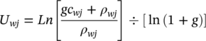
Comparing production requirements in Worlds I and II and III show the direct per‐unit cost of corrosion for each sector [16]. This production requirement is the intermediate requirement (direct technical coefficients including value‐added) per unit of the sector's output, capital requirements per unit of output of the producing sector multiplied by the sector's growth rate, and the annual replacement of capital per unit of production. These component summations show a total requirement necessary to produce a unit of a given sector's output. Below are the steps to represent the differences between these three world requirements.
Step 1. Calculate the direct requirements per unit of production:
where gj is the annual rate of growth of sector j's output; SSw,j is the social savings entry for sector j in World w (SSj is zero for World I); Cwj is the total capital/output ratio for sector j in World w; and ρwj is the total annual replacement of capital required to produce one unit of section j's output in World w.
In Eq. (4.49), 1 − SSw,j is equal to the sum of direct technical coefficients plus value‐added, and is a more direct approach to obtaining that sum.
Step 2. Calculate total direct per unit costs:
Step 3. Calculate reducible direct per unit costs:
A devised account for keeping the cost of various corrosion‐related expenses is the value SSw,j. This account contains any reductions in operating costs that those reductions relate to; both intermediate inputs and value‐added. The input changes are determined through industry surveys, and the value‐added adjustments estimated in the following ways.
Value‐added adjustments – There are several adjustments in each industry's value‐added coefficients, and it shows the differences between World I, World II, and World III. These adjustments group in the common term; Zwj. This value factors the sector j in World I (w shows the number of the world). This value Zwj is the value‐added that subtracts from sector j in World I and adds this value to row sector, SS, world w, and sector j. SS is the cumulation of net corrosion savings in the column of direct technical coefficients. Thus Zwj is defined as:
Awj shows the reduction in the cost of holding capital that the total capital requirement reduced. This occurs when the prime interest rate reflects the fact that some firms cannot obtain capital at the prime interest rate.
∆wj shows the reduction in a net accumulation of the depreciation account. Gross using of the capital and the gross accumulations in the depreciation account are measured in D. The value of replacement accounted for final demand is measured in ρ. The difference between them represents the net accumulation of in the depreciation7 account. ∆ shows the reduction in the net accumulation in World I to Worlds II and III.
ρwj represents the annual replacement of capital that is used by sector j in World w:
where rwij is the World w annual replacement rate of capital produced by sector I and used by sector j; cwij is the World w capital produced by sector I and required to produce a unit of sector j's output.
Then the average replacement rate, RRwj, can be applied to sector j's total capital:
where Cwj is the total capital/output ratio of sector j.
Referring to the replacement matrix we have:

where g is the growth rate of sector j; and U is the World w average replacement life of capital used by sector j.
Now combine qs. (4.56) and (4.57) and solve them for the average replacement life of all capital, Uwj, used by sector j:
It is not possible to calculate the straight life depreciation of capital, Dwj, owned by sector j:
4.3.1.6.2 Total Direct Costs of Corrosion
In the previous section, we estimated the cost of corrosion per output of every industry. Now, by multiplying all the outputs of every industry in that amount, we can obtain all industries corrosion costs. To obtain the differences between Worlds I and II, and Worlds I and III, you can calculate in this way too. These differences represent the total direct costs of corrosion.
4.3.1.6.3 Direct and Indirect per Unit Costs of Corrosion
We can obtain the total direct and indirect costs by calculating the total direct and indirect requirements needed to produce the vectors of direct requirements, as shown in the previous sections.
This calculation involves multiplying the vectors of direct requirements associated with each sector by the appropriate World I, II, or III inverse (the inverse in this position refers to (I − A)−1). The resulting vectors sum, and for each sector World II summation subtracts from the World I sum., then the World III summations subtract from the World I sum. Mathematically the procedure may be represented by the following steps:
Step 1. Form a Vwj of which the ith row is defined as:
where Vwij is the ith row of vector Vwj; awij is the direct technical coefficient, World w, row i, column j; gj is the growth rate for sector j; cwij is the capital supplied by sector I to sector j per unit of j's output in World w; and rwij is the annual replacement by j of capital supplied by i (capital per unit if j's output) in World w.
Step 2. Form the matrix product:
where ![]() is the inverse matrix for World w; and Xwj is the resulting output vector corresponding to sector j.
is the inverse matrix for World w; and Xwj is the resulting output vector corresponding to sector j.
Step 3. Sum columns Xwj:
where Xwij is the ith row of Xwj.
Step 4. Calculate total direct and indirect per unit cost:
Step 5. Calculate reducible direct and indirect per unit cost:
4.3.1.6.4 Total Direct and Indirect Costs of Corrosion
In these ways, we calculate the total direct and indirect costs analogous with total direct cost calculation. The outputs of steps 4 and 5 multiply by the corresponding World I sector output and show the total direct and indirect costs of corrosion.
4.3.2 Life Cycle Cost (LCC)
The life cycle of a product or service is the estimated cost in the process of their life from birth to death [18]. There have been various models for estimating cost during the years, and there is not a standard LCC model for estimation [19]. The only view in the LCC model is about cost and estimating it from all the viewpoints.
During the life cycle of a product or service, we need to consider the pre‐production, production, and post‐production costs [18]. Every system has a lifespan, and it differs from system to system. These differences include technical, economical, and usage. Annualizing the costs help to compare the different systems to each other [18]. Although as mentioned earlier, this annualizing may not reflect the actual costs, it is an acceptable method to estimate the cost of corrosion.
To modify these differences between various capitals use realistic views. Lifespan is defined as when a system begins to work, until the end of its usefulness. The cost occurring during a capital life may occur for various factors, such as insufficient maintenance during the life of the product, or those that occur naturally like hydrogeology, precipitation, temperature, and humidity. We can also include some natural disasters in nature, like floods, droughts, or hurricanes that affect the life of assets [18].
4.3.2.1 Life‐Cycle Cost Model
In the LCC model, estimation of cost sum up all the costs of a component in the lifespan and makes its life cost. This section brings two kinds of equations to use to estimate the LCC.
4.3.2.1.1 The Dr. Reddy Formulation
This equation was developed by V. Ratna Reddy and his co‐author in the “Life‐cycle Cost Approach for Management of Environmental Resources” book. This equation is quite comprehensive to show the cost of a system.
The basic functional form of the equation is:
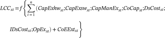
where LCCxt is life‐cycle costs of specified products/services; CapExhwxt is Capital expenditure on hardware (initial construction cost); CapExswxt is Capital expenditure on software; CapManExxt is Capital management expenditure (rehabilitation cost); CoCapxt is Cost of capital; DsCostxt is Direct support costs; IDsCostxt is Indirect support costs; OpExxt is Annual operation and maintenance cost; CoEExtxt is Cost of environmental externalities; x represents product or service, and t represents year.
This equation brings the LCC of an asset by either including the expenditure on the capital process of life or the environmental externalities8 and social sustainability. However, quantifying some of these costs is difficult to determine, as these costs must annualize for standardizing cost. Some of these costs are for the past or future; thus, we must make these costs to the PV to compare them with other investments [18]. Accordingly, Eq. (4.65) can be written as:

where pvf is present value factor (1 + r) t ; r is rate of interest or inflator and; t is time period.
Using the inflation rate or the prevailing interest rate may be appropriate for estimating the PV or worth [18].
The other view that Dr. Reddy brings is the risk based in analyzing the cost of a lifecycle. Risk and uncertainty are features of some of the components. Systems may not follow a schedule and fail randomly. Natural factors and unexpected climate events create various risk and uncertainties impressing the estimation of the component's cost.

where Psfxt is probability of risk.
This formulation is appropriate for a wet environment if the groundwater is substantial. This view of the LCC helps to estimate the real‐life cost in every climate and location [18].
4.3.2.1.2 The Professor Adeli Formulation
The other view of estimating the life‐cycle cost is from Professor Hojjant Adeli and his co‐author in the book “Cost Optimization of Structures.” They introduce a formulation for measuring the LCC of steel structure, but we can use it for any other components.
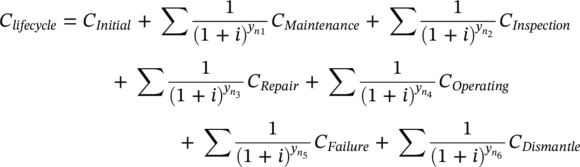
where CLifecycle, CInitial, CMaintenance, CInspection, CRepair, COperating, CFailure, and CDismantle are the total life‐cycle, initial, maintenance, inspection, repair, operating, probable failure, and dismantling costs of a steel structure, respectively; i is the discount rate of money; yn1, ![]() ,
, ![]() ,
, ![]() ,
, ![]() ,
, ![]() are the years when the associated costs incur; and ∑ denotes the summation of all the costs of the same category during the life of the structure [20].
are the years when the associated costs incur; and ∑ denotes the summation of all the costs of the same category during the life of the structure [20].
You read in the PV section that ![]() is a factor to convert the cost value to the PV discounted. These two models are two various models for estimating the cost of a life cycle in a system. In the first model, the LCC of an asset, you see system externalities, such as its effect on the climate, being profound for these estimations. In the second model, the main point is bringing all costs to the present, whether they are future or past.
is a factor to convert the cost value to the PV discounted. These two models are two various models for estimating the cost of a life cycle in a system. In the first model, the LCC of an asset, you see system externalities, such as its effect on the climate, being profound for these estimations. In the second model, the main point is bringing all costs to the present, whether they are future or past.
If you need to know about more models or estimation of the cost read the book “Life Cycle Costing for Engineers” by Professor B. S. Dhillon; in chapter 4 he introduces some LCC models and cost estimation methods.
4.4 Corrosion and Sustainability
Corrosion prevention and control is crucial for protecting public safety and the environment [21]. Although there is not the same reason for corrosion in the various areas and materials, it has a strong negative impact on its surroundings. These negative externalities reduce environmental sustainability and have a direct link to pollution in the environment and direct and indirect footprint on society by, for example, waters with chemical corroded particles or chemical the soil.
Using alloys in industries in the past years has had both positive and negative impacts on humans. One of its positive impacts is it helps with types of development and growth, but a negative one is the corrosive materials affecting our life and environment. The main reason for failing in the engineered systems is corrosion [22]. In the following, we discuss some examples of different materials and their impact on the environment and human life.
The largest corrosion threat involves nuclear industry. This industry uses zirconium alloys, and this alloy has its corrosion problems and solutions [22]. In nuclear accidents, most issues are about cooling systems and the role of water and steam. In the Three Mile Island accident in 1979, failure of the steam valve system created the accident. After two days, when the operator needed to compress the gas to the decay tanks, it was instead released into the environment. This accident has not been related to deaths or cancer threats, but increased the risk of cancer approximately 0.4%, compared with the 38–40% of all US citizens [23].
The Chernobyl accident in 1986 was the result of a flawed reactor design and operator error. The interaction of too hot fuel with the cooling water created rapid steam production and substantial damage due to design characteristics, and this accident released 5 tons of the radioactive reactor core into the environment. After this accident, 30 people died, mostly power plant employees and firemen, and about 350 000 people who lived in the surrounding areas relocated their homes. In addition, there were approximately 6500 thyroid cancer patients due to this accident [24].
In the Fukushima Daiichi Accident in 2011, following a massive earthquake, a 15‐m tsunami disabled the power supply and cooling capabilities of three Fukushima Daiichi reactors. This accident evacuated 100 000 people from their homes. Additionally, there have been 2259 disaster‐related deaths due to the consequences of this accident [25].
After reading about these dramatic accidents, you can review the table 4.7 about fixed9 and variable10 costs of nuclear power plants and compare them with other types of power plants.
Table 4.7 Power plant operation and maintenance costs in the US in 2019, by technology (2019 US dollars).
Source: www.statista.com.
| Power plant | Fixed costs | Variable costs |
|---|---|---|
| (in US dollars per kilowatt per year) | (in US dollars per megawatt hour) | |
| Biomass | 125.9 | 4.81 |
| Advanced nuclear | 121.13 | 2.36 |
| Geothermala | 113.29 | 1.16 |
| Wind; offshore | 109.54 | 0 |
| USC – 30% carbon sequestrationb | 59.29 | 10.93 |
| USC – 90% carbon sequestration b | 54.07 | 7.05 |
| Hydropower a | 41.63 | 1.39 |
| Wind | 26.22 | 0 |
| Solar photovoltaicc | 15.19 | 0 |
| Combined cycle – single shaft | 14.04 | 2.54 |
Release date: 1/1/2020; Region: United States; Survey time period: 2019 Supplementary notes:
a Cost and performance characteristics are site‐specific, so costs represent least expensive plants that can be built in the Northwest Power Pool region, where most proposed sites are located.
b USC: Ultra‐supercritical coal.
c Cost in terms of net AC power available to grid for installed capacity.
This table shows the cost consumption for 1 kW per year, the high level of cost consumption of the nuclear power plant for construction, and its need for repair and maintenance. To compare the nuclear plant with a wind or solar plant shows the justification of using solar or wind for power. Not only these types of energies are inexpensive, they are also environmentally friendly and have zero negative externality for citizens. There is no reason for using nuclear power because it is cost consuming, pollutes the environment, and threatens the citizens.
The marine and offshore industries are another industry coping with corrosion. These environments are harsh for metals and other materials. It threatens human life if one cannot use routine repair and maintenance. For example, during 1990–1991, 300 crewmembers of a ship died because the owner cut its maintenance cost and a 12 mm thick section of the ship was corroded down to 3–5 mm; corrosion was to blame for these lost lives [22]. Another example is a ship that has capsized and sank in the water; its corrosive materials cause much pollution to the sea or ocean floor. Alternately, most oil and gas factories are located offshore, and their corrosion pollutes the water and affects the inhabitants of the environment, and also threats human life when tainted seafood is consumed.
Monitoring the effect of corrosion is an interdisciplinary approach, and it seems essential for receiving sustainable development goals. This approach requires corrosion engineers, environmentalists, sociologists, and also economists. Such a group of scientists can work together toward a main goal, and bring their unique views to the subject. The sociologists search the corrosion effects on the society, the environmentalists search for the corrosion effect on nature, the corrosion managers search for the at least negative externalities of the corrosion on these two areas, and the economist can consult with them regarding what happens when all of their recommendations occur.
4.5 Conclusion
Corrosion is a global problem because it is depleting our resources, and thus needs an international effort to control it. International institutions such as the World Bank or UNDP must be included in rectifying this issue, because by considering this problem, we can help sustainable development goals with the aim of the 21st century international agencies. However, some part of this cost is unavoidable, and recent years' developments can increase the avoidable costs we saw in the 19th century. One weakness of this issue is there has been no sufficient estimation for this matter in the past 20 years. It might be one of the regular global measurements for every country, such as GDP that every country regulates to report. This regulation helps to improve corrosion management and reduce its avoidable cost.
To begin this essential effort, it needs one global agency such as UNDP to create the software with the Battelle method, then representing it to every country and getting their estimations for what can be done. Then, UNDP needs to regulate every country’s reports on corrosion annually. This type of monitoring can help to manage our resources and also help to use our materials adequately.
Because the I/O method can contain every industry of an economy, it is a suitable way for governments to estimat the corrosion cost. I suggest the government use this method; first estimate their corrosion cost annually, then try to separate the avoidable and unavoidable costs. Separating the avoidable and unavoidable corrosion costs is the initial way to manage corrosion costs. There is not a strict borderline between these two types of costs, but with some effort, these ambiguities could start to disappear. With the vast amount of corrosion depletion, it is reasonable to spend quite a bit of money on this research as a national or international project. It could reduce the avoidable cost in every country.
For some smaller projects, such as oil or gas refinery factories, it is suitable to use the LCC method. This method can measure the cost occurring while the project exists, as well as when it has finished and its future consequences. The LCC method can contain the negative externalities of a project in the environment and society; using a comprehensive LCC method is essential for receiving sustainable development goals.
Considering sustainability in the last section shows the necessity of the suitable material for several environments and industries. It can also bring some consequences for corrosion effects on the nuclear power plant industry and its negative socio‐environmental consequences. Along with its economic view, it can explain about the meaningless of this type of energy use. I think using nuclear energy relates to the politicians' requests for their purposes; they use it for generating force in other countries. Using this energy is the greatest threat to our planets’ safety. Energy policymakers must replace their policies with environmentally friendly energy, such as solar or wind. The future of energy, especially for daily energy, is for these types of energy..
4.6 Summary
“Knowledge is power;” to empower the corrosion engineers, this chapter first introduces some of the principles of economics, those an engineer needs to know for understanding the corrosion estimation methods. Then, we try to narrow down these principles to only the corrosion area. After these sections, I bring the two most common corrosion cost estimation methods; input/output, and LCC. In the I/O method, we expand on all phases of this complicated method. For the LCC method, we explain two kinds of this measurement method.
Finally, this chapter brings a short section about the corrosive materials in the industries. Although this phenomenon is one of the most eminent in today's knowledge, in this small section, I take a glance at the importance of this subject and suggest working on this view profoundly.
References
- 1 NACE International Impact (2013). Online; cited 2021 01 02. http://impact.nace.org/economic‐impact.aspx#:~:text=The%20global%20cost%20of%20corrosion%20is%20estimated%20to%20be%20US,the%20global%20GDP%20(2013).
- 2 Khabar, B.H. (2014). Online. Online; cited 2020 12 20. https://www.khabaronline.ir/news/439706/%D9%85%D9%81%D9%87%D9%88%D9%85‐%D8%B4%D9%86%D8%A7%D8%B3%DB%8C‐%DA%A9%D9%84%D9%85%D9%87‐%D9%87%D9%86%D8%B1‐%D8%AF%D8%B1‐%D9%85%D8%AA%D9%88%D9%86‐%D8%A7%D9%88%D8%B3%D8%AA%D8%A7%DB%8C%DB%8C‐%D9%88‐%D9%BE%D9%87%D9%84%D9.
- 3 Colander, D.C. (2008). Macroeconomics, 7e. New York: The McGraw‐Hill, Inc.
- 4 Navarro, P. The Power of Macroeconomics: Economic Principles in the Real World. https://www.coursera.org/.
- 5 Sachs, J. (2020). The age of Sustinable Development; cited 2020 June 15. https://www.coursera.org/learn/sustainable‐development.
- 6 Wikipedia (2020). Online; cited 2020 12 26. https://en.wikipedia.org/wiki/Alfred_Marshall.
- 7 Farmer, R.E.A. (1997). Macroeconomics. Los Angeles, CA: Roger E.A. Farmer.
- 8 Case, K.E., Fair, R.C., and Oster, S.M. (2012). Principles of Macroeconomics, 10e (ed. D. Battista). Boston, MA: Pearson Prentice‐Hall.
- 9 tradingeconomics.com. Online. cited 2020 10 11. https://tradingeconomics.com/united‐states/gdp.
- 10 Bureau of Economic Analysis (2020). Online. cited 2020 10 19. https://apps.bea.gov/scb/2020/08‐august/0820‐nipa‐update.htm#pce.
- 11 System of National Account (2008). New York: United Nations; 2009.
- 12 Leontief, W. (1986). Input‐Output Economics, 2e. New York: Oxford University Press.
- 13 The online Etymology Dictionary n.d. Online. https://www.etymonline.com/.
- 14 Romer, D. (1996). Advanced Macroeconomics (ed. L. Sutton). USA: McGraw‐Hill.
- 15 Wikipedia. Online. cited 2020 November 29. https://en.wikipedia.org/wiki/Gordon_Battelle.
- 16 Payer, J.H., Dippold, D.G., Boyd, W.K. et al.1978Economic Effects of Metallic Corrosion in the United States. A report to National Bureau of Standards. Ohio: Battelle Columbus Laboratories, U.S. Department of Commerce. Report No.: 78‐600033.
- 17 Kruger, J.E.D. and Verink, J. (2011). Uhlig's Corrosion Handbook (ed. R.W. Revie), 16–30. Pennington: Wiley.
- 18 Reddy, V.R., Kurian, M., and Ardakanian, R. (2015). Life‐Cycle Cost Approach for Managment of Environmental Resourses Dresden. Springer.
- 19 Dhillon, B.S. (2010). Life Cycle Costing for Engineers. Boca Raton, Florida: CRC Press/Taylor & Francis.
- 20 Adeli, H. and Sarma, K.C. (2006). Cost Optimization of Structures West Sussex. Wiley.
- 21 Koch, H. Brongers G.P.H. (2002). MaGTN. NACE international. Online. Dublin; cited 10/01/2021. https://higherlogicdownload.s3.amazonaws.com/NACE/cedda8a4‐c3c0‐4583‐b1b6‐3b248e6eb1f2/UploadedImages/Resources/pdf/ccsupp.pdf.
- 22 Sastri, V.S. (2015). Challenges in Corrosion Costs. New Jersey: Wiley.
- 23 World Nuclear Association (2020). Online; cited 01/10/2021. https://www.world‐nuclear.org/information‐library/safety‐and‐security/safety‐of‐plants/three‐mile‐island‐accident.aspx.
- 24 World Nuclear Association (2020). Online; cited 10/01/2021. https://www.world‐nuclear.org/information‐library/safety‐and‐security/safety‐of‐plants/chernobyl‐accident.aspx#:~:text=The%20Chernobyl%20accident%20in%201986,in%20many%20parts%20of%20Europe.
- 25 World Nuclear Association (2020). Online; cited 10/1/2021. https://www.world-nuclear.org/information-library/safety-and-security/safety-of-plants/fukushima-daiichi-accident.aspx.
Notes
- * https://www.linkedin.com/in/mahsa-mostashar-nezami-a539b578.
- 1 You can read a brief well‐writing of these heterodox approaches in the book of Macroeconomics by Professor Colander.
- 2 BEA's definition of GDI.
- 3 The system of national account is provided by the United Nations, European Commission, International Monetary Fund, Organization for Economic Cooperation and Development (OECD), and World Bank Group. The latest book published in 2008, and this information is from there. I highly recommend reading this book, you can download it for free at this URL: https://unstats.un.org/unsd/nationalaccount/sna.asp.
- 4 The “historic costs” is a name in the accounting literature for showing the value of an asset. This value is the amount of money paid in the past when the asset was purchased. In the financial reports, it shows as an asset of the units.
- 5 If you need to see these collections click the link: https://www.bea.gov/data/industries/input‐output‐accounts‐data
- 6 When the Battelle model was designed there were 42 major categories.
- 7 In my view, the account that can estimate the corrosion on the fixed capital by observation is “consumption of fixed capital account,” because the Battelle report uses this account, I write the depreciation account.
- 8 https://www.investopedia.com defines externality as: “An externality is a cost or benefit caused by a producer that is not financially incurred or received by that producer. An externality can be either positive or negative and can stem from either the production or consumption of a good or service. The costs and benefits can be both private – to an individual or an organization – or social, meaning it can affect society as a whole.” Environmental externalities are about the pollution of the air, water, or environment that occur during factory production. This is not a direct cost of the production, it's the third party of this production.
- 9 Which shows the initial cost of maintaining a nuclear power plant.
- 10 Which shows the repair and maintenance.