Philip Brisk and Majid Sarrafzadeh
As stated in Section 2.3.6 of Chapter 2, configurable processors require applications that are large enough to necessitate a complex base architecture. Portions of the application are identified as complex custom instructions using a technique such as the one described in Chapter 7. This chapter discusses the process of synthesizing a datapath that is capable of implementing the functionality of all of the custom instructions. The primary concern of this chapter is to avoid area bloat, the third major limitation of automated extension listed in Section 8.4 of Chapter 8. Techniques for resource sharing during datapath synthesis are described in detail. This work is an extension of a paper that was first published at DAC 2004 [1].
Customizable processors will inevitably be limited by Amdahl’s Law: the speedup attainable from any piece of custom hardware is limited by its utilization, i.e., the relative frequency with which the custom instruction is used during program execution. The silicon that is allocated to a datapath that implements the custom instructions increases the overall cost of the system in terms of both area and power consumption. Resource sharing during synthesis can increase the utilization of silicon resources allocated to the design. Moreover, resource sharing allows for a greater number of custom instructions to be synthesized within a fixed area.
Without resource sharing, custom instruction set extensions will never scale beyond a handful of limited operations. As the amount of silicon dedicated to custom instructions increases, the physical distance between custom resources and the base processor ALU will also increase. The interconnect structures to support such designs will increase both cost and design complexity. The next generation of compilers for extensible processor customization must employ aggressive resource sharing in order to produce area-efficient and competitive designs.
Compilers that fail to judiciously allocate silicon resources will produce designs that perform poorly and fail economically. A compiler targeting an extensible processor will generate a large number of candidate custom instructions. Most candidate generation techniques, including those in Chapter 7, are based on semiexhaustive enumeration of subgraphs of the compiler’s intermediate representation of the program.
Custom instruction selection is a problem that must be solved in conjunction with candidate enumeration. Let Candidates = {I1, I2, ..., In} be a set of candidate custom instructions. Each instruction Ij ∊ Candidates has a performance gain estimate pj and an estimated area cost aj. These values can be computed by synthesizing a custom datapath for Ij and examining the result. Custom instruction selection arises when the area of the custom instructions in Candidates exceeds the area budget of the design, denoted Amax. Amax limits the amount of on-chip functionality that can be synthesized. The problem is defined formally as follows:
Problem: Custom Instruction Selection. Given a set of custom instructions Candidates and a fixed area constraint Amax, select a subset Selected ⊆ Candidates such that the overall performance increase of the instructions in Selected is maximized and the total area of synthesizing a datapath for Selected does not exceed Amax.
A typical approach to solving this problem is to formulate it as an integer-linear program (ILP) and use a commercially available tool to solve it. A generic ILP formulation is shown next. It should be noted that many variations of the instruction selection problem exist, and this ILP may not solve each variation appropriately or exactly; nonetheless, this approach can easily be extended to encompass any variation of the problem.
Define a set of binary variables x1, x2, ..., xn, where xi = I if instruction Ii is selected for inclusion in the design; otherwise, xi = 0. The ILP can now be formulated as follows:
To date, the majority of existing solutions to the aforementioned custom instruction problem have employed either greedy heuristics or used an ILP formulation. One exception is that of Clark et al. [2], who used a combination of identify operation insertion [3] and near-isomorphic graph identification to share resources. The algorithm was not described in detail, and an example was given only for paths, not general directed acyclic graphs (DAGs).
The primary drawback of this problem formulation is that resource sharing is not considered. Area estimates are assumed to be additive. The cost of synthesizing a set of instructions is estimated as the sum of the costs of synthesizing each instruction individually. This formulation may discard many custom instructions that could be included in the design if resource sharing was used during synthesis.
As an example, consider Figs. 10.1–10.3. Fig. 10.1 shows a set of resources and their associated area costs. These resources will be used in examples throughout the chapter. Fig. 10.2 shows two DAGs, G1 and G2, representing candidate custom instructions I1 and I2. The arrows beginning with dark dots represent inputs, which are assumed to have negligible area; outputs are also assumed to have negligible area. The areas of each custom instruction are estimated to be the sum of the areas of the resources in each DAG. Then a1 = 17 and a2 = 25. Now, let Amax = 30. Then either G1 or G2, but not both, could be chosen for synthesis.
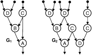
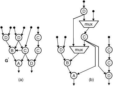
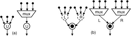
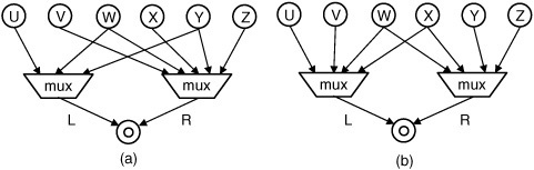
Figure 10.3. (a) G’, an acyclic common supergraph of G1 and G2; (b) a datapath synthesized from G’ that uses multiplexers to implement the functionality of G1 and G2.
Fig. 10.3 shows an alternative solution to the problem instance in Fig. 10.2. Fig 10.3(a) shows a common supergraph G’ of G1 and G2. Fig. 10.3(b) shows a datapath synthesized from G’ that implements the functionality of both G1 and G2. The area of the datapath in Fig. 10.3, once again based on a sum of its component resources, is 28. The capacity of the datapath in Fig. 10.3(b) is within the allocated design area, whereas separate synthesis of both G1 and G2 is not. Unfortunately, the custom instruction selection problem as formulated earlier would not even consider Fig. 10.3 as a potential solution. Fig. 10.3 exemplifies the folly of relying on additive area estimates during custom instruction selection. The remainder of this paper describes how to construct an acyclic supergraph of a set of DAGs and how to then synthesize the supergraph.
In Fig. 10.2, A, B, and D are binary operators and C is unary. In G3, one instance of resource B has three inputs, and one instance of C has two. Multiplexers are inserted into the datapath in Fig. 10.3(b) to rectify this situation. Techniques for multiplexer insertion during the synthesis of the common supergraph are discussed as well.
Here, we formally introduce the minimum area-cost acyclic common supergraph problem. Bunke et al. [4] have proven a variant of this problem NP-complete.
Problem: Minimum Area-Cost Acyclic Common Supergraph. Given a set of DAGs G = {G1, G2, ..., Gk}, construct a DAG G’ of minimal area cost such that Gi, 1 ≤ i ≤ k, is isomorphic to some subgraph of G’.
Graphs G1 = (V1, E1) and G2 = (V2, E2) are isomorphic to one another if there is a one-to-one and onto mapping f : V1 → V2 such that (u1, v1) ∊ E1 ⇔ (f(u1), f(v1)) ∊ E2. Common supergraph problems are similar in principle to the NP-complete subgraph isomorphism problem [5].
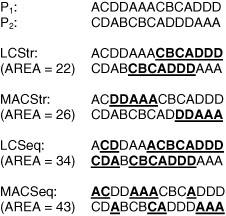
Let X = 〈x1, x2, ..., xm〉 and Y = 〈y1, y2, ..., yn〉 be character strings. Z = 〈z1, z2, ..., zk〉 is a subsequence of X if there is an increasing sequence 〈i1, i2, ..., ik〉 of indices such that:
For example, if X = ABC, the subsequences of X are A, B, C, AB, AC, BC, and ABC.
If Z is a subsequence of X and Y, then Z is a common subsequence. Determining the longest common subsequence (LCSeq) of a pair of sequences of lengths m ≤ n has a solution with time complexity O(mn/logm) [6]. For example, If X = ABCBDA and Y = BDCABA, the LCSeq of X and Y is BCBA. A substring is defined to be a contiguous subsequence. The solution to the problem of determining the longest common substring (LCStr) of two strings has an O(m + n) time complexity [7]. X and Y in the preceding example have two LCStrs: AB and BD.
If a path is derived from a DAG, then each operation in the path represents a computation that must eventually be bound to a resource. The area of the necessary resource can therefore be associated with each operation in the path. To maximize area reduction by resource sharing along a set of paths, we use the maximum-area common subsequence (MACSeq) or substring (MACStr) of a set of sequences, as opposed to the LCSeq or LCStr. MACSeq and MACStr favor shorter sequences of high-area components (e.g., multipliers) rather than longer sequences of low-area components (e.g., logical operators), which could be found by LCSeq or LCStr. The algorithms for computing the LCSeq and LCStr are, in fact, degenerate cases of the MACSeq and MACStr, where all operations are assumed to have an area cost of 1.
Fig. 10.4 illustrates the preceding concepts.
The heuristic proposed for common supergraph construction first decomposes each DAG into paths, from sources (vertices of in-degree 0) to sinks (vertices of out-degree 0); this process is called path-based resource sharing (PBRS). The sets of input-to-output paths for DAGs G1 and G2 in Fig. 10.1 are {DBA, CBA, CA} and {DBD, DBD, DCD, DCD, CCD}, respectively.
Let G = (V, E) be a DAG and P be the set of source-to-sink paths in G. In the worst case, |P| = O(2|V|); it is possible to compute |P| (but not necessarily P) in polynomial time using a topological sort of G. Empirically, we have observed that |P| < 3|V| for the vast majority of DAGs in the Mediabench [8] application suite; however, |P| can become exponential in |V| if a DAG represents the unrolled body of a loop that has a large number of loop-carried dependencies. To accommodate larger DAGs, enumeration of all paths in P could be replaced by a pruning heuristic that limits |P| to a reasonable size.
An example is given to illustrate the behavior of a heuristic that solves the minimum area-cost acyclic common supergraph problem. The heuristic itself is presented in detailed pseudocode in the next section. Without loss of generality, a MACSeq implementation is used.
Fig. 10.5(a) shows three DAGs, G1, G2, and G3, that are decomposed into sets of paths P1, P2, and P3, respectively. The MACSeq of every pair of paths in Pi, Pj, i ≠ j, is computed. DBA is identified as the area-maximizing MACSeq of P1, P2, and P3. DBA occurs only in P1 and P2, so G1 and G2 will be merged together initially. G’, the common supergraph of G1 and G2 produced by merging the vertices in the MACSeq, is shown in Fig. 10.5(b). These vertices are marked SHARED; all others are marked 1 or 2 according to the DAG of origin. This initial merging is called the global phase, because it determines which DAGs will be merged together each step. The local phase, which is described next, performs further resource sharing among the selected DAGs.
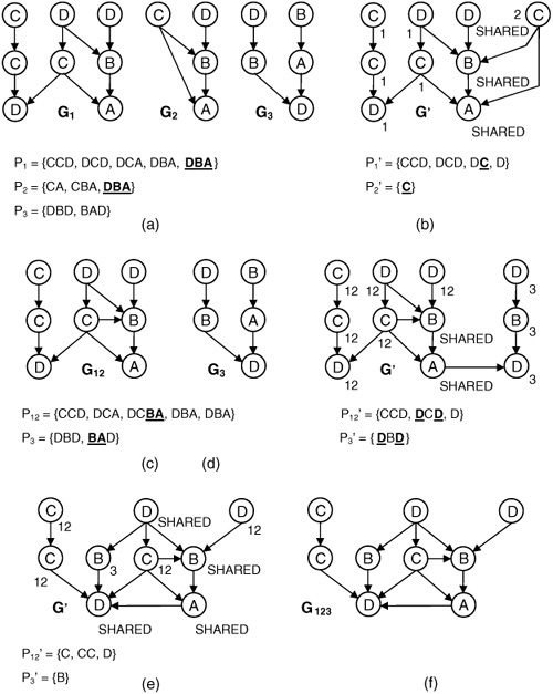
Let G1’ and G2’ be the respective subgraphs of G’ induced by vertices marked 1 and 2, respectively. As the local phase begins, G1’ and G2’are decomposed into sets of paths P1’ and P2’ whose MACSeq is C. The vertex labeled C in G2’ may be merged with any of three vertices labeled C in G1’. In this case, the pair of vertices of type C having a common successor, the vertex of type A, are merged together. Merging two vertices with a common successor or predecessor shares interconnect resources. No further resource sharing is possible during the local phase, since no vertices marked with integer value 2 remain. G1 and G2 are removed from the list of DAGs and are replaced with G’, which has been renamed G12 in Fig. 10.5(c).
In Fig. 10.5(c), the set of DAGs now contains G12 and G3. The global phase decomposes these DAGs into sets of paths P12 and P3, respectively. The MACSeq that maximizes are reduction is BA. The local phase begins with a new DAG, G’, as shown in Fig. 10.5(d); one iteration of the local phase yields a MACSeq DD, and G’ is shown after resource sharing in Fig. 10.5(e). At this point, no further resource sharing is possible during the local phase. In Fig. 10.5(f), G’ = G123 replaces G12 and G3 in the list of DAGs. Since only G123 remains, the algorithm terminates. G123, as shown in Fig. 10.5(f), is a common acyclic supergraph of G1, G2, and G3 in Fig. 10.5(a).
The heuristic procedure used to generate G123 does not guarantee optimality.
Pseudocode for the heuristic exemplified in the previous section is provided and summarized. A call graph, shown in Fig. 10.6, provides an overview. Pseudocode is given in Figs. 10.7–10.12. The starting point for the heuristic is a function called Construct_Common_Supergraph (Fig. 10.7). The input is a set of DAGs G = {G1, G2, ..., Gn}. When Construct_Common_Supergraph terminates, G will contain a single DAG that is a common supergraph of the set of DAGs originally in G.

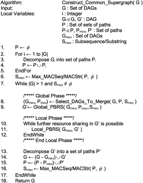
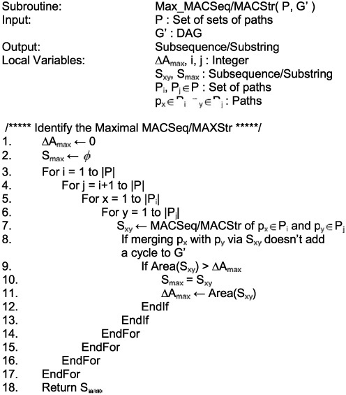
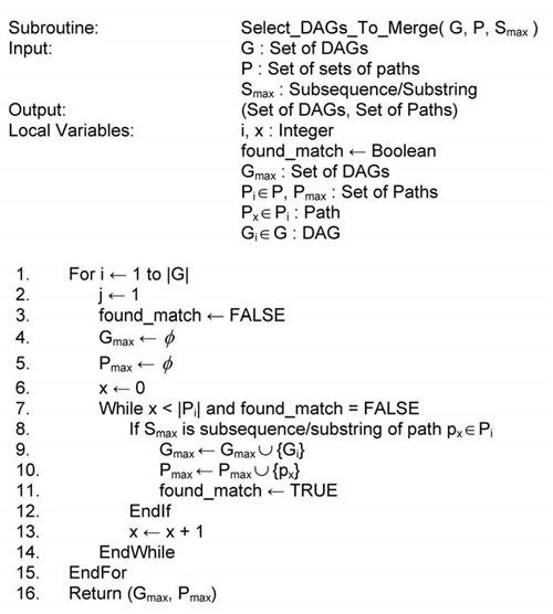
Figure 10.9. Subroutine used during the global phase to select which DAGs to merge and along which paths to initially share vertices.
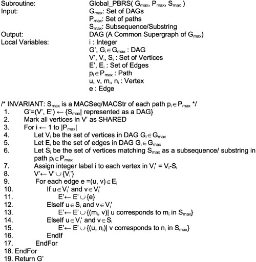

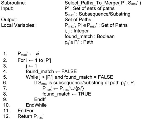
Figure 10.12. Assists Local_PBRS (Fig. 10.11) by determining which paths should be merged during each iteration.
The first step is to decompose each DAG Gi ∊ G into a set of input-to-output paths, Pi, as described in Section 10.4.1. The set P = {P1, P2, ..., Pn} stores the set of paths corresponding to each DAG. Lines 1–5 of Construct_Common_Supergraph (Fig. 10.7) build P.
Line 6 consists of a call to function Max_MACSeq/MACStr (Fig. 10.8), which computes the MACSeq/MACStr Sxy of each pair of paths px ∊ Pi, py ∊ Pj, 1 ≤ x ≤|Pi|, 1 ≤ y ≤|Pj|, 1 ≤ i = j ≠ ≤ n. Max_MACSeq/MACStr returns a subsequence/substring Smax, whose area, Area(Smax) is maximal. The loop in lines 7–17 of Fig. 10.7 performs resource sharing. During each iteration, a subset of DAGs Gmax ⊆ G is identified (line 8). A common supergraph G’ of Gmax is constructed (lines 9–12). The DAGs in Gmax are removed from G and replaced with G’ (lines 13–15).
The outer while loop in Fig. 10.7 iterates until either one DAG is left in G or no further resource sharing is possible. Resource sharing is divided into two phases, global (lines 8–9) and local (lines 10–12). The global phase consists of a call to Select_DAGs_to_Merge (Fig. 10.9) and Global_PBRS (Fig. 10.10).
The local phase consists of repeated calls to Local_PBRS (Fig. 10.11). The global phase determines which DAGs should be merged together at each step; it also merges the selected DAGs along a MACSeq/MACStr that is common to at least one path in each. The result of the global phase is G’—a common supergraph of Gmax but not necessarily of minimal cost. The local phase is responsible for refining G’ such that the area cost is reduced while maintaining the invariant that G’ remains an acyclic common supergraph of Gmax.
Line 8 of Fig. 10.7 calls Select_DAGs_To_Merge (Fig. 10.9), which returns a pair (Gmax, Pmax), where Gmax is a set of DAGs as described earlier, and Pmax is set of paths, one for each DAG in Gmax, having Smax as a subsequence or substring. Line 9 calls Global_PBRS (Fig. 10.10), which constructs an initial common subgraph, G’ of Gmax. The loop in lines 10–12 repeatedly calls Local_PBRS (Fig. 10.10) to share additional resources within G’. Lines 13–15 remove the DAGs in Gmax from G and replaces them with G’; line 16 recomputes Smax.
Construct_Common_Supergraph terminates when G contains one DAG or no further resource sharing is possible. Global_PBRS and Local_PBRS are described in detail next. Gmax, Pmax, and Smax are the input parameters to Global_PBRS (Fig. 10.10). The output is a DAG, G’ =(V’, E’), an acyclic common supergraph (not necessarily of minimal area-cost) of Gmax. G’ is initialized (line 1) to be the DAG representation of Smax as a path; i.e., Smax = (Vmax, Emax), Vmax = {si|1 ≤ i ≤|Smax|}, and Emax = {(si, si+1)|1 ≤ i ≤|Smax|– 1}. Fig. 10.10 omits this detail.
DAG Gi = (Vi, Ei) ∊ Gmax is processed in the loop spanning lines 3–18 of Fig. 10.10. Let Si ⊆ Vi be the vertices corresponding to Smax in G’. Let Gi’ = (Vi’, Ei’), where Vi’ = Vi –Si, and Ei’ = {(u, v)|u, v ∊ Vi’}. Gi’ is copied and added to G’. Edges are also added to connect Gi’ to Smax in G’. For each edge e ∊{(u, v)|u ∊ Si, v ∊ Vi’}, edge (mi, v) is added to E’, where miis the character in Smax matching u. Similarly, edge (u, ni) is added to E’for every edge e ∊{(u, v)|u ∊ Vi’, v ∊ Si}, where ni is the character in Smax matching v, ensuring that G’ is an acyclic supergraph of Gi.
All vertices in Vmax are marked SHARED; all vertices in Vi’ are marked with value i. Global_PBRS terminates once each DAG in Gmax is processed. To pursue additional resource sharing, Local_PBRS (Fig. 10.11) is applied following Global_PBRS.
Vertex merging, if unregulated, may introduce cycles to G’. Since G’must also be a DAG, this cannot be permitted. This constraint is enforced by line 8 of Max_MAC_Seq/MACStr (Fig. 10.8). This constraint is only necessary during Local_PBRS. The calls to Max_MACSeq/MACStr from Construct_Common_Supergraph (Fig. 10.7) pass a null parameter in place of G’; consequently, the constraint is not enforced in this context.
The purpose of labeling vertices should also be clarified. At each step during the local phase, the vertices marked SHARED are no longer in play for merging. Merging two vertices in G’ that have different labels reduces the number of vertices while preserving G’s status as a common supergraph. A formal proof of this exists but has been omitted to save space. Likewise, if two vertices labeled i were merged together, then Gi’would no longer be a subgraph of G’.
Local_PBRS decomposes each DAG Gi’ ⊂ G’ into a set of input-to-output paths Pi’ (lines 3–8), where P’ = {P1’, P2’, ..., Pk’}. All vertices in all paths in Pi’ are assigned label i. Line 9 calls Max_MACSeq/MACStr Fig. 10.8) to produce Smax’, the MACSeq/MACStr of maximum weight that occurs in at least two paths, px’ ∊ Pi’ and py’ ∊ Pj’, i≠j. Line 10 calls Select Paths to Merge (Fig. 10.12), which identifies a set of paths—no more than one for each set of paths Pi’—that have Smax’ as a subsequence or substring; this set is called Pmax’. Line 11 of Local_PBRS (Fig. 10.10) merges the vertices corresponding to the same character in Smax’, reducing the total number of operations comprising G’. This, in turn, reduces the cost of synthesizing G’.
Resource sharing along the paths in Pmax’ is achieved via vertex merging. Here, we describe how to merge two vertices, vi and vj, into a single vertex, vij; merging more than two vertices is handled similarly. Initially, vi and vj and all incident edges are removed from the DAG. For every edge (u, vi) or (u, vj), an edge (u, vij) is added to the DAG; likewise for every edge (vi, v) or (vj, v), an edge (vij, v) is added as well. In other words, the incoming and outgoing neighbors of vij are the unions of the respective incoming and outgoing neighbors of vi and vj.
The vertices that have been merged are marked SHARED in line 12 of Local_PBRS, thereby eliminating them from further consideration during the local phase. Eventually, either all vertices will be marked as SHARED, or the result of Max_MACSeq/MACStr will be the empty string. This completes the local phase of Construct_Common_Supergraph (Fig. 10.7). The global and local phases then repeat until no further resource sharing is possible.
This section describes the insertion of multiplexers into the acyclic common supergraph representation of a set of DFGs—for example, the transformation from Fig. 10.3(a) into Fig. 10.3(b). In the worst case, multiplexers must be inserted on all inputs for all vertices in the acyclic common supergraph. Multiplexer insertion is trivial for unary and binary noncommutative operators. For binary commutative operators, multiplexer insertion with the goal of balancing the number of inputs connected to the left and right inputs is NP-complete, per operator.
In Fig. 10.13(a), a unary operator U, assumed to be part of a supergraph, has three inputs. One multiplexer is inserted; its one output is connected to the input of U, and the three inputs to U are redirected to be inputs to the multiplexer. If the unary operator has only one input, then the multiplexer is obviously unnecessary. Now, let • be a binary noncommutative operator, i.e., a • b ≠ b • a. Each input to • must be labeled as to whether it is the left or right operand, as illustrated in Fig. 10.13(b). The left and right inputs are treated as implicit unary operators.
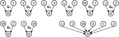
A binary commutative operator ο exhibits the property that a ο b = bοa, for all inputs a and b. The problem for binary commutative operators is illustrated by an example shown in Fig. 10.14. Eight DFGs are shown, along with an acyclic common supergraph. All of the DFGs share a binary commutative operator ο, that is represented by a vertex, also labeled ο, in the common supergraph. Consider DFG G1 in Fig. 10.14, where ο has two predecessors labeled X and Y. Since ο is commutative, X and Y must be connected to multiplexers on the left and right inputs respectively, or vice versa. If they are both connected to the left input, but not the right, then it would be impossible to compute XοY. The trivial solution would be to connect X and Y to both multiplexers; however, this should be avoided in order to minimize, area, delay, and interconnect.
The number of inputs connected to the left and right multiplexer should be approximately equal, if possible, since the larger of the two multiplexers will become the critical path through operator ο. S(k) = ⌈log2 k⌉ is the number of selection bits for a multiplexer with k inputs. The area and delay of a multiplexer are monotonically increasing functions of S(k).
Fig. 10.15 shows two datapaths with multiplexers inserted corresponding to the common supergraph shown in Fig. 10.14. The datapath in Fig. 10.15(a) has two multiplexers with 3 and 5 inputs, respectively; the datapath in Fig. 10.15(b) has two multiplexers, both with 4 inputs. S(3) = S(4) = 2, and S(5) = 3. Therefore, the area and critical delay through the datapath in Fig. 10.15(a) will both be greater than the datapath in Fig. 10.15(b). Fig. 10.15(b) is thus the preferable solution.
Balancing the assignment of inputs to the two multiplexers can be modeled as an instance of the maximum-cost induced bipartite subgraph problem, which is NP-complete [5]; a formal proof has been omitted. An undirected unweighted graph Go =(Vo, Eo) is constructed to represent the input constraints on binary commutative operator ο. Vo is the set of predecessors of ο in the acyclic common supergraph.
An edge (uo, vo) is added to Eo if both uo and vo are predecessors of ο in at least one of the original DFGs. Go for Fig. 10.14, is shown in Fig. 10.16(a). DFG G1 from Fig. 10.14 contributes edge (X, Y) to Go; G2 contributes (V, Y); G3 contributes (U, X); and so forth. Edge (uo, vo) indicates that uo and vo must be connected to the left and right multiplexers, or vice versa. Without loss of generality, if uo is connected to both multiplexers, then vo can trivially be assigned to either.
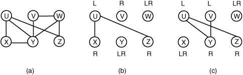
Figure 10.16. Graph Go(a), corresponding to Fig. 10.14; induced bipartite subgraphs (b) and (c) corresponding to the solutions in Fig. 10.15(a) and (b), respectively.
A solution to the multiplexer insertion problem for ο is a partition of Vo into three sets (VL, VR, VLR): those connected to the left multiplexer (VL), those connected to the right multiplexer (VR), and those connected to both multiplexers (VLR). For every pair of vertices uL, vL ∊ VL, there can be no edge (uL, vL) in Eo since an edge in Eo indicates that uL and vL must be connected to separate multiplexers; the same holds for VR. The subgraph of Go induced by VL ∪ VR is therefore bipartite. Fig. 10.16(b) and (c) respectively show the bipartite subgraphs of Go in Fig. 10.16(a) that correspond to the datapaths in Fig. 10.15(a) and (b).
The total number of inputs to the left/right multiplexers are InL = |VL| + |VLR| and InR = |VR| + |VLR|. Since VLR contributes to InL and InR, and all vertices not in VLR must belong to either VL or VR, a good strategy is to maximize VL ∪ VR. This is effectively the same as solving the maximum-cost induced bipartite subgraph problem on Go.
To minimize the aggregate area of both multiplexers, S(InL)+ S(InR) should be minimized rather than VL ∪ VR. To minimize the delay through ο, max{S(InL), S(InR)} could be minimized instead. To compute a bipartite subgraph, we use a simple linear-time breadth-first search heuristic [9]. We have opted for speed rather than solution quality because this problem must be solved repeatedly for each binary commutative operator in the supergraph.
Once the common supergraph has been constructed and multiplexers have been inserted, the next step is to synthesize the design. Two different approaches for synthesis are described here. One approach is to synthesize a pipelined datapath directly from the supergraph with multiplexers. The alternative is to adapt techniques from high-level synthesis, using the common supergraph to represent resource-binding decisions. The advantage of the pipelined approach is high throughput; the high-level synthesis approach, on the other hand, will consume less area.
The process of synthesizing a pipelined datapath from a common supergraph with multiplexers is straightforward. One resource is allocated to the datapath for each vertex in the supergraph. Pipeline registers are placed on the output of each resource as well. For each resource with a multiplexer on its input, there are two possibilities: (1) chain the multiplexer together with its resource, possibly increasing cycle time; and (2) place a register on the output of the multiplexer, thereby increasing the number of cycles required to execute the instruction. Option (1) is generally preferable if the multiplexers are small; if the multiplexers are large, option (2) may be preferable. Additionally, multiplexers may need to be inserted for the output(s) of the datapath.
Pipelining a datapath may increase the latency of an individual custom instruction, since all instructions will take the same number of cycles to go through the pipeline; however, a new custom instruction can be issued to the pipeline every clock cycle. The performance benefit arises due to increased overall throughput. To illustrate, Fig. 10.17 shows two DFGs, G1 and G2, a supergraph with multiplexers, G’, and a pipelined datapath, D. The latencies of the DFGs are 2 and 3 cycles, respectively (assuming a 1-cycle latency per operator); the latency of the pipelined datapath is 4 cycles.

High-level synthesis for a custom datapath for a set of DFGs and a common supergraph is quite similar to the synthesis process for a single DFG. First, a set of computational resources is allocated for the set of DFGs. The multiplexers that have been inserted into the datapath can be treated as part of the resource(s) to which they are respectively connected.
Second, each DFG is scheduled on the set of resources. The process of binding DFG operations to resources is derived from the common supergraph representation. Suppose that vertices v1 and v2 in DFGs G1 and G2 both map to common supergraph vertex v’. Then v1 and v2 will be bound to the same resource r’ during the scheduling stage. This binding modification can be implemented independently of the heuristic used to perform scheduling.
The register allocation stage of synthesis should also be modified to enable resource sharing. The traditional left edge algorithm [10] should be applied to each scheduled DFG. Since the DFGs share a common set of resources, the only necessary modification is to ensure that no redundant registers are inserted as registers allocated for subsequent DFGs. Finally, separate control sequences must be generated for each DFG. The result is a multioperational datapath that implements the functionality of the custom instructions represented by the set of DFGs.
To generate a set of custom instructions, we integrated an algorithm developed by Kastner et al. [11] into the Machine SUIF compiler framework. We selected 11 files from the MediaBench application suite [8]. Table 10.1 summarizes the custom instructions generated for each application. The number of custom instructions generated per benchmark ranged from 4 to 21; the largest custom instruction generated per application ranged from 4 to 37 operations; and the average number of operations per custom instruction for each benchmark ranged from 3 to 20.
Table 10.1. Summary of custom instructions generated
Exp | Benchmark | File/Function Compiled | Num Custom Insts | Largest Instr (Ops) | Avg Num Ops/Instr |
|---|---|---|---|---|---|
1 | Mesa | blend.c | 6 | 18 | 5.5 |
2 | Pgp | Idea.c | 14 | 8 | 3.2 |
3 | Rasta | mul_mdmd_md.c | 5 | 6 | 3 |
4 | Rasta | Lqsolve.c | 7 | 4 | 3 |
5 | Epic | collapse_pyr | 21 | 9 | 4.4 |
6 | Jpeg | jpeg_fdct_ifast | 5 | 17 | 7 |
7 | Jpeg | jpeg_idct_4×4 | 8 | 12 | 5.9 |
8 | Jpeg | jpeg_idct_2×2 | 7 | 5 | 3.1 |
9 | Mpeg2 | idctcol | 9 | 30 | 7.2 |
10 | Mpeg2 | idctrow | 4 | 37 | 20 |
11 | Rasta | FR4TR | 10 | 25 | 7.5 |
Next, we generated a VHDL component library for a Xilinx VirtexE-1000 FPGA using Xilinx Coregen. We converted the VHDL files to edif netlists using Synplicity Synplify Pro 7.0. Each netlist was placed and routed using Xilinx Design Manager. Table 10.2 summarizes the component library.
Table 10.2. Component library
Component | Area (Slices) | Latency (cycles) | Delay (ns) | Frequency (MHZ) |
|---|---|---|---|---|
adder | 17 | 1 | 10.669 | 93.729 |
subtractor | 17 | 1 | 10.669 | 93.729 |
multiplier | 621 | 4 | 10.705 | 93.414 |
shifter | 8 | 1 | 6.713 | 148.965 |
and | 8 | 1 | 4.309 | 232.072 |
or | 8 | 1 | 4.309 | 232.072 |
xor | 8 | 1 | 4.309 | 232.072 |
not | 8 | 1 | 3.961 | 252.461 |
2-input mux | 16 | 1 | 6.968 | 143.513 |
4-input mux | 32 | 1 | 9.457 | 105.742 |
We tested both MACSeq and MACStr implementations of the common supergraph construction heuristic in Section 10.4.3. In virtually all cases, the MACSeq was, coincidentally, a MACStr. Results are only reported for the MACSeq implementation.
To synthesize the custom instructions, the two approaches described in Section 10.6 were used. The first approach synthesized the common supergraph (following multiplexer insertion) using a high-level synthesis and floorplanning system developed by Bazargan et al. [12] and Memik et al. [13] with modifications as discussed in Section 10.6.2. The second synthesizes a pipelined datapath as discussed in Section 10.6.1. The first approach will lead to an area-efficient design, whereas the second is designed for raw performance. These experiments demonstrate the importance of resource sharing during custom instruction set synthesis and datapath generation. Area results for the 11 benchmarks that we tested are presented in terms of slices.
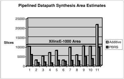
Fig. 10.18 presents results using high-level synthesis. The columns labeled Additive show the area that would result from synthesizing each custom instruction individually; the columns labeled PBRS show the area of synthesizing the set of DFGs using the common supergraph to perform binding, as discussed in Section 10.6.2. The Xilinx VirtexE-1000 FPGA has a total area of 12,288 slices; this value is shown as a horizontal bar.

PBRS reduced the area of the allocated computational resources for high-level synthesis by as much as 85% (benchmark 4) relative to additive area estimates. On average, the area reduction was 67%. In the case of benchmark 11, the additive estimates exceed the capacity of the FPGA; PBRS, on the other hand, fit well within the design. Clearly, sharing resources during custom instruction set synthesis can reduce the overall area of the design; conversely, resource sharing increases the number of custom instructions that can be synthesized within some fixed area constraint. Resources are not shared between DAGs that are synthesized separately in the additive experiment. An overview of resource sharing during high-level synthesis can be found in Di Micheli’s textbook [14].
Fig. 10.19 shows the results for pipelined datapath synthesis. For each benchmark, the area reported in Fig. 10.19 is larger than that reported in Fig. 10.18. Pipeline registers were inserted into the design during pipelined datapath synthesis; this is a larger number of registers than will be inserted during high-level synthesis. Second, the resource sharing attributable to high-level synthesis has not occurred. We also note that the results in Fig. 10.18 include floorplanning, while those in Fig. 10.19 do not. For pipelined datapath synthesis, PBRS reduced area by as much as 79% (benchmark 4) relative to additive area estimates; on average, the area reduction was 57%. Benchmark 6 yielded the smallest area reductions in both experiments. Of the five instructions generated, only two contained multiplication operations (in quantities of one and three, respectively). After resource sharing, three multipliers were required for pipelined synthesis and two for high-level synthesis. The area of these multipliers dominated the other elements in the datapath.
During pipelined synthesis, the introduction of multiplexers into the critical path may decrease the operating clock frequency of the system. This issue is especially prevalent when high clock rates are desired for aggressive pipelining. Some clock frequency degradation may be tolerable due to multiplexer insertion, but too much becomes infeasible. When multiplexers are introduced, we are faced with two options: store their output into a register, thus increasing the latency of every customized instruction by 1 cycle per multiplexer, or, alternatively, chain the multiplexer with its following operation, reducing clock frequency. To avoid the area increase that would result from inserting additional registers, we opted for a lower operating frequency. In only one case, a multiplexer required three selection bits; all other multiplexers required one or two selection bits, the vast majority of which required one.
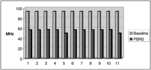
Fig. 10.20 summarizes the clock degradation observed during pipelined datapath synthesis. The baseline frequency is the highest frequency supported by the multiplier, the limiting component in the library in Table 10.3. The PBRS frequency is the frequency at which the pipeline can run once multiplexers have been inserted into the datapath. The PBRS frequency ranged from 49.598 MHz (Exp. 5) to 56.699 MHz (Exp. 3 and 10). The variation observed in the final frequency column depends on the longest latency component that was chained with a multiplexer and the delay of the multiplexer. For example, if a multiplier (delay 10.705 ns) is chained with a 2-input multiplexer (delay 6.968 ns), the resulting design will run at 56.583 MHz.
The area and clock frequency estimates presented here were for the datapath only, and did not include a control unit, register file, memory, or other potential constraining factors in the design. One cannot assume that the frequencies in Table 10.2 represent the clock frequency of the final design. The baseline frequency is overly optimistic, because it is constrained solely by the library component with the longest critical path delay—the multiplier. Additionally, retiming during the latter stages of logic synthesis could significantly improve the frequencies reported in Fig. 10.20; this issue is beyond the scope of this research. It should also be noted that multipliers had a significantly larger area than all other components. None of the benchmarks we tested required division or modulus operations, which are likely to consume even larger amounts of chip area than multipliers. Consequently, designs that include these operations will see even greater reductions in area due to resource sharing than the results reported here.
As the experimental results in Section 10.7 have demonstrated, failure to consider resource sharing when synthesizing custom instruction set extensions can severely overestimate the total area cost. Without resource-sharing techniques such as the one described here, customization options for extensible processors will be limited both by area constraints and the overhead of communicating data from the processor core to the more remote regions of the custom hardware.
A heuristic procedure has been presented that performs resource sharing during the synthesis of a set of custom instruction set extensions. This heuristic does not directly solve the custom instruction selection problem that was discussed in Section 10.2. It can, however, be used as a subroutine by a larger procedure that solves the custom instruction selection problem by enumerating different subsets of custom instructions to synthesize. If custom instructions are added and removed from the subset one by one, then the common supergraph can be updated appropriately by applying the heuristic each time a new instruction is added. Whenever a custom instruction is removed, its mapping to the supergraph is removed as well. Any supergraph vertex that has no custom instruction DAG vertices that map to it can be removed from the supergraph, thereby reducing area costs. In this manner, the search space for the custom instruction selection problem can be explored. The best supergraph can be synthesized, and the corresponding subset of custom instructions can be included in the extensible processor design.