Chapter 5

Data Model Components

The next day I started in with Luke to define some of the major components of data models. The first major topic for Luke was uniqueness.I had the opportunity to work briefly with Ted Codd at IBM in the late 1970s. I thought it would be good to get in some name dropping to increase my “cool factor” with Luke. Unfortunately he had never heard of Ted and therefore was unimpressed with my brief but educational encounter with the founder of my discipline. Ted Codd, the inventor of relational data modeling and the SQL programming language, said that uniqueness was one of the most important issues in data modeling. He said that we can understand and evaluate the real world because our brains can distinguish one thing from another thing.

For example, people are built by their DNA to have unique facial characteristics, and our eyes and brains are built by our DNA to recognize each person uniquely. This allows us to know specifically who is helping us and who is not helping us and then reciprocate appropriately. In our caveman days, reciprocation for not helping was usually implemented with a club to the head. Today, we tend to see more dialog, compromise, forgiveness, and collaboration. Well, uh, at times…

If our computing systems are going to understand and evaluate, they must have the same ability to distinguish one thing from another thing.

Uniqueness Constraints

Uniqueness constraints are how we distinguish one thing from another thing in a data model and in a physical database. I asked Luke to pick an entity and tell me what attributes are required to uniquely identify instances of that entity. He picked the entity Person, a particularly slippery species when it comes to unique identification in data models. I got Luke to go to the whiteboard and list the attributes necessary to uniquely identify persons.

• He started with the typical suspects like:
• First Name
• Last Name
• Address
• Phone Number

I, of course, pointed out that two Bill Smiths can live in the same apartment and share a single landline for phone calls. In that case, the data model can store the first Bill Smith, but when his roommate Bill Smith comes along, the uniqueness constraint will stop him from entering the system. Stumped for the moment, Luke renewed his attack. He tried Social Security number (SSN). I asked for his Social Security number, and he admitted that he does not have one. This realization triggered a related thought that when he has his own business, legally I owe him his own SSN.

Now that both uniqueness attempts failed, he regrouped for another try. How about biometric measures of people like facial geometry, retina shape, fingerprint, or DNA? Yes, in certain business contexts, these are great attributes for uniqueness of Person. Luke asked for me to elaborate on “business contexts,” and, being verbose, I gladly obliged.

To uniquely identify a Person, the context could be the level of security needed. High-security person identification needs, such as for handling nuclear waste disposal, may require biometric measures such as fingerprint, retina pattern, facial geometry, and DNA. Medium-security person identification needs, such as for purchasing software on the web, may require identity authentication such as through a Facebook account, Windows Live email account, etc. Low-security person identification needs, such as a Boy Scout recruiting sign up on a paper form at school event, may require user-supplied attributes such as first name, last name, address, phone number, and birth date.

Luke was able to see that depending on what you were trying to do, the information required could be very different. Unique keys can have different owners. Some keys are created by the business, and some keys are created by the computing system. Business keys are typically text or date data types. System keys are typically numeric.

When the data modeler has multiple unique keys on a single entity, she must choose one and only one key as the primary key; all other unique keys become alternate keys. Below is a uniqueness example for the entity Taxpayer.

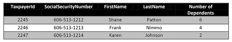
A system key is a field containing a number that is generated by the system. In order to maintain uniqueness, no two rows in the same entity will ever have the same number. It is frequently a running sequence number that just keeps getting bigger as more rows are added. The TaxpayerId in the above example is a system key.

A natural key is an attribute of the entity that happens to be unique across all rows. For example, Social Security Number is unique to each individual, so if it were legal to do so, it could be used as a unique identifier for a Person (given system scope of US citizens).

It is often preferable to have a system key that is used internally by the system while also having a business key that is visible to and used by business users. When a natural key exists, it makes sense to use it as the business key. So the system would use TaxpayerId behind the scenes, while the business user of the system would see SocialSecurityNumber. Now one of those attributes must be picked as the primary key and the other must become the alternate key.

A primary key is the identifier that will be used to identify each unique record in an entity/table. An alternate key is an attribute/column in the same entity/table that could also be used to uniquely identify the record. All of the attributes/columns that could uniquely identify a record are called candidate keys. One is chosen to be the primary key and the others are alternate keys

The LDM should use the natural key as the primary key when only one exists. Where multiple natural keys exist, select the one that is the most stable (least likely to be updated). For this LDM, the primary key would be the Social Security number, and the Taxpayer Id would be the alternate key or left out completely. In the physical data model, the Taxpayer Id will be the primary key, and the Social Security number will become an alternate key. This is done so that if the natural key is changed, it will be changed in one and only one entity or table. Business users cannot change the Taxpayer Id since it is maintained behind the scenes and they are not aware of its existence.

Key Points

• Being able to discriminate one thing from another thing is a critical capability for both humans and computing systems to be successful.
• Uniqueness in the system that mirrors uniqueness in the real world is mandatory for computing system success.
• Things are unique while at the same time they are interdependent due to entity to entity relationships.

Relationships

Relationships are built in a data model by copying the primary key of an entity to become a foreign key in a neighboring entity. Each entity has a primary key that identifies unique instances within the entity. For example, Social Security number could be the primary key to entity Taxpayer. The neighbor entity called Taxpayer Filing is the history of a given taxpayer submitting his tax statement. The Social Security number in the Taxpayer Filing entity is called a foreign key.

Relationships are the silken strands that create a web of entities. This structure represents the pathways for traversing the data that are available to the consumers of the data.

Luke stopped me. His scrunched up forehead had confusion written on it, so I backed up and gave some examples. I went to my car and pulled out the auto club map of Florida. I asked Luke a silly question, “When we go from Jacksonville to Gainesville, how do we do it?” He replied that we travel on highway 412 East for about an hour. “OK. If we consider each city to be an entity and each highway to be a relationship, then this map of Florida is built like a data model is built. We traverse from city to city using the roads, and we traverse from entity to entity using the relationships.”

Luke pulled out his cell phone and turned on his driving directions app. This app uses the Global Positioning System and a database of cities and highways. He asked if this driving directions database was an example of my example. Yes, he was correct. The driving directions app traverses the relationships in the database to find the optimal pathway for us to travel. Then we physically traverse the roads under the surveillance of GPS. Once again I was stunned to see him understanding my lesson to the point of applying it to the next layer of utility on his cell phone app. Luke sat in silence for a moment and then announced that he was ready to start his Relationship lecture. So I continued.

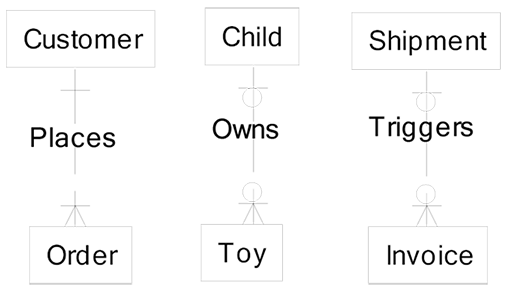
Each relationship has a purpose. Relationships are named with verb phrases to describe the nature of the relationship between the two entities being related. For example, Entity1 (verb) Entity2, so in the following diagram, Customer (places) Order, Child (owns) Toy, and Shipment (triggers) Invoice:

Referential integrity rules define how a collection of entities or tables are tied together to create a structure that can be traversed along the relationship pathways. Creating a relationship between two entities means that the primary key (PK) attributes of the entity where the relationship starts (parent entity) will be added to the entity where the relationship ends (child entity). These attributes are called a foreign key (FK) because they are not native to the entity and appear in the child entity because they have migrated via the relationship from the parent entity.

Identifying vs. Non-identifying Relationships

In identifying relationships, the parent entity PK migrates to the child entity and becomes part of its PK. To identify unique instances of the Room child entity, I must know the Building parent entity that houses the room.

Non-identifying relationships have the parent entity PK migrating to the child entity, but not as part of the child PK. To identify unique instances of Computer Equipment, I do not need to know the Building Id and Room Number where it happens to be sitting at the moment.

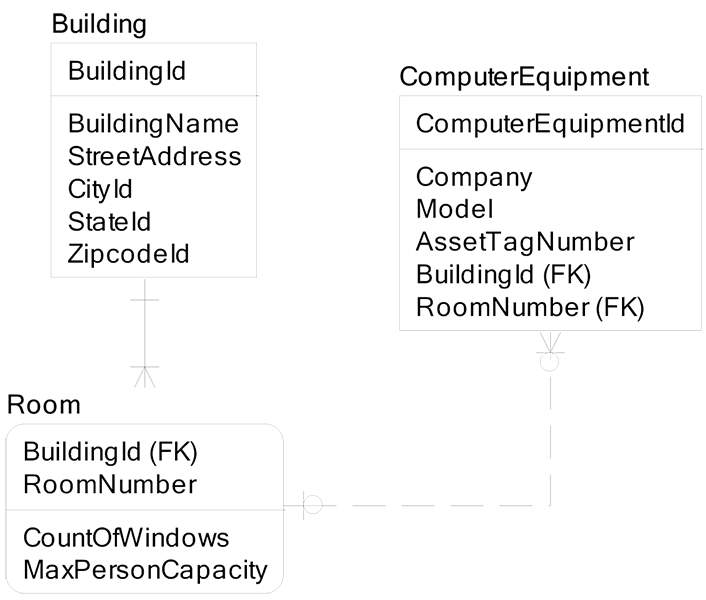
Attributes above the line are PK attributes. Building has an identifying relationship to Room (solid line). Room has a non-identifying relationship to Computer Equipment (dashed line).

• A Building can have one or more Rooms, so zero Rooms is not a possibility for a Building. A Room must be in a Building.
• A Room can have zero, one, or more Computer Equipment. A Room can be identified independent of the Computer Equipment in the Room at any moment. Computer Equipment can have one or zero Rooms. Computer Equipment can be identified independent of the Room where it sits at any moment.

Not Null FK means the relationship is mandatory, and all children must have the parent. Nullable FK means that a child can exist and not have the parent. In the example above, Computer Equipment (child) may or may not have a Room (parent), so BuildingId and RoomId can be null attributes in the Computer Equipment entity.

Relationships are specified by this list of set intersection conditions:

• Zero, one, or more
• Zero or one
• One or more
• Exactly x

In the example of identifying relationships on the previous page, each Building has a Building Id, each Room has a Room Number, and every Building must have at least one Room. A Building with no Rooms is not a Building that my business cares to record, so there will be no rows in the Room entity with a null Building Id. This is due to the primary key rule that no part of a primary key can be missing or null. This means that when I insert a new Room row, the Building Id must be present. For you and me to meet at the right place for lunch today, I need to tell you both the Room Number and the Building Name. If I just say meet in Room 1233, then you may well go to the wrong building to meet me. I must say meet me in the Smith Towers Building in Room 1233 for lunch today. The three identifying relationship types are below, starting left to right:

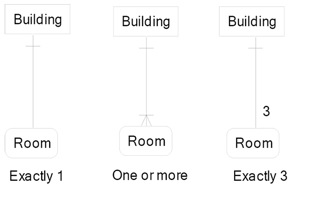
1. A Building must have one Room. A Room must always have one and only one Building.
2. A Building must have at least one Room and can have many Rooms. A Room must have one and only one Building.
3. A Building must have three Rooms. A Room must have one and only one Building.

I don’t know of any businesses that actually have rules to limit their buildings to one or three rooms. The data model below shows identifying relationships that happen far more frequently. Read data model from left to right:

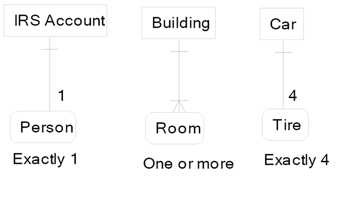
1. An IRS Account must have one Person. A Person must have one and only one IRS Account.
2. A Building must have a least one Room and may have many Rooms. A Room must have one and only one Building.
3. A Car must have four Tires. A Tire must be on one and only one Car.

In non-identifying relationships, attributes of a foreign key may be null. This was not true for the identifying examples above, where a null foreign key value was disallowed. In the examples below, every Toy may or may not belong to a Child. Also, I can identify a Child without any knowledge of Toys. Conversely I can identify Toys without any knowledge of the Child that owns the Toy.

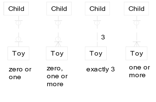
Of course Luke disliked most of these non-identifying relationship types. This is Luke’s list of most hated relationship types reading from left to right:

1. Zero or one Toys for each Child (hates it; at most one toy can exist, and zero toys is possible)
2. Zero, one, or more Toys for each Child (dislikes zero as still being possible, one is lame, and more is the only hopeful sign)
3. Exactly three Toys for each Child (feels uneasy with just three, but is glad that zero, one, or two toys is impossible)
4. One or more Toys for each Child (happy that zero is impossible and more than three is possible)

One-to-Many Relationships

Luke wanted to data model people and baseball tickets since we recently attended a pre-season professional game. So we did a data model of Person and Baseball Ticket. Luke insisted on specifying the referential integrity rules for the relationship between a person and a baseball ticket. Here is the model and a description of each rule appears below the model:

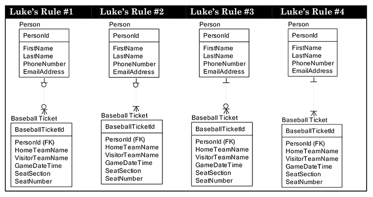
• Luke’s Rule #1: A Person may have no Tickets and a Ticket may have no Person in the model below. This is indicated by the circle near baseball ticket, meaning a person may have no ticket. The circle near the person means that a ticket can have no person.
• Luke’s Rule #2: Then Luke said that he wants every Person to always have a Ticket, so I removed the O from the baseball ticket side of the relationship and added a bar, meaning the person must have at least one ticket to be created in this data model.
• Luke’s Rule #3: Then Luke said, “No, I meant to say that I want every ticket to always belong to a person, and a person can exist with no tickets.”
• Luke’s Rule #4: Then, just to aggravate me, he said, “No, I meant to say that every ticket has to belong to a person, and every person has to have a ticket,” so I calmly changed the model again.

Many-to-Many Relationships

I let Luke pick the topic of this modeling section. He selected his hobbies and friends as the scope statement for our many-to-many data modeling lesson. I asked the following questions of Luke: “For a given Friend, say Cyrus, how many hobbies can you play with him?” He responded that Cyrus plays basketball and badminton. “For a given Hobby, say basketball, how many friends play this hobby?” He responded, “I play basketball with Cyrus, Aden, and Tristan.”

Luke got up to the whiteboard and fished around to data model this project using two entities. No matter how he tried, it failed. I suggested he try modeling this problem with three entities and voila, it worked. His finished data model is below:

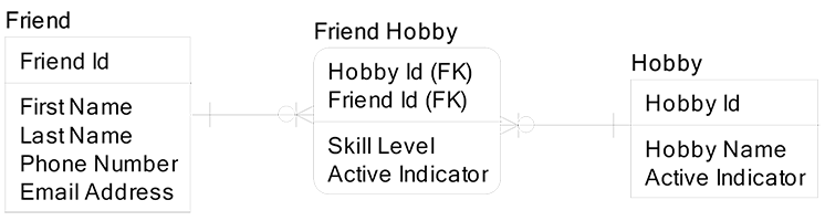
The entity in the middle is called either a many-to-many associative entity or an intersection entity; the terms are synonymous. I asked Luke to explain his data model, so he stated: A friend may stop doing a hobby that I am still doing, so the Active Indicator in the entity Friend Hobby tells us if a friend is still engaging in the hobby. An inactive friend for a hobby may suddenly become active, so we’d flip his Active Indicator back on. Further, I may choose to stop participating in some hobby for some period of time, so I can set the Active Indicator in the Hobby entity to falsely to show that I no longer do this hobby. If I chose to restart the Hobby, I still have a record of all my Friends who formerly played the hobby with me.

I requested that we put an Active Indicator in the Friend entity, so he can un-friend his friends. Then I suggested we just delete the row for that Friend when he wants to un-friend a former Friend. Luke properly pointed out that a physical delete would not allow him to easily change his mind and re-friend his formerly un-friended friend while retaining all the information about that friend and his hobbies. So I agreed, and we added the Active Indicator attribute to the Friend entity. As a general rule, the Active Indicator attribute applies to most entities.

Recursive Relationships

Recursive relationships are another topic I was worried that Luke might not be ready to understand. Recursive relationships exist when the rows of an entity relate to other rows in the same entity. For example, some Product rows are related to other Product rows. I told Luke the real-life story of my first recursive encounter:

As a boy of about four years old, I awoke late one Saturday morning to the call of breakfast on the table. I sat down half asleep and grabbed a box of cereal. I looked at the front of the box hoping to find my favorite sugar-laden brand, but found a new healthy cereal instead. On the front of the box was a picture of a baseball player holding a box of the cereal, and, of course, on the small box he was holding was an even smaller baseball player holding an even smaller box, etc. Well, I had the strangest sense of tumbling head over heels, as I felt like I was falling in slow motion into the picture on the front of the box. I closed my eyes to make the sensation stop, but I continued falling into the black hole of recursion. My mom saw my troubled look and asked if I was okay. I opened my eyes and was glad to see that I was still outside of the box, firmly anchored into my chair. I was relieved to still be full size and was glad to have stopped tumbling into the picture. I was fully awake by now, felt a bit shaky, and had lost my appetite.

Luke asked me if I had seen Alice in Wonderland when she fell down the rabbit hole. Come to think of it, I had seen that movie at about the time. I warned Luke to never take his children go see Alice in Wonderland followed by exposure to recursion. Luke replied that he would have no children since fifth grade girls were so yucky that marriage was too disgusting to consider possible. I suggested that his views will change with his hormones, but he rejected my prediction. Luke shook his finger at me saying, “Dad, you are old fashioned. You don’t understand fifth grade girls these days.”

Meanwhile, old-fashioned Dad and new-fashioned Luke were not progressing on his recursion lesson, so I continued. Recursive relationships exist in two types:

1. One-to-Many Recursive Relationships
2. Many-to-Many Recursive Relationships

First, for one-to-many recursive relationships, the classic example is the military hierarchy:

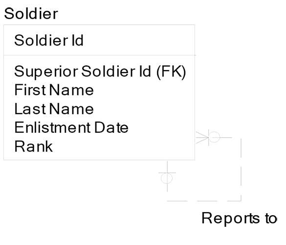
Each soldier row has one and only one row in the Soldier entity. Each also has one and only one value in the attribute Superior Soldier Id. This means that each soldier reports to one and only one superior. Each superior can have many subordinate soldiers, since the foreign key attribute of Superior Soldier Id is not unique in the entity. If I am a General and my Soldier Id is 344, and if I have three subordinates, then the attribute Superior Soldier Id will have three rows with the value 344 for my three subordinates Frank, Bruce, and John:

The top soldier has a null value for his row in the attribute Superior Soldier Id. This top soldier may report to the President, who is a civilian and is not in the Soldier entity.

Luke requested that we data model the topic of families using one-to-many recursion, but we could not do this since each child has many parents, and the rule for one-to-many recursion is that each subordinate has one superior. So one-to-many recursion cannot model families, but Luke’s suggestion indicated his brain was tracking the concept of recursion.

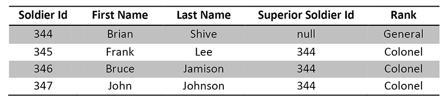
This led us to many-to-many recursive relationships. In many-to-many recursion, we need to introduce the ideas that one child can have many parents and one parent can have many children. Data modeling a simple thing like a family is surprisingly difficult, with dozens of valid design options and no clear winner for all business contexts. Other seemingly complex things like manufacturing can be surprisingly easy to data model with clear winners and losers. Below is one data model for Family. The entity Family Structure is a many-to-many recursive associative entity.

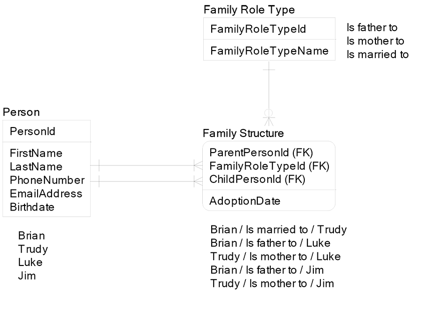
The model above allows for polygamy (one man has many wives). To avoid breaking the law, the data model can use one-to-one recursion for marriage to disallow polygamy, as shown below:

Now each Person row can have one and only one Married To Person Id value, so we conform to the polygamy laws. Also, each child can have many parents and each parent can have many children.

There are two unique constraints on the Person entity above:

• Person Id attribute is unique
• Married To Person Id is unique, when present

This is how we get one husband and one wife enforced using one-to-one recursion. For single people, the Married to Person Id is null. Luke was lost in the clouds that often obscure the topic of recursion, so I thought it best to wrap up the topic and bike to the park.

We would return to attempt to scale the Mount Everest of recursion by climbing the concept of many-to-many recursive relationships. There exists a process called many-to-many recursion explosion. This process starts with an entry point and finds related rows that are chained to the entry point. For example, an explosion of the Person and Family entities could start with Person = Brian Shive as the seed condition, and then traverse neighboring links to find all rows related to Brian Shive. The explosion traversal rules could include:

• Just my children
• Just my parents
• Both my children and my parents
• Just my grandparents
• Both my grandparents and my parents
• Both my grandparents and my children

…lots of traversal routes possible…You can fall into the rabbit hole following many pathways.

Luke demanded a break from the lecture, so we went out on the deck and had some hot chocolate and toast. I told Luke that we would resume shortly and he could pick the topic for our final recursion lesson. Luke had recently enjoyed disassembling our broken toaster. He asked for a recursion lesson on toasters, so we returned to our lesson with toasters in our sights.

The classic example of directed graph traversal is Bill of Materials for Products. If I design my products using Part Numbers in a many-to-many recursive structure, I can easily find the total quantity of Part Numbers that need to be ordered to support my factory. In the example below, I am designing and manufacturing toasters.

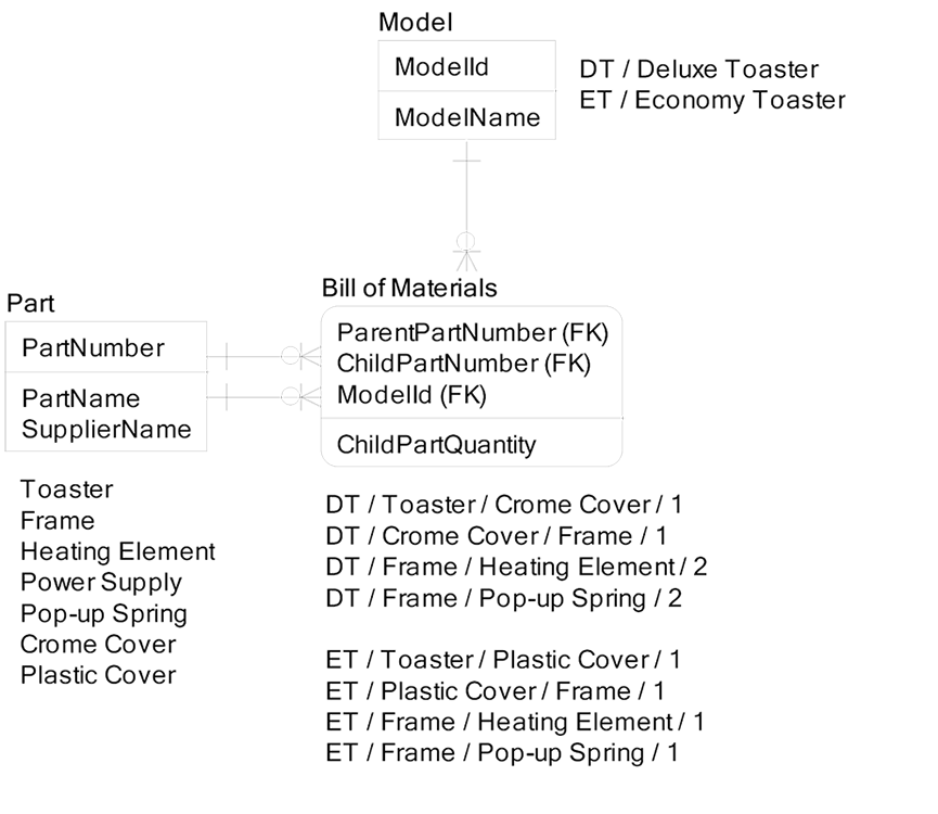
I have two models of toasters, the Deluxe Toaster and the Economy Toaster. I am forecasting next month’s needs for parts, given a forecast of next month’s sales. My sales staff assures me they will move 800 deluxe units and 1200 cheap units. I must determine how many parts we will need next month.

We first need to enter the Bill of Materials in the Model table using seed quantities of 800 Deluxe Toasters and 1200 Economy Toasters. Then we can explode from the parent parts to the child parts, and add up the child quantities along the traversal chain to determine the order quantity for each part for next month until there are no more child parts found for all pathways. Next we determine the delta between “parts on hand” and “next month’s parts requirements”, and order additional parts to fill the parts on hand deficit.

The From –> To pairs of linked nodes create networks of pathways to traverse. These pathways can have different patterns. There are both directed acyclic and directed cyclic graphs. Directed acyclic graphs contain node pairs that have a direction and always find an edge when traversing from the entry point node to all neighbors, examples include:

• Parent Animal –> Offspring Animal
• Assembly Part –> Component Part
• Component Part –> Raw Material

Directed acyclic graphs contain node pairs that have a direction and may never find an edge node due to an infinite loop of links, examples include:

• From Network Router Node -> To Network Router Node
• Friend -> Friended Friend

Luke had been curiously silent and motionless. For a talkative squirmy boy, this worried me. I asked him to summarize today’s lesson on recursion. He blurted out his frustrations and confusion, asking for me to “pleeease do the summary.” I stood my ground and insisted that Luke try a brief summary. Squirming and anxious, Luke said “I’d like to curse once now, and then I will re-curse again later. No, seriously dad, I am lost on this topic.” I granted a reprieve and summarized recursion on his behalf.

Key Points

• Recursive data models are good at describing the fact that product and service designs exist at different scales, such as starting with a “big” thing like a toaster and ending with a small component such as a spring release:
• Deluxe Toaster → Frame → Heating Element → Spring Release
• When we build a product or service from its design, we construct big finished goods from small components.

Luke and I covered one last lesson on relationship design.

Occam’s Razor for Relationship Design

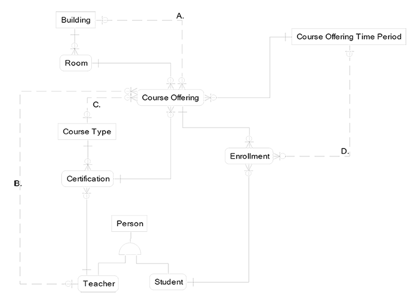
William of Occam said that when two theories are competing on a single topic, the theory with the fewest assumptions wins. While designing relationships in a data model, the model with no redundant relationships wins. Luke jumped in and requested we use a school as the example for redundant relationships that violate Occam’s rule of simplicity.

I obliged by developing the diagram on the next page, where all of the relationship lines that are dashed are redundant and should be removed. The four redundant relationships are labeled A, B, C, and D:

1. Course Offering already has the Building Id since it came from the Room to Course Offering relationship (solid line).
2. Course Offering already has Teacher Id since it came from the Certification to Course Offering relationship (solid line).
3. Course Offering already has the Course Type Id since it came from the Certification to Course Offering relationship (solid line).
4. Enrollment already has the Course Offering Time Period Id since it came from the Course Offering to Enrollment relationship (solid line).

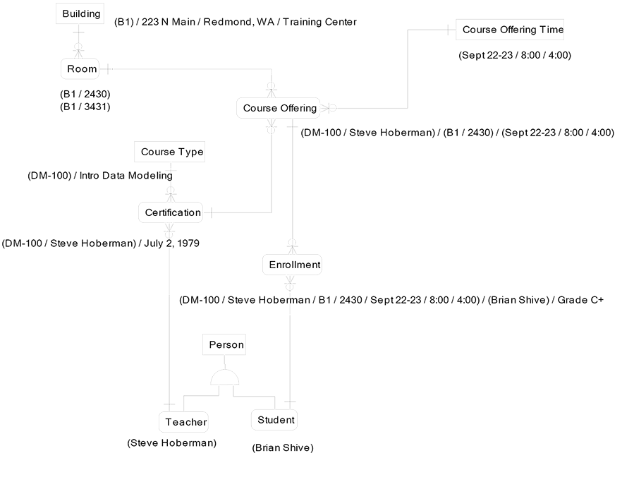
The data model on the next page is the proper model with no redundant relationships:

Classification Hierarchies

Classification hierarchies have two types of participant entities, the super-type entity and the sub-type entities under the super-type. The super-type entity is an abstraction that covers all the sub-type entities. Abstraction provides simplification of the data model and stability when the business changes requirements. The super-type entity contains the attributes that all sub-type entities have in common. The sub-type entities have attributes that are unique to themselves.

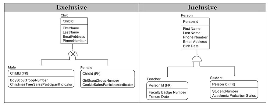
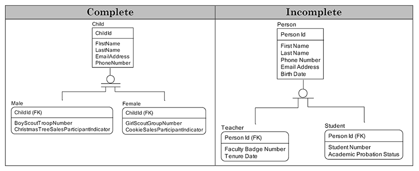
Exclusive vs. Inclusive Sub-types

In exclusive sub-types, each member of the super-type can be present in only one of the sub-types. In the following example, each child is either a male or a female. No person is both. The “x” in the symbol means exclusive sub-types. With inclusive sub-types, each member of the super-type can be one or more of the sub-types. In the following example, a person can be both a teacher for some classes and can be a student for other classes. Teachers can enroll as students. The absence of an “x” in the symbol means inclusive sub-types.

Complete vs. Incomplete Sub-types

In complete sub-types, the set of sub-types shown is the full set expected to be tracked by the business. For example, the Male and Female sub-types could be the complete set of sub-types expected to be used by a business. The complete indicator in this notation is the double lines under the circle. With incomplete sub-types, the set of sub-types is expected to be extended as the business evolves over time. For example, a school may data model just teachers and students, knowing that later there will be janitors, counselors, and other types of person tracked in their school. The single line under the sub-type symbol in this notation indicates an incomplete sub-type.

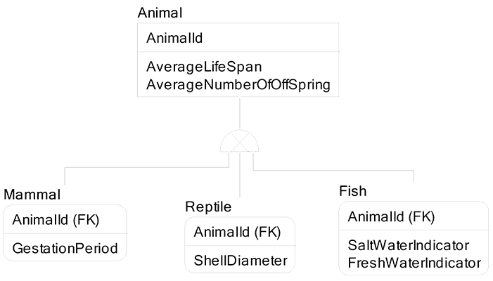
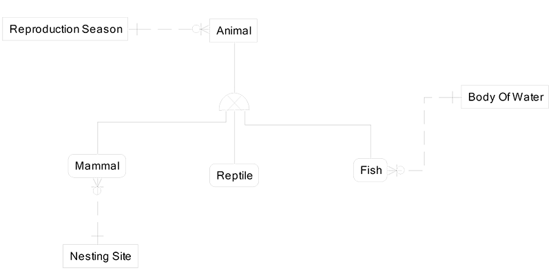
On the next page is a classification hierarchy for the entity Animal:

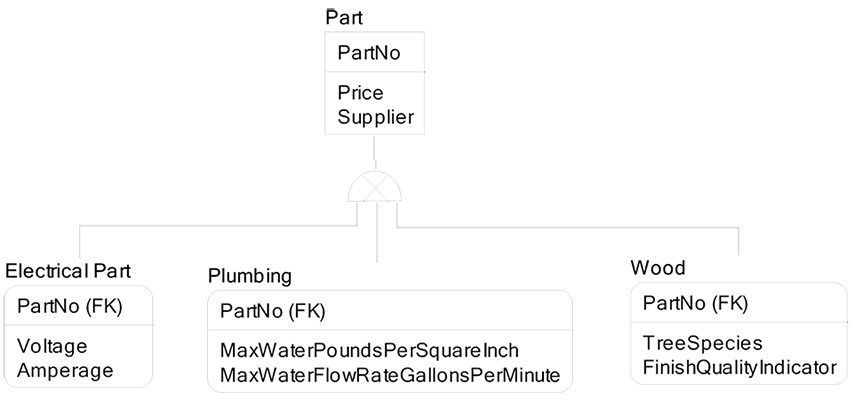
Since Luke and I had a fun visit with the house building project, I tried an example of construction parts:

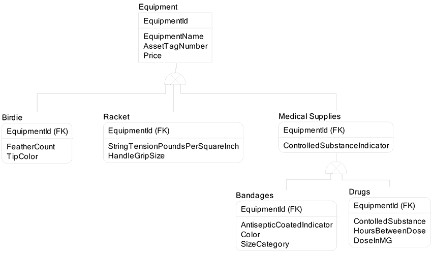
Luke wondered about the value of classification hierarchy. I explained that it is like his example of the badminton birdie having a Feather Count attribute and the racket having a String Tension attribute:

In classification hierarchies, we can specify at the CDM level which attributes belong to which entities, as we have done in the Part classification hierarchy above. Then, in the LDM and PDM, we can abstract the attributes to make them easily extensible when the business demands change. This involves an entity called Attribute and must be done carefully to avoid over abstraction. One additional value to super-types and sub-types is that we can specify relationships at either level to gain a more precise picture of the relationships being modeled.

For example, in the data model below the super-type entity Animal is related to Reproduction Season. If we did not have Animal, then we would have to relate Mammal and Reptile and Fish to Reproduction Season. Further, the Nesting Site entity is related to Mammal and not to Reptile or Fish. Finally, the Body of Water entity is related to Fish only and is not relevant to Reptile and Mammal:

One-to-One Peer to Peer Relationships

There are times when two entities are of equal importance and they have a one to one relationship. This situation is rare, but it does happen, and is frequently modeled incorrectly. Below we allow this IRS database to record information about a person who may or may not have a Social Security number:

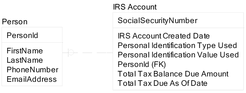
When a person gets assigned a Social Security number, a new row is inserted in the IRS Account entity that is linked to the proper Person Id.

Key Points

• The classification of the things around us into categories allows us to make behavioral generalizations, which, while not always true, will be true often enough to give us lots of value.
• One-to-one relationships between entities exist that are not classification hierarchies (peer to peer relationships above). These are surprisingly frequently missed by data modelers.

Modeling Time and Historical Events

The conceptual data model may or may not model the history of data values changing over time. Most CDMs model the current state of an entity without regard to the state of data in the past. The exceptions would be systems that have stringent requirements around tracking history. For example, banking applications are highly oriented to tracking history, so they would have historical entities in their CDM. Systems that are less attuned to history, such as instant messaging systems, will have fewer entities dedicated to historical tracking, and the CDM may ignore history completely.

The logical data model and physical data model for all systems will articulate the places where history is required to be tracked. Again, some systems have very few requirements to track history and would have few historical entities and attributes in their LDM and PDM. This is rare since most systems have several historical tracking requirements.

When modeling history, there will be two types of entities. First are “static entities” that do not change over time. Second are “dynamic entities” that do change over time

Static Entities

Static entities are the anchor points for their neighbor entities that have the purpose of tracking changes over time for some aspect of the anchor entity. For example, Person has these unchanging attributes:

• Birth date
• Birth location
• Biological mother
• Biological father

And Building has these unchanging attributes:

• Date occupancy permit granted
• City
• State

Dynamic Historical Entities

Associated to each static or anchor entity will be entities that track change over time for a particular type of change. For example, Person has these dynamic entities:

• Job History
• Marriage History
• Residence History
• Health History
• Hobby History

And Building these dynamic entities:

• Remodel History
• Cleaning History
• Handicap Access Upgrade History
• Landscape Upgrade History

In the logical data model, the history entities typically have a natural key that includes the date and time of the event being tracked. Some history entities include both the start date and time and the end date and time of the event being tracked, so the interval of the chunk of time is clearly known. Further, the granularity of time varies for each type of historical event. Fine-grain time units would be nanoseconds or milliseconds. Coarse-grain time units would be months or years. Different historical event types will have different time granularities:

• Date only for 24-hour granularity, for example Wedding Date
• Date and time to the minute, for example Contract Signed Time
• Date and time to the millisecond, for example Network Packet Delay

Below are examples of Person anchor, history entities, and date attributes:

• Employment History has Employment Start Date and Employment End Date
• Marriage History has Marriage Start Date and Marriage End Date
• Residence History has Residence Start Date and Residence End Date
• Health History has Test Date and Time, Diagnosis Date and Time, and Surgery Date and Time
• Hobby History has Hobby Start Date and Hobby End Date

And examples of Building anchor, history entities, and date attributes:

• Remodel History has Remodel Start Date and Remodel End Date
• Cleaning History has Cleaning Date
• Handicap Access Upgrade History has Handicap Access Upgrade Start Date and Time and Handicap Access Upgrade End Date and Time
• Landscape Upgrade History has Landscape Upgrade Start Date and Landscape Upgrade End Date

Standard data modeling rules for uniqueness are applied by comparing primary key values in the rows to detect duplicates. When date ranges become part of the uniqueness criteria, we must add application logic to detect intersecting date and time ranges. This logic is an extension of the traditional data value uniqueness criteria. Therefore, when we include date ranges to track history with start and end dates, we need to use application logic to maintain the uniqueness of rows.

Uniqueness that relies on application code is bad for system complexity and maintainability. But with no declarative database date range options, we must rely on programmer-developed logic to enforce most of the rules for historical databases. There are three basic types of date ranges:

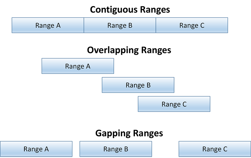
In contiguous date ranges, the end of “Range A” is one unit of time before the start of “Range B”. For example, if Marriage is tracked by minute, then my divorce must be complete one minute before my next marriage can be started (example is contiguous to the minute):

• Marriage A–End Date Time = Jan 1, 2010, 1:01 PM
• Marriage B–Start Date Time = Jan 1, 2010, 1:02 PM

In overlapping date ranges, “Range A” can end after the start of “Range B”. If Marriage allows polygamy, then my divorce for “marriage A” need not be complete before my “marriage B” can start (example shows one minute of polygamy):

• Marriage A–End Date Time = Jan 1, 2010, 1:01 PM
• Marriage B–Start Date Time = Jan 1, 2010, 1:00 PM

In gapping date ranges, the end of “Range A” can have a gap before the start of “Range B”. If Marriage allows for people to be unmarried for a period of time, which happens, then the end of one marriage can have a gap before the start of the next marriage

• Marriage A–End Date Time = Jan 1, 2010, 1:01 PM
• Marriage B–Start Date Time = Sept 26, 2012, 3:00 PM

Below is an example with data that uses a range type of contiguous for all history entities. This means that a person’s employment history can have no gaps. This is a hypothetical design, since in reality, people may have employment gaps.

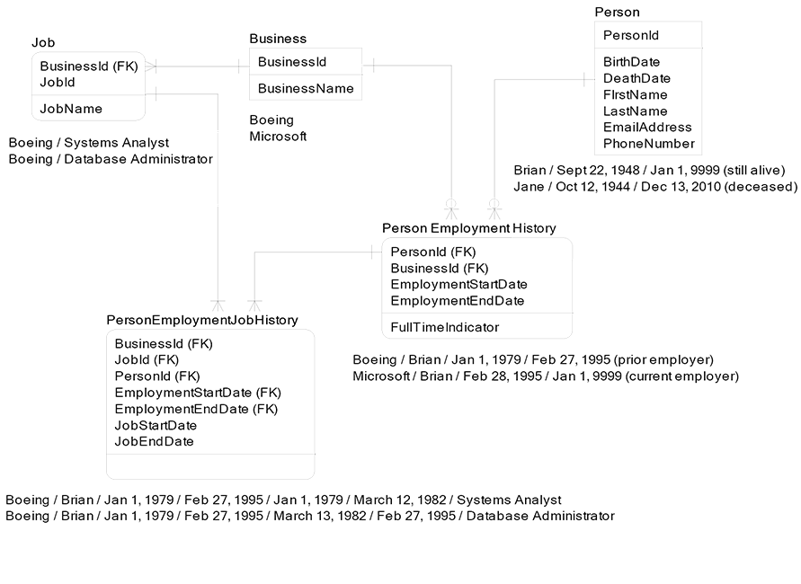
Traditional referential integrity rules between a primary key and the related foreign keys have extra logic for historical data referential integrity. Traditional referential integrity would enforce that each row in PersonEmploymentHistory already exists in Person before creating a new row in PersonEmploymentHistory. Now, when we are dealing with history tables, there is one additional referential integrity check to ensure that the PersonEmploymentHistory date ranges fall between the Person attributes of BirthDate and DeathDate.

In common sense language, we need to ensure that every person must be employed between the person’s birth date and death date. We only employ living people. Again, this self-evident rule is difficult to implement in most physical databases.

The next level of date range referential integrity rule deals with the entity PersonEmploymentJobHistory. This entity tracks the jobs that a person does when that person is employed by a business. Further, all rows in PersonEmploymentJobHistory must exist during the date ranges in PersonEmploymentHistory.

If I worked for a business called Boeing between Jan 1, 2000 and Jan 1 2010, then all my rows in PersonEmploymentJobHistory for me at Boeing must exist during the date ranges of Jan 1, 2000 and Jan 1, 2010, which is the time I was employed at Boeing. In common sense language, all job history rows for a given person in a given business must happen during that person’s employment at that business. No surprises here, but again, believe it or not, most databases do not support this obvious rule easily.

I asked Luke if he had any questions about the three types of date ranges or date range referential integrity. Luke suddenly looked confused and said, “Can’t we have date range rules that combine more than one of the three types of range rules?” Again, I was startled to find his thinking to be so perceptive. I replied, “Yes, in the real world there are history rules that use multiple range types to enforce uniqueness.”

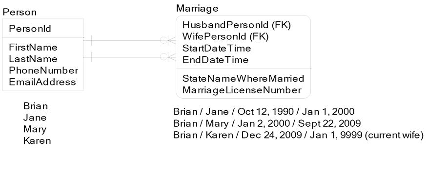
To make the point, I hopped onto my data modeling tool and pounded out this example, which uses both contiguous and gapping referential integrity history range types. Brian’s first marriage was contiguous with his second marriage. Brian’s second marriage was gapping with his third marriage:

Key Points

• The passage of time is such an integral aspect of our awareness that it is hard to imagine that most database management systems do a poor job of implementing historical data requirements. Additionally, data modeling of time is often ignored or designed inconsistently.
• We have design techniques for specification of history requirements in data models that are consistent and expressive. For implementation of history in physical databases, get ready to work hard.

Normalization

Normalization theory was originally created by mathematicians to guide database designers in how to conform to the set operation rules of the Structured Query Language (SQL) and how to avoid update anomalies. The theory eliminated redundancy of attributes, making updates easy since each fact resided in one and only one place. Each fact also had the exact unique key to give it a distinct context.

For example, the fact called Shoe Size 12D is more meaningful when you know it belongs to a given individual. Note the exception to “no redundancy” is the propagation of primary keys from one entity to another entity as a foreign key. This PK-FK redundancy is mostly managed by the referential integrity rules of database management systems.

The theory of normalization has been expressed in non-mathematical terms many times. The contents and implications of this theory vary widely between most non-mathematical presentations. These pragmatic interpretations of normalization theory present valuable insights into data modeling design principles. No single normalization interpretation is the whole truth of good data model design. I will present my own flavor of a pragmatic interpretation of normalization theory that aligns closely with Extended Relational Analysis.

Entities have attributes that identify unique instances of the entity, and other attributes that describe each instance of the entity. Any given attribute is either part of the entity’s primary key, or is a descriptive or non-primary-key attribute. Normalization theory guides us in designing which descriptive attributes belong in a given entity.

First, we must design the primary key of the entity to determine the uniqueness of rows. Second, we must design the set of descriptive Attributes that belong in the entity along with the primary key. Third, we must look for multiple uniqueness constraints beyond the primary key and document those alternate keys. Finally, we can take one last look at the non-key attributes to see if they belong in the entity considering the alternate keys.

Normalization theory will state that Attribute X is dependent on Attribute Y. The phrase “is dependent on” would be more clearly stated as “is uniquely identified by.” Normalization rules state, for example:

• Tax Amount Due is dependent on Social Security Number and Filing Year
• Person Skill Level is dependent on Hobby Identifier and Social Security Number

Which translated into clear language:

• Tax Amount Due is uniquely identified by Social Security Number and Filing Year
• Person Skill Level is uniquely identified by Hobby Identifier and Social Security Number

First Normal Form

First normal form means all attributes are atomic and not repeating. Each attribute contains atomic data. Atomic data is a collection of data that is acted on as a unit. Example, in the Person entity, the Full Name attribute should be changed to be the attributes First Name and Last Name to conform to first normal form. Searching for a first name that equals Jean Luc is hard when we store the Full Name, since there can be different people with names like:

• First Name = Jean Luc and Last Name = Ponty
• First Name = Jean and Last Name = Luc Ponty

When we tell the database about the atomic components of compound things, then the database can properly understand them. If we hide the atomic components of compound things, then developers need to guess where the boundaries were intended to exist, which is a bad choice. No attribute is repeated. For example, in the Person entity, attributes Hobby1, Hobby2, Hobby3 would be a repeating group and violate first normal form. Alternatively, the attribute Hobbies List, with a list of hobbies separated by commas, is also a violation of first normal form, as it is a repeating group, too. Hobby belongs in a new entity that is outside of the Person entity.

Second Normal Form

Second normal form means attributes can’t be dependent on a subset of the key. An entity is in second normal form when it is in first normal form and no non-primary-key attributes depend on a subset of the key. Second normal form only applies to entities with compound primary keys or with compound alternate keys. If an entity has a single attribute primary key and single attribute alternate keys, then second normal form does not apply. Example:

An entity called Person Hobby has a compound primary key consisting of Person Id and Hobby Id. If I put an attribute into Person Hobby called Last Name, I have violated second normal form, since Last Name depends on PersonId, and PersonId is only half of the primary key. Last Name is not dependent on HobbyId. The example below is a violation of second normal form:

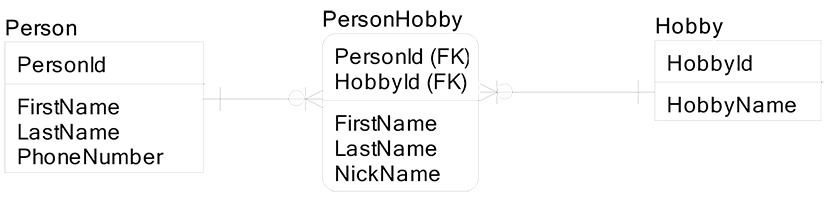
In the entity Person Hobby, the attributes First Name and Last Name are a violation of second normal form since they are uniquely identified by a subset of the PK called Person Id. Further, if someone updated their Last Name in the Person entity and forgot to update their Last Name in the Person Hobby entity, then we would have an update anomaly. When the database is in a contradictory state, different people can think I have different last names, when in reality I only have one current last name.

The attribute Nickname in the entity Person Hobby is not a violation, since I allow each person to change his or her nickname for each hobby. When I play tennis with my brother, he prefers the nickname Racketman, and when I play soccer with my brother he prefers the nickname Hot Shot.

Third Normal Form

Third normal form means attributes cannot be dependent on a superset of the key. An entity is in third normal form when it is in both first and second normal forms and no attributes of the entity are dependent on non-primary key attributes for their meaning. For example, the entity Employee below has a primary key of Employee Id. The entity also contains non-primary key attributes of Salary Type and Salary Dollar Amount. Salary Type can be either hourly or salaried. Salary Dollar Amount will contain rows with values like $15.00, $14.00, $22.00, $47,000, $57,555. Not surprisingly, when rows of data have a group in the teens and twenties and another group of values in the tens of thousands, you suspect the column is serving multiple purposes. Further, set operations on the attribute Salary Dollar Amount would be meaningless across the two salary types of hourly and salaried, especially when it is time to calculate paychecks.

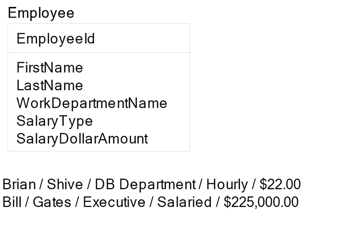
Salary Amount depends on both the Employee Id and the Salary Type. Since Salary Type is outside of the primary key, this is violation of third normal form.

To fix this example so that it conforms to third normal form requires us to add two new entities called Salaried Employee and Hourly Employee:

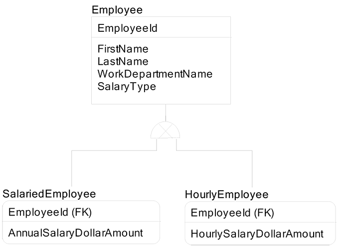
These two new entities are sub-types of the super-type entity of Employee. A one-to-one relationship exists between Employee and both Salaried Employee and Hourly Employee.

Now we can do meaningful entity-wide set operations on the attribute AnnualSalaryDollarAmount in Salaried Employee, and on the attribute HourlySalaryDollarAmount in Hourly Employee.

Normalization of Intersections

Many-to-many entities can have two or more identifying relationships in the intersection entity. This topic can be approached under normalization forms beyond the third normal form, but I prefer a simpler approach that has a common sense relationship to discovery over time and minimal relationships. This is yet another use of Occam’s Razor.

These intersection entities can also be called associative entities. The issue in normalization of intersections is to decide how many identifying relationships to put in each many-to-many entity. Intersection normalization must honor the sequence of knowing things and use as few relationships in an intersection as possible. For example, I am going to start recording my friends and the hobbies they do with me, as well as the locations where we do the hobby and the equipment used to do it. I could choose to track all these relationships in a single intersection entity that represents a four-way intersection, as diagramed on the facing page.

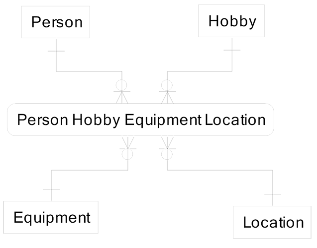
Rarely, if ever, is this correct. This design ignores the sequence of discovery of friends, hobbies, and their relationships. It also uses the maximum set of relationships in the four-way intersection entity, Person Hobby Equipment Location. No information can be recorded in the data model about relationships until we know everything.

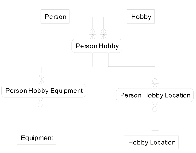
A better design is to consider that we first come to know a person plays a hobby and would like to capture this fact. Later we will ask about the equipment the person uses or where the person plays the hobby. The sequence is to first meet the person and then find out the person plays a hobby. Then we either know the equipment for the person’s hobby or the location where the person plays the hobby, as shown in the following diagram.

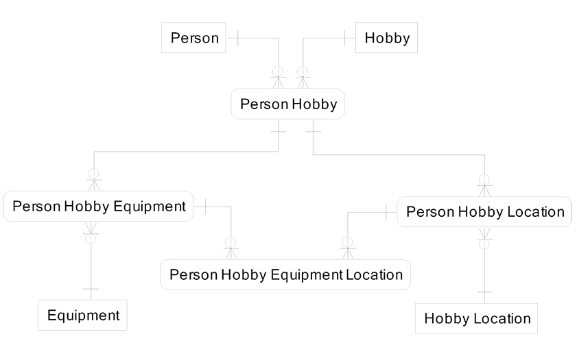
Later we discover that there may be special sports where a single hobby uses different equipment based on the location where it is being played. In this case, we must add a fact (Person Hobby Equipment Location) that is uncovered last in the sequence of fact discovery, as shown in the diagram on the next page. It will be populated rarely since most hobbies use identical equipment for all locations.

Luke was totally burned out after my diatribe on normalization, as was I. He missed at least half the ideas, but when we go to actually build his database to run his business, we would revisit these normalization concepts.

Before we launched into the final topic, we went to the beach to play in the sand and watch the waves crash into themselves. The ocean tends to clear out the mind and make space for new ideas to take root. I got sunburn while Luke, with his darker skin, played in the sun all day and showed few signs of overexposure.

Key Points

• Normalization is an important set of rules that constrain how logical data models are designed.
• Like the jazz musician, sitar player, and sports star in the zone, we have our data model rules, and yet we have an astronomic free space for creativity.
• Learn the rules, follow the rules, yet be creative. Structure and creativity are both needed for good designing.

Master Data, Transactional Data, and Measurement Data

When we returned, the final new idea for data modeling would be presented to a refreshed and ready-to-learn Luke. The final lesson was the distinction between master data, transactional data, and measurements of the world.

Master data is highly shared across processes and users. It is generally created by a small group and is viewed by a large group. Examples include: Product, Customer, Date, Sales Status, Order Status and Billing Status.

Transactional data is narrowly shared across processes and users. It is generally created by a large group, but it is viewed by a small group who are associated with the transaction. Very few processes and users can view transactional data, such as:

• Contract (I can’t see your contract)
• Order (I can’t see your order)
• Invoice (I would like to give you my invoice to pay it, but you refuse)
• Return (I would like to return your product for a refund to me, but can’t)

Measurement data is master and transactional data transformed for metrics. Measurement data is used by those needing to evaluate the success or failure of some aspect of the business, such as for Point of Sale Fact examples are Customer Dimension, Product Dimension, Time Dimension, and Store Dimension.

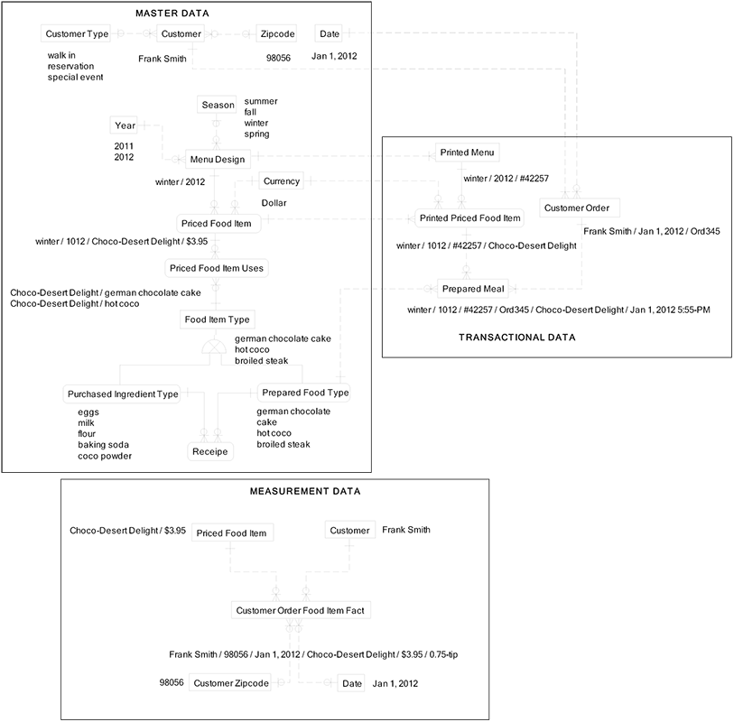
When looking at a data model, look for entities that are either master, transactional, or measurement. For example, in the following data model there are subject area boxes around the entities for master data, transactional data and measurement data.

I added sample data intended to quickly clarify the meaning of this restaurant data model. It is intended to clarify the distinctions between master data, transactional data, and measurement data:

Key Points

• Conceptual, logical, and physical data designs are best understood when the contents of the designs are categorized by master data, transactional data, and measurement data. Often, data models will mix master, transactional, and measurement data without clearly identifying these categories.
• This three-way categorization brings clarity to the semantic value of the models, as well as uniting the thinking of diverse participants in the business and IT.