
CHAPTER 18
Smoothing Methods
In this chapter, we describe a set of popular and flexible methods for forecasting time series that rely on smoothing. Smoothing is based on averaging over multiple periods in order to reduce the noise. We start with two simple smoothers, the moving average and simple exponential smoother, which are suitable for forecasting series that contain no trend or seasonality. In both cases, forecasts are averages of previous values of the series (the length of the series history considered and the weights used in the averaging differ between the methods). We also show how a moving average can be used, with a slight adaptation, for data visualization. We then proceed to describe smoothing methods suitable for forecasting series with a trend and/or seasonality. Smoothing methods are data-driven, and are able to adapt to changes in the series over time. Although highly automated, the user must specify smoothing constants that determine how fast the method adapts to new data. We discuss the choice of such constants, and their meaning. The different methods are illustrated using the Amtrak ridership series.
Python
In this chapter, we will use numpy and pandas for data handling and matplotlib for visualization. Models are built using statsmodels. We also make use of functions singleGraphLayout() and graphLayout() defined in Table 17.2. Use the following import statements to run the Python code in this chapter.
![]() import required functionality for this chapter
import required functionality for this chapter
import numpy as np
import pandas as pd
import matplotlib.pylab as plt
import statsmodels.formula.api as sm
from statsmodels.tsa import tsatools
from statsmodels.tsa.holtwinters import ExponentialSmoothing
18.1 Introduction1
A second class of methods for time series forecasting is smoothing methods. Unlike regression models, which rely on an underlying theoretical model for the components of a time series (e.g., linear trend or multiplicative seasonality), smoothing methods are data-driven, in the sense that they estimate time series components directly from the data without assuming a predetermined structure. Data-driven methods are especially useful in series where patterns change over time. Smoothing methods “smooth” out the noise in a series in an attempt to uncover the patterns. Smoothing is done by averaging the series over multiple periods, where different smoothers differ by the number of periods averaged, how the average is computed, how many times averaging is performed, and so on. We now describe two types of smoothing methods that are popular in business applications due to their simplicity and adaptability. These are the moving average method and exponential smoothing.
18.2 Moving Average
The moving average is a simple smoother: it consists of averaging values across a window of consecutive periods, thereby generating a series of averages. A moving average with window width w means averaging across each set of w consecutive values, where w is determined by the user.
In general, there are two types of moving averages: a centered moving average and a trailing moving average. Centered moving averages are powerful for visualizing trends, because the averaging operation can suppress seasonality and noise, thereby making the trend more visible. In contrast, trailing moving averages are useful for forecasting. The difference between the two is in terms of the window’s location on the time series.
Centered Moving Average for Visualization
In a centered moving average, the value of the moving average at time t (MAt) is computed by centering the window around time t and averaging across the w values within the window:
For example, with a window of width w = 5, the moving average at time point t = 3 means averaging the values of the series at time points 1, 2, 3, 4, 5; at time point t = 4, the moving average is the average of the series at time points 2, 3, 4, 5, 6, and so on.2 This is illustrated in Figure 18.1 a.

Figure 18.1 Schematic of centered moving average (a) and trailing moving average (b), both with window width w = 5
Choosing the window width in a seasonal series is straightforward: because the goal is to suppress seasonality for better visualizing the trend, the default choice should be the length of a seasonal cycle. Returning to the Amtrak ridership data, the annual seasonality indicates a choice of w = 12. Figure 18.2 (smooth blue line) shows a centered moving average line overlaid on the original series. We can see a global U-shape, but unlike the regression model that fits a strict U-shape, the moving average shows some deviation, such as the slight dip during the last year.
![]() code for creating Figure 18.2
code for creating Figure 18.2
# Load data and convert to time series
Amtrak_df = pd.read_csv('Amtrak.csv')
Amtrak_df['Date'] = pd.to_datetime(Amtrak_df.Month, format='%d/%m/%Y')
ridership_ts = pd.Series(Amtrak_df.Ridership.values, index=Amtrak_df.Date,
                         name='Ridership')
ridership_ts.index = pd.DatetimeIndex(ridership_ts.index,
                                      freq=ridership_ts.index.inferred_freq)

# centered moving average with window size = 12
ma_centered = ridership_ts.rolling(12, center=True).mean()

# trailing moving average with window size = 12
ma_trailing = ridership_ts.rolling(12).mean()

# shift the average by one time unit to get the next day predictions
ma_centered = pd.Series(ma_centered[:-1].values, index=ma_centered.index[1:])
ma_trailing = pd.Series(ma_trailing[:-1].values, index=ma_trailing.index[1:])


fig, ax = plt.subplots(figsize=(8, 7))
ax = ridership_ts.plot(ax=ax, color='black', linewidth=0.25)
ma_centered.plot(ax=ax, linewidth=2)
ma_trailing.plot(ax=ax, style='--', linewidth=2)
ax.set_xlabel('Time')
ax.set_ylabel('Ridership')
ax.legend(['Ridership', 'Centered Moving Average', 'Trailing Moving Average'])

plt.show()
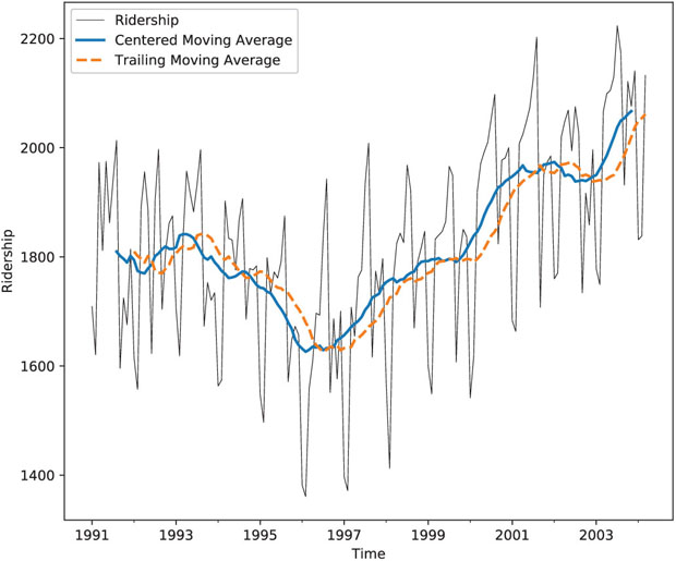
Figure 18.2 Centered moving average (smooth blue line) and trailing moving average (broken orange line) with window w = 12, overlaid on Amtrak ridership series
Trailing Moving Average for Forecasting
Centered moving averages are computed by averaging across data in the past and the future of a given time point. In that sense, they cannot be used for forecasting because at the time of forecasting, the future is typically unknown. Hence, for purposes of forecasting, we use trailing moving averages, where the window of width w is set on the most recent available w values of the series. The k-step ahead forecast Ft + k (k = 1, 2, 3, …) is then the average of these w values (see also bottom plot in Figure 18.1):
For example, in the Amtrak ridership series, to forecast ridership in February 1992 or later months, given information until January 1992 and using a moving average with window width w = 12, we would take the average ridership during the most recent 12 months (February 1991 to January 1992). Figure 18.2 (broken blue line) shows a trailing moving average line overlaid on the original series.
Next, we illustrate a 12-month moving average forecaster for the Amtrak ridership. We partition the Amtrak ridership time series, leaving the last 36 months as the validation period. Applying a moving average forecaster with window w = 12, we obtained the output shown in Figure 18.3. Note that for the first 12 records of the training period, there is no forecast (because there are less than 12 past values to average). Also, note that the forecasts for all months in the validation period are identical (1938.481) because the method assumes that information is known only until March 2001.
![]() code for creating Figure 18.3
code for creating Figure 18.3
# partition the data
nValid = 36
nTrain = len(ridership_ts) - nValid

train_ts = ridership_ts[:nTrain]
valid_ts = ridership_ts[nTrain:]

# moving average on training
ma_trailing = train_ts.rolling(12).mean()
last_ma = ma_trailing[-1]

# create forecast based on last moving average in the training period
ma_trailing_pred = pd.Series(last_ma, index=valid_ts.index)

fig, axes = plt.subplots(nrows=2, ncols=1, figsize=(9, 7.5))
ma_trailing.plot(ax=axes[0], linewidth=2, color='C1')
ma_trailing_pred.plot(ax=axes[0], linewidth=2, color='C1', linestyle='dashed')
residual = train_ts - ma_trailing
residual.plot(ax=axes[1], color='C1')
residual = valid_ts - ma_trailing_pred
residual.plot(ax=axes[1], color='C1', linestyle='dashed')
graphLayout(axes, train_ts, valid_ts)
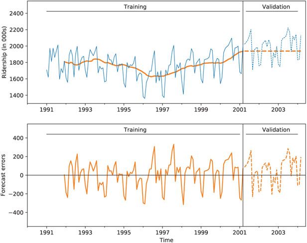
Figure 18.3 Trailing moving average forecaster with w = 12 applied to Amtrak ridership series
In this example, it is clear that the moving average forecaster is inadequate for generating monthly forecasts because it does not capture the seasonality in the data. Seasons with high ridership are under-forecasted, and seasons with low ridership are over-forecasted. A similar issue arises when forecasting a series with a trend: the moving average “lags behind,” thereby under-forecasting in the presence of an increasing trend and over-forecasting in the presence of a decreasing trend. This “lagging behind” of the trailing moving average can also be seen in Figure 18.2.
In general, the moving average should be used for forecasting only in series that lack seasonality and trend. Such a limitation might seem impractical. However, there are a few popular methods for removing trends (de-trending) and removing seasonality (de-seasonalizing) from a series, such as regression models. The moving average can then be used to forecast such de-trended and de-seasonalized series, and then the trend and seasonality can be added back to the forecast. For example, consider the regression model shown in Figure 17.6 in Chapter 17, which yields residuals devoid of seasonality and trend (see bottom chart). We can apply a moving average forecaster to that series of residuals (also called forecast errors), thereby creating a forecast for the next forecast error. For example, to forecast ridership in April 2001 (the first period in the validation set), assuming that we have information until March 2001, we use the regression model in Table 17.6 to generate a forecast for April 2001 [which yields 2004.271 thousand (=2,004,271) riders]. We then use a 12-month moving average (using the period April 2000 to March 2001) to forecast the forecast error for April 2001, which yields 30.78068 (manually, or using Python, as shown in Table 18.1). The positive value implies that the regression model’s forecast for April 2001 is too low, and therefore we should adjust it by adding approximately 31 thousand riders to the regression model’s forecast of 2004.271 thousand riders.
Table 18.1 Applying MA to the residuals from the regression model (which lack trend and seasonality), to forecast the April 2001 residual
 code for applying moving average to residuals
# Build a model with seasonality, trend, and quadratic trend
ridership_df = tsatools.add_trend(ridership_ts, trend='ct')
ridership_df['Month'] = ridership_df.index.month

# partition the data
train_df = ridership_df[:nTrain]
valid_df = ridership_df[nTrain:]

formula = 'Ridership ~ trend + np.square(trend) + C(Month)'
ridership_lm_trendseason = sm.ols(formula=formula, data=train_df).fit()

# create single-point forecast
ridership_prediction = ridership_lm_trendseason.predict(valid_df.iloc[0, :])

# apply MA to residuals
ma_trailing = ridership_lm_trendseason.resid.rolling(12).mean()

print('Prediction', ridership_prediction[0])
print('ma_trailing', ma_trailing[-1])
Output
Prediction 2004.2708927644996
ma_trailing 30.78068462405899
Choosing Window Width (w)
With moving average forecasting or visualization, the only choice that the user must make is the width of the window (w). As with other methods such as k-nearest neighbors, the choice of the smoothing parameter is a balance between under-smoothing and over-smoothing. For visualization (using a centered window), wider windows will expose more global trends, while narrow windows will reveal local trends. Hence, examining several window widths is useful for exploring trends of differing local/global nature. For forecasting (using a trailing window), the choice should incorporate domain knowledge in terms of relevance of past values and how fast the series changes. Empirical predictive evaluation can also be done by experimenting with different values of w and comparing performance. However, care should be taken not to overfit!
18.3 Simple Exponential Smoothing
A popular forecasting method in business is exponential smoothing. Its popularity derives from its flexibility, ease of automation, cheap computation, and good performance. Simple exponential smoothing is similar to forecasting with a moving average, except that instead of taking a simple average over the w most recent values, we take a weighted average of all past values, such that the weights decrease exponentially into the past. The idea is to give more weight to recent information, yet not to completely ignore older information.
Like the moving average, simple exponential smoothing should only be used for forecasting series that have no trend or seasonality. As mentioned earlier, such series can be obtained by removing trend and/or seasonality from raw series, and then applying exponential smoothing to the series of residuals (which are assumed to contain no trend or seasonality).
The exponential smoother generates a forecast at time t + 1 (Ft + 1) as follows:
where α is a constant between 0 and 1 called the smoothing parameter. The above formulation displays the exponential smoother as a weighted average of all past observations, with exponentially decaying weights.
It turns out that we can write the exponential forecaster in another way, which is very useful in practice:
where Et is the forecast error at time t. This formulation presents the exponential forecaster as an “active learner”: It looks at the previous forecast (Ft) and how far it was from the actual value (Et), and then corrects the next forecast based on that information. If in one period the forecast was too high, the next period is adjusted down. The amount of correction depends on the value of the smoothing parameter α. The formulation in (18.3) is also advantageous in terms of data storage and computation time: it means that we need to store and use only the forecast and forecast error from the most recent period, rather than the entire series. In applications where real-time forecasting is done, or many series are being forecasted in parallel and continuously, such savings are critical.
Note that forecasting further into the future yields the same forecast as a one-step-ahead forecast. Because the series is assumed to lack trend and seasonality, forecasts into the future rely only on information until the time of prediction. Hence, the k-step ahead forecast is equal to
The smoothing parameter α, which is set by the user, determines the rate of learning. A value close to 1 indicates fast learning (that is, only the most recent values have influence on forecasts) whereas a value close to 0 indicates slow learning (past values have a large influence on forecasts). This can be seen by plugging 0 or 1 into equation (18.2) or (18.3). Hence, the choice of α depends on the required amount of smoothing, and on how relevant the history is for generating forecasts. Default values that have been shown to work well are around 0.1–0.2. Some trial and error can also help in the choice of α: examine the time plot of the actual and predicted series, as well as the predictive accuracy (e.g., MAPE or RMSE of the validation set). Finding the α value that optimizes predictive accuracy on the validation set can be used to determine the degree of local vs. global nature of the trend. However, beware of choosing the “best α” for forecasting purposes, as this will most likely lead to model overfitting and low predictive accuracy on future data. To use exponential smoothing in Python, we use the ExponentialSmoothing method in statmodels. Argument smoothing_level sets the value of α. Figure 18.4 Output for simple exponential smoothing forecaster with To illustrate forecasting with simple exponential smoothing, we return to the residuals from the regression model, which are assumed to contain no trend or seasonality. To forecast the residual on April 2001, we apply exponential smoothing to the entire period until March 2001, and use α = 0.2. The forecasts of this model are shown in Figure 18.4. The forecast for the residual (the horizontal broken line) is 14.143 (in thousands of riders), implying that we should adjust the regression’s forecast by adding 14,143 riders to that forecast. In both smoothing methods, the user must specify a single parameter: In moving averages, the window width (w) must be set; in exponential smoothing, the smoothing parameter (α) must be set. In both cases, the parameter determines the importance of fresh information over older information. In fact, the two smoothers are approximately equal if the window width of the moving average is equal to w = 2/α − 1.Choosing Smoothing Parameter α
![]() code for creating Figure 18.4
code for creating Figure 18.4residuals_ts = ridership_lm_trendseason.resid
residuals_pred = valid_df.Ridership - ridership_lm_trendseason.predict(valid_df)
fig, ax = plt.subplots(figsize=(9,4))
ridership_lm_trendseason.resid.plot(ax=ax, color='black', linewidth=0.5)
residuals_pred.plot(ax=ax, color='black', linewidth=0.5)
ax.set_ylabel('Ridership')
ax.set_xlabel('Time')
ax.axhline(y=0, xmin=0, xmax=1, color='grey', linewidth=0.5)
# run exponential smoothing
# with smoothing level alpha = 0.2
expSmooth = ExponentialSmoothing(residuals_ts, freq='MS')
expSmoothFit = expSmooth.fit(smoothing_level=0.2)
expSmoothFit.fittedvalues.plot(ax=ax)
expSmoothFit.forecast(len(valid_ts)).plot(ax=ax, style='--', linewidth=2, color='C0')
singleGraphLayout(ax, [-550, 550], train_df, valid_df)

 = 0.2, applied to the series of residuals from the regression model (which lack trend and seasonality). The forecast value is 14.143
Relation Between Moving Average and Simple Exponential Smoothing
18.4 Advanced Exponential Smoothing
As mentioned earlier, both the moving average and simple exponential smoothing should only be used for forecasting series with no trend or seasonality; series that have only a level and noise. One solution for forecasting series with trend and/or seasonality is first to remove those components (e.g., via regression models). Another solution is to use a more sophisticated version of exponential smoothing, which can capture trend and/or seasonality.
Series with a Trend
For series that contain a trend, we can use “double exponential smoothing.” Unlike in regression models, the trend shape is not assumed to be global, but rather, it can change over time. In double exponential smoothing, the local trend is estimated from the data and is updated as more data arrive. Similar to simple exponential smoothing, the level of the series is also estimated from the data, and is updated as more data arrive. The k-step-ahead forecast is given by combining the level estimate at time t (Lt) and the trend estimate at time t (Tt):
Note that in the presence of a trend, one-, two-, three-step-ahead (etc.), forecasts are no longer identical. The level and trend are updated through a pair of updating equations:
The first equation means that the level at time t is a weighted average of the actual value at time t and the level in the previous period, adjusted for trend (in the presence of a trend, moving from one period to the next requires factoring in the trend). The second equation means that the trend at time t is a weighted average of the trend in the previous period and the more recent information on the change in level.3 Here there are two smoothing parameters, α and β, which determine the rate of learning. As in simple exponential smoothing, they are both constants in the range [0,1], set by the user, with higher values leading to faster learning (more weight to most recent information).
Series with a Trend and Seasonality
For series that contain both trend and seasonality, the “Holt-Winter’s Exponential Smoothing” method can be used. This is a further extension of double exponential smoothing, where the k-step-ahead forecast also takes into account the seasonality at period t + k. Assuming seasonality with M seasons (e.g., for weekly seasonality M = 7), the forecast is given by
(Note that by the time of forecasting t, the series must have included at least one full cycle of seasons in order to produce forecasts using this formula, that is, t > M.)
Being an adaptive method, Holt-Winter’s exponential smoothing allows the level, trend, and seasonality patterns to change over time. These three components are estimated and updated as more information arrives. The three updating equations are given by
The first equation is similar to that in double exponential smoothing, except that it uses the seasonally-adjusted value at time t rather than the raw value. This is done by dividing Yt by its seasonal index, as estimated in the last cycle. The second equation is identical to double exponential smoothing. The third equation means that the seasonal index is updated by taking a weighted average of the seasonal index from the previous cycle and the current trend-adjusted value. Note that this formulation describes a multiplicative seasonal relationship, where values on different seasons differ by percentage amounts. There is also an additive seasonality version of Holt-Winter’s exponential smoothing, where seasons differ by a constant amount (for more detail, see Shmueli and Lichtendahl, 2016).
![]() code for creating Figure 18.5
code for creating Figure 18.5
# run exponential smoothing with additive trend and additive seasonal
expSmooth = ExponentialSmoothing(train_ts, trend='additive', seasonal='additive',
  seasonal_periods=12, freq='MS')
expSmoothFit = expSmooth.fit()

fig, axes = plt.subplots(nrows=2, ncols=1, figsize=(9, 7.5))
expSmoothFit.fittedvalues.plot(ax=axes[0], linewidth=2, color='C1')
expSmoothFit.forecast(len(valid_ts)).plot(ax=axes[0], linewidth=2, color='C1',
                      linestyle='dashed')
residual = train_ts - expSmoothFit.fittedvalues
residual.plot(ax=axes[1], color='C1')
residual = valid_ts - expSmoothFit.forecast(len(valid_ts))
residual.plot(ax=axes[1], color='C1', linestyle='dashed')
graphLayout(axes, train_ts, valid_ts)
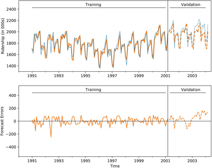
Figure 18.5 Holt-Winters exponential smoothing applied to Amtrak ridership series
To illustrate forecasting a series with the Holt-Winter’s method, consider the raw Amtrak ridership data. As we observed earlier, the data contain both a trend and monthly seasonality. Figure 18.5 depicts the fitted and forecasted values. Table 18.2 presents a summary of the model.
Table 18.2 Summary of a Holt-Winter’s exponential smoothing model applied to the Amtrak ridership data. Included are the initial and final states
> print(expSmoothFit.params)
> print('AIC: ', expSmoothFit.aic)
> print('AICc: ', expSmoothFit.aicc)
> print('BIC: ', expSmoothFit.bic)
Output
{'smoothing_level': 0.5739301428618576,
 'smoothing_slope': 4.427106197126462e-78,
 'smoothing_seasonal': 8.604237951641415e-64,
 'damping_slope': nan,
 'initial_level': 1659.4023614918137,
 'initial_slope': 0.3287888147245162,
 'initial_seasons': array([ 31.35240029, -11.35543731, 291.69040179, 291.41159861,
        324.22688177, 279.21976391, 390.31153542, 441.32947772,
        119.95805216, 244.32751369, 235.62891276, 273.93418743]),
 'use_boxcox': False,
 'lamda': None,
 'remove_bias': False}

AIC:  1021.662594988854
AICc:  1028.239518065777
BIC:  1066.6575446748127
Series with Seasonality (No Trend)
Finally, for series that contain seasonality but no trend, we can use a Holt-Winter’s exponential smoothing formulation that lacks a trend term, by deleting the trend term in the forecasting equation and updating equations.
Exponential smoothing in Python
In Python, forecasting using exponential smoothing can be done via the ExponentialSmoothing method in the statsmodels class. This can be used for simple exponential smoothing as well as advanced exponential smoothing.
Applying this method to a time series and using forecast() or predict() will yield forecasts. To include an additive or multiplicative trend and/or seasonality, use arguments trend and seasonal, such as trend=’additive’ and seasonal=’multiplicative’. The default is None. The number of seasons is specified by seasonal_periods. You can set the smoothing parameters to specific values using arguments smoothing_level (α), smoothing_slope (β), and smoothing_seasonal (γ). Leaving them unspecified will lead to optimized values (optimized=True).
Problems
-
Impact of September 11 on Air Travel in the United States. The Research and Innovative Technology Administration’s Bureau of Transportation Statistics conducted a study to evaluate the impact of the September 11, 2001 terrorist attack on US transportation. The 2006 study report and the data can be found at https://www.bts.gov/archive/publications/estimated_impacts_of_9_11_on_us_travel/index. The goal of the study was stated as follows:
The purpose of this study is to provide a greater understanding of the passenger travel behavior patterns of persons making long distance trips before and after 9/11.
The report analyzes monthly passenger movement data between January 1990 and May 2004. Data on three monthly time series are given in file Sept11Travel.csv for this period: (1) Actual airline revenue passenger miles (Air), (2) Rail passenger miles (Rail), and (3) Vehicle miles traveled (Car).
In order to assess the impact of September 11, BTS took the following approach: using data before September 11, they forecasted future data (under the assumption of no terrorist attack). Then, they compared the forecasted series with the actual data to assess the impact of the event. Our first step, therefore, is to split each of the time series into two parts: pre- and post-September 11. We now concentrate only on the earlier time series.
- Create a time plot for the pre-event AIR time series. What time series components appear from the plot?
- Figure 18.6 shows a time plot of the seasonally adjusted pre-September-11 AIR series. Which of the following smoothing methods would be adequate for forecasting this series?
- Moving average (with what window width?)
- Simple exponential smoothing
- Holt exponential smoothing
- Holt-Winter’s exponential smoothing

Figure 18.6 Seasonally adjusted pre-September-11 AIR series
-
Relation Between Moving Average and Exponential Smoothing. Assume that we apply a moving average to a series, using a very short window span. If we wanted to achieve an equivalent result using simple exponential smoothing, what value should the smoothing coefficient take?
-
Forecasting with a Moving Average. For a given time series of sales, the training set consists of 50 months. The first 5 months’ data are shown below:
Month Sales Sept 98 27 Oct 98 31 Nov 98 58 Dec 98 63 Jan 99 59 - Compute the sales forecast for January 1999 based on a moving average with w = 4.
- Compute the forecast error for the above forecast.
-
Optimizing Holt-Winter’s Exponential Smoothing. The table below shows the optimal smoothing constants from applying exponential smoothing to data, using automated model selection:
Level 1.000 Trend 0.000 Seasonality 0.246 - The value of zero that is obtained for the trend smoothing constant means that (choose one of the following):
- There is no trend.
- The trend is estimated only from the first two periods.
- The trend is updated throughout the data.
- The trend is statistically insignificant.
- What is the danger of using the optimal smoothing constant values?
- The value of zero that is obtained for the trend smoothing constant means that (choose one of the following):
-
Department Store Sales. The time plot in Figure 18.7 describes actual quarterly sales for a department store over a 6-year period (data are available in DepartmentStoreSales.csv, data courtesy of Chris Albright).
- Which of the following methods would not be suitable for forecasting this series?
- Moving average of raw series
- Moving average of deseasonalized series
- Simple exponential smoothing of the raw series
- Double exponential smoothing of the raw series
- Holt-Winter’s exponential smoothing of the raw series
- The forecaster was tasked to generate forecasts for four quarters ahead. He therefore partitioned the data such that the last four quarters were designated as the validation period. The forecaster approached the forecasting task by using multiplicative Holt-Winter’s exponential smoothing. The smoothing parameters used were α = 0.2, β = 0.15, γ = 0.05.
- Run this method on the data.
- The forecasts for the validation set are given in Table 18.3. Compute the MAPE values for the forecasts of Q21 and Q22.
Table 18.3 Forecasts for validation series using exponential smoothing
Quarter Actual Forecast Error 21 60,800 59,384.56586 1415.434145 22 64,900 61,656.49426 3243.505741 23 76,997 71,853.01442 5143.985579 24 103,337 95,074.69842 8262.301585 - The fit and residuals from the exponential smoothing are shown in Figure 18.8. Using all the information thus far, is this model suitable for forecasting Q21 and Q22?
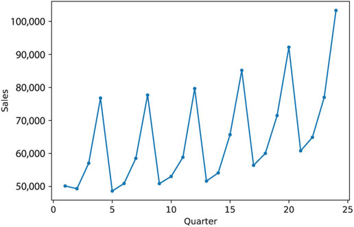
Figure 18.7 Department store quarterly sales series

Figure 18.8 Forecasts and actuals (a) and forecast errors (b) using exponential smoothing
- Which of the following methods would not be suitable for forecasting this series?
-
Shipments of Household Appliances. The time plot in Figure 18.9 shows the series of quarterly shipments (in million dollars) of US household appliances between 1985 and 1989 (data are available in ApplianceShipments.csv, data courtesy of Ken Black).
- Which of the following methods would be suitable for forecasting this series if applied to the raw data?
- Moving average
- Simple exponential smoothing
- Double exponential smoothing
- Holt-Winter’s exponential smoothing
- Apply a moving average with window span w = 4 to the data. Use all but the last year as the training set. Create a time plot of the moving average series.
- What does the MA(4) chart reveal?
- Use the MA(4) model to forecast appliance sales in Q1-1990.
- Use the MA(4) model to forecast appliance sales in Q1-1991.
- Is the forecast for Q1-1990 most likely to under-estimate, over-estimate or accurately estimate the actual sales on Q1-1990? Explain.
- Management feels most comfortable with moving averages. The analyst therefore plans to use this method for forecasting future quarters. What else should be considered before using the MA(4) to forecast future quarterly shipments of household appliances?
- We now focus on forecasting beyond 1989. In the following, continue to use all but the last year as the training set, and the last four quarters as the validation set. First, fit a regression model to sales with a linear trend and quarterly seasonality to the training data. Next, apply Holt-Winter’s exponential smoothing with smoothing parameters α = 0.2, β = 0.15, γ = 0.05 to the training data. Choose an adequate “season length.”
- Compute the MAPE for the validation data using the regression model.
- Compute the MAPE for the validation data using Holt-Winter’s exponential smoothing.
- Which model would you prefer to use for forecasting Q1-1990? Give three reasons.
- If we optimize the smoothing parameters in the Holt-Winter’s method, is it likely to get values that are close to zero? Why or why not?

Figure 18.9 Quarterly shipments of US household appliances over 5 years
- Which of the following methods would be suitable for forecasting this series if applied to the raw data?
-
Shampoo Sales. The time plot in Figure 18.10 describes monthly sales of a certain shampoo over a 3-year period. [Data are available in ShampooSales.csv, Source: Hyndman and Yang (2018).]

Figure 18.10 Monthly sales of a certain shampoo
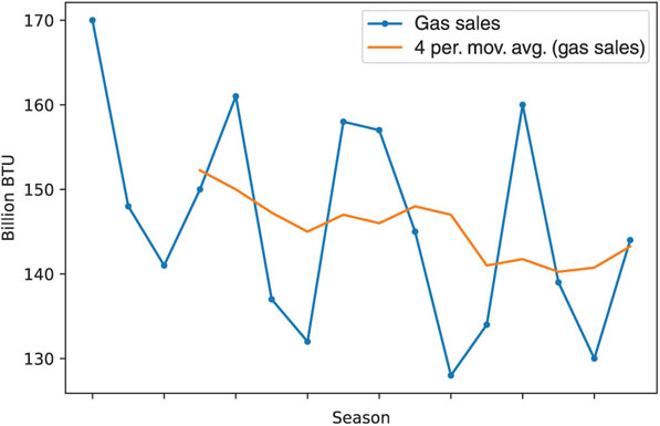
Figure 18.11 Quarterly sales of natural gas over 4 years
Which of the following methods would be suitable for forecasting this series if applied to the raw data?
- Moving average
- Simple exponential smoothing
- Double exponential smoothing
- Holt-Winter’s exponential smoothing
-
Natural Gas Sales. Figure 18.11 is a time plot of quarterly natural gas sales (in billions of BTU) of a certain company, over a period of 4 years (data courtesy of George McCabe). The company’s analyst is asked to use a moving average to forecast sales in Winter 2005.
- Reproduce the time plot with the overlaying MA(4) line.
- What can we learn about the series from the MA line?
- Run a moving average forecaster with adequate season length. Are forecasts generated by this method expected to over-forecast, under-forecast, or accurately forecast actual sales? Why?
-
Australian Wine Sales. Figure 18.12 shows time plots of monthly sales of six types of Australian wines (red, rose, sweet white, dry white, sparkling, and fortified) for 1980–1994. [Data are available in AustralianWines.csv, Source: Hyndman and Yang (2018).] The units are thousands of litres. You are hired to obtain short-term forecasts (2–3 months ahead) for each of the six series, and this task will be repeated every month.
- Which forecasting method would you choose if you had to choose the same method for all series? Why?
- Fortified wine has the largest market share of the above six types of wine. You are asked to focus on fortified wine sales alone, and produce as accurate as possible forecasts for the next 2 months.
- Start by partitioning the data using the period until December 1993 as the training set.
- Apply Holt-Winter’s exponential smoothing to sales with an appropriate season length (use smoothing parameters α = 0.2, β = 0.15, γ = 0.05).
- Create an ACF plot for the residuals from the Holt-Winter’s exponential smoothing until lag-12.
- Examining this plot, which of the following statements are reasonable conclusions?
- Decembers (month 12) are not captured well by the model.
- There is a strong correlation between sales on the same calendar month.
- The model does not capture the seasonality well.
- We should try to fit an autoregressive model with lag-12 to the residuals.
- We should first deseasonalize the data and then apply Holt-Winter’s exponential smoothing.
- How can you handle the above effect without adding another layer to your model?
- Examining this plot, which of the following statements are reasonable conclusions?

Figure 18.12 Monthly sales of six types of Australian wines between 1980 and 1994
Notes
- 1 This and subsequent sections in this chapter copyright © 2019 Datastats, LLC, and Galit Shmueli. Used by permission.
- 2 For an even window width, for example, w = 4, obtaining the moving average at time point t = 3 requires averaging across two windows: across time points 1, 2, 3, 4; across time points 2, 3, 4, 5; and finally the average of the two averages is the final moving average.
- 3 There are various ways to estimate the initial values L1 and T1, but the differences among these ways usually disappear after a few periods.