
CHAPTER 20
Text Mining
In this chapter, we introduce text as a form of data. First, we discuss a tabular representation of text data in which each column is a word, each row is a document, and each cell is a 0 or 1, indicating whether that column’s word is present in that row’s document. Then we consider how to move from unstructured documents to this structured matrix. Finally, we illustrate how to integrate this process into the standard data mining procedures covered in earlier parts of the book.
Python
In this chapter, we will use pandas for data handling and scikit-learn for the feature creation and model building. The Natural Language Toolkit will be used for more advanced text processing (nltk: https://www.nltk.org).
![]() import required functionality for this chapter
import required functionality for this chapter
from zipfile import ZipFile
import pandas as pd
from sklearn.model_selection import train_test_split
from sklearn.feature_extraction.text import CountVectorizer
from sklearn.feature_extraction.text import TfidfTransformer
from sklearn.feature_extraction.stop_words import ENGLISH_STOP_WORDS
from sklearn.decomposition import TruncatedSVD
from sklearn.preprocessing import Normalizer
from sklearn.pipeline import make_pipeline
from sklearn.linear_model import LogisticRegression
import nltk
from nltk import word_tokenize
from nltk.stem.snowball import EnglishStemmer
import matplotlib.pylab as plt
from dmba import printTermDocumentMatrix, classificationSummary, liftChart

# download data required for NLTK
nltk.download('punkt')
20.1 Introduction1
Up to this point, and in data mining in general, we have been dealing with three types of data:
- numerical
- binary (yes/no)
- multicategory
In some common predictive analytics applications, though, data come in text form. An Internet service provider, for example, might want to use an automated algorithm to classify support tickets as urgent or routine, so that the urgent ones can receive immediate human review. A law firm facing a massive discovery process (review of large numbers of documents) would benefit from a document review algorithm that could classify documents as relevant or irrelevant. In both of these cases, the predictor variables (features) are embedded as text in documents.
Text mining methods have gotten a boost from the availability of social media data—the Twitter feed, for example, as well as blogs, online forums, review sites, and news articles. According to the Rexer Analytics 2013 Data Mining Survey, between 25% and 40% of data miners responding to the survey use data mining with text from these sources. Their public availability and high profile has provided a huge repository of data on which researchers can hone text mining methods. One area of growth has been the application of text mining methods to notes and transcripts from contact centers and service centers.
20.2 The Tabular Representation of Text: Term-Document Matrix and “Bag-of-Words”
Consider the following three sentences:
S1. this is the first sentence.
S2. this is a second sentence.
S3. the third sentence is here.
We can represent the words (called terms) in these three sentences (called documents) in a term-document matrix, where each row is a word and each column is a sentence. In scikit-learn, converting a set of documents into a term-document matrix can be done by first collecting the documents into a list and then using the CountVectorizer from scikit-learn. Table 20.1 illustrates this process for the three-sentence example.
Table 20.1 Term-document matrix representation of words in sentences S1–S3
text = ['this is the first sentence.',
        'this is a second sentence.',
        'the third sentence is here.']

# learn features based on text
count_vect = CountVectorizer()
counts = count_vect.fit_transform(text)

printTermDocumentMatrix(count_vect, counts)
Output S1 S2 S3 first 1 0 0 here 0 0 1 is 1 1 1 second 0 1 0 sentence 1 1 1 the 1 0 1 third 0 0 1 this 1 1 0 |
Note that all the words in all three sentences are represented in the matrix and each word has exactly one row. Order is not important, and the number in the cell indicates the frequency of that term in that sentence. This is the bag-of-words approach, where the document is treated simply as a collection of words in which order, grammar, and syntax do not matter.
The three sentences have now been transformed into a tabular data format just like those we have seen to this point. In a simple world, this binary matrix could be used in clustering, or, with the appending of an outcome variable, for classification or prediction. However, the text mining world is not a simple one. Even confining our analysis to the bag-of-words approach, considerable thinking and preprocessing may be required. Some human review of the documents, beyond simply classifying them for training purposes, may be indispensable.
20.3 Bag-of-Words vs. Meaning Extraction at Document Level
We can distinguish between two undertakings in text mining:
- Labeling a document as belonging to a class, or clustering similar documents
- Extracting more detailed meaning from a document
The first goal requires a sizable collection of documents, or a corpus,2 the ability to extract predictor variables from documents, and for the classification task, lots of pre-labeled documents to train a model. The models that are used, though, are the standard statistical and machine learning predictive models that we have already dealt with for numerical and categorical data.
The second goal might involve a single document, and is much more ambitious. The computer must learn at least some version of the complex “algorithms” that make up human language comprehension: grammar, syntax, punctuation, etc. In other words, it must undertake the processing of a natural (i.e., noncomputer) language to understand documents in that language. Understanding the meaning of one document on its own is a far more formidable task than probabilistically assigning a class to a document based on rules derived from hundreds or thousands of similar documents.
For one thing, text comprehension requires maintenance and consideration of word order. “San Francisco beat Boston in last night’s baseball game” is very different from “Boston beat San Francisco in last night’s baseball game.”
Even identical words in the same order can carry different meanings, depending on the cultural and social context: “Hitchcock shot The Birds in Bodega Bay,” to an avid outdoors person indifferent to capitalization and unfamiliar with Alfred Hitchcock’s films, might be about bird hunting. Ambiguity resolution is a major challenge in text comprehension—does “bot” mean “bought,” or does it refer to robots?
Our focus will remain with the overall focus of the book and the easier goal—probabilistically assigning a class to a document, or clustering similar documents. The second goal—deriving understanding from a single document—is the subject of the field of natural language processing (NLP).
20.4 Preprocessing the Text
The simple example we presented had ordinary words separated by spaces, and a period to denote the end of the each sentence. A fairly simple algorithm could break the sentences up into the word matrix with a few rules about spaces and periods. It should be evident that the rules required to parse data from real-world sources will need to be more complex. It should also be evident that the preparation of data for text mining is a more involved undertaking than the preparation of numerical or categorical data for predictive models. For example, consider the modified example in Table 20.2, based on the following sentences:
Table 20.2 Term-document matrix representation of words in sentences S1–S4 (example 2)
text = ['this is the first     sentence!!',
        'this is a second Sentence :)',
        'the third sentence, is here ',
        'forth of all sentences']

# Learn features based on text. Special characters are excluded in the analysis
count_vect = CountVectorizer()
counts = count_vect.fit_transform(text)

printTermDocumentMatrix(count_vect, counts)
Output S1 S2 S3 S4 all 0 0 0 1 first 1 0 0 0 forth 0 0 0 1 here 0 0 1 0 is 1 1 1 0 of 0 0 0 1 second 0 1 0 0 sentence 1 1 1 0 sentences 0 0 0 1 the 1 0 1 0 third 0 0 1 0 this 1 1 0 0 |
S1.  this is the first     sentence!!
S2.  this is a second Sentence :)
S3.  the third sentence, is here
S4.  forth of all sentences
This set of sentences has extra spaces, non-alpha characters, incorrect capitalization, and a misspelling of “fourth.”
Tokenization
Our first simple dataset was composed entirely of words found in the dictionary. A real set of documents will have more variety—it will contain numbers, alphanumeric strings like date stamps or part numbers, web and e-mail addresses, abbreviations, slang, proper nouns, misspellings, and more.
Tokenization is the process of taking a text and, in an automated fashion, dividing it into separate “tokens” or terms. A token (term) is the basic unit of analysis. A word separated by spaces is a token. 2+3 would need to be separated into three tokens, while 23 would remain as one token. Punctuation might also stand as its own token (e.g., the @ symbol). These tokens become the row headers in the data matrix. Each text mining software program will have its own list of delimiters (spaces, commas, colons, etc.) that it uses to divide up the text into tokens. By default, the tokenizer in CountVectorizer ignores numbers and punctuation marks as shown in Table 20.2. In Table 20.3, we modify the default tokenizer to consider punctuation marks. This captures the emoji and the emphasis of the first sentence.
For a sizeable corpus, tokenization will result in a huge number of variables—the English language has over a million words, let alone the non-word terms that will be encountered in typical documents. Anything that can be done in the preprocessing stage to reduce the number of terms will aid in the analysis. The initial focus is on eliminating terms that simply add bulk and noise.
Some of the terms that result from the initial parsing of the corpus might not be useful in further analyses and can be eliminated in the preprocessing stage. For example, in a legal discovery case, one corpus of documents might be e-mails, all of which have company information and some boilerplate as part of the signature. These terms might be added to a stopword list of terms that are to be automatically eliminated in the preprocessing stage.
Table 20.3 Tokenization of S1–S4 example
text = ['this is the first     sentence!!',
        'this is a second Sentence :)',
        'the third sentence, is here ',
        'forth of all sentences']

# Learn features based on text. Include special characters that are part of a word
# in the analysis
count_vect = CountVectorizer(token_pattern='[a-zA-Z!:)]+')
counts = count_vect.fit_transform(text)

printTermDocumentMatrix(count_vect, counts)
Output S1 S2 S3 S4 :) 0 1 0 0 a 0 1 0 0 all 0 0 0 1 first 1 0 0 0 forth 0 0 0 1 here 0 0 1 0 is 1 1 1 0 of 0 0 0 1 second 0 1 0 0 sentence 0 1 1 0 sentence!! 1 0 0 0 sentences 0 0 0 1 the 1 0 1 0 third 0 0 1 0 this 1 1 0 0 |
Text Reduction
Most text-processing software (the CountVectorizer class in scitkit-learn included) come with a generic stopword list of frequently occurring terms to be removed. If you review scikit-learn’s stopword list during preprocessing stages, you will see that it contains a large number of terms to be removed (Table 20.4 shows the first 180 stopwords). You can provide your own list of stopwords using the stop_words keyword argument to CountVectorizer.
Additional techniques to reduce the volume of text (“vocabulary reduction”) and to focus on the most meaningful text include:
- Stemming, a linguistic method that reduces different variants of words to a common core.
- Frequency filters can be used to eliminate either terms that occur in a great majority of documents or very rare terms. Frequency filters can also be used to limit the vocabulary to the n most frequent terms.
- Synonyms or synonymous phrases may be consolidated.
- Letter case (uppercase/lowercase) can be ignored.
- A variety of specific terms in a category can be replaced with the category name. This is called normalization. For example, different e-mail addresses or different numbers might all be replaced with “emailtoken” or “numbertoken.”
Table 20.5 presents the text reduction step applied to the four sentences example, after tokenization. We can see the number of terms has been reduced to five.
Presence/Absence vs. Frequency
The bag-of-words approach can be implemented either in terms of frequency of terms, or presence/absence of terms. The latter might be appropriate in some circumstances—in a forensic accounting classification model, for example, the presence or absence of a particular vendor name might be a key predictor variable, without regard to how often it appears in a given document. Frequency can be important in other circumstances, however. For example, in processing support tickets, a single mention of “IP address” might be non-meaningful—all support tickets might involve a user’s IP address as part of the submission. Repetition of the phrase multiple times, however, might provide useful information that IP address is part of the problem (e.g., DNS resolution). Note: The CountVectorizer by default returns the frequency option. To implement the presence/absence option, you need to use the argument binary=True so that the vectorizer returns a binary matrix (i.e., convert all non-zero counts to 1’s).
Table 20.4 Stopwords in scikit-learn
from sklearn.feature_extraction.stop_words import ENGLISH_STOP_WORDS
stopWords = list(sorted(ENGLISH_STOP_WORDS))
ncolumns = 6; nrows= 30

print('First {} of {} stopwords'.format(ncolumns * nrows, len(stopWords)))
for i in range(0, len(stopWords[:(ncolumns * nrows)]), ncolumns):
    print(”.join(word.ljust(13) for word in stopWords[i:(i+ncolumns)]))
First 180 of 318 stopwords a about above across after afterwards again against all almost alone along already also although always am among amongst amoungst amount an and another any anyhow anyone anything anyway anywhere are around as at back be became because become becomes becoming been before beforehand behind being below beside besides between beyond bill both bottom but by call can cannot cant co con could couldnt cry de describe detail do done down due during each eg eight either eleven else elsewhere empty enough etc even ever every everyone everything everywhere except few fifteen fifty fill find fire first five for former formerly forty found four from front full further get give go had has hasnt have he hence her here hereafter hereby herein hereupon hers herself him himself his how however hundred i ie if in inc indeed interest into is it its itself keep last latter latterly least less ltd made many may me meanwhile might mill mine more moreover most mostly move much must my myself name namely neither never nevertheless next nine no nobody none noone nor not |
Term Frequency–Inverse Document Frequency (TF-IDF)
There are additional popular options that factor in both the frequency of a term in a document and the frequency of documents with that term. One such popular option, which measures the importance of a term to a document, is Term Frequency–Inverse Document Frequency (TF-IDF). For a given document d and term t, the term frequency (TF) is the number of times term t appears in document d:
Table 20.5 Text Reduction of S1–S4 (after tokenization)
text = ['this is the first     sentence!! ',
        'this is a second Sentence :)',
        'the third sentence, is here ',
        'forth of all sentences']

# Create a custom tokenizer that will use NLTK for tokenizing and lemmatizing
# (removes interpunctuation and stop words)
class LemmaTokenizer(object):
    def __init__(self):
        self.stemmer = EnglishStemmer()
        self.stopWords = set(ENGLISH_STOP_WORDS)

    def __call__(self, doc):
        return [self.stemmer.stem(t) for t in word_tokenize(doc)
                if t.isalpha() and t not in self.stopWords]

# Learn features based on text
count_vect = CountVectorizer(tokenizer=LemmaTokenizer())
counts = count_vect.fit_transform(text)

printTermDocumentMatrix(count_vect, counts)
Output S1 S2 S3 S4 forth 0 0 0 1 second 0 1 0 0 sentenc 1 1 1 1 |
TF(t, d) = # times term t appears in document d.
To account for terms that appear frequently in the domain of interest, we compute the Inverse Document Frequency (IDF) of term t, calculated over the entire corpus and defined as3
The addition of 1 makes sure that terms for which the logarithm is zero are not ignored in the analysis
TF-IDF(t, d) for a specific term–document pair is the product of TF(t, d) and IDF(t):
The TF-IDF matrix contains the value for each term-document combination. The above definition of TF-IDF is a common one, however, there are multiple ways to define and weight both TF and IDF, so there are a variety of possible definitions of TF-IDF. For example, Table 20.6 shows the TF-IDF matrix for the four-sentence example (after tokenization and text reduction). The function TfidfTransformer class uses the natural logarithm for the computation of IDF. For example, the TF-IDF value for the term “first” in document 1 is computed by
The general idea of TF-IDF is that it identifies documents with frequent occurrences of rare terms. TF-IDF yields high values for documents with a relatively high frequency for terms that are relatively rare overall, and near-zero values for terms that are absent from a document, or present in most documents.
Table 20.6 TF-IDF Matrix for S1–S4 example (after tokenization and text reduction)
text = ['this is the first     sentence!!',
        'this is a second Sentence :)',
        'the third sentence, is here ',
        'forth of all sentences']

# Apply CountVectorizer and TfidfTransformer sequentially
count_vect = CountVectorizer()
tfidfTransformer = TfidfTransformer(smooth_idf=False, norm=None)
counts = count_vect.fit_transform(text)
tfidf = tfidfTransformer.fit_transform(counts)

printTermDocumentMatrix(count_vect, tfidf)
Output S1 S2 S3 S4 all 0.000000 0.000000 0.000000 2.386294 first 2.386294 0.000000 0.000000 0.000000 forth 0.000000 0.000000 0.000000 2.386294 here 0.000000 0.000000 2.386294 0.000000 is 1.287682 1.287682 1.287682 0.000000 of 0.000000 0.000000 0.000000 2.386294 second 0.000000 2.386294 0.000000 0.000000 sentence 1.287682 1.287682 1.287682 0.000000 sentences 0.000000 0.000000 0.000000 2.386294 the 1.693147 0.000000 1.693147 0.000000 third 0.000000 0.000000 2.386294 0.000000 this 1.693147 1.693147 0.000000 0.000000 |
From Terms to Concepts: Latent Semantic Indexing
In Chapter 4, we showed how numerous numeric variables can be reduced to a small number of “principal components” that explain most of the variation in a set of variables. The principal components are linear combinations of the original (typically correlated) variables, and a subset of them serve as new variables to replace the numerous original variables.
An analogous dimension reduction method—latent semantic indexing [or latent semantic analysis, (LSA)]—can be applied to text data. The mathematics of the algorithm are beyond the scope of this chapter,4 but a good intuitive explanation comes from the user guide for XLMiner software5:
For example, if we inspected our document collection, we might find that each time the term “alternator” appeared in an automobile document, the document also included the terms “battery” and “headlights.” Or each time the term “brake” appeared in an automobile document, the terms “pads” and “squeaky” also appeared. However, there is no detectable pattern regarding the use of the terms “alternator” and “brake” together. Documents including “alternator” might or might not include “brake” and documents including “brake” might or might not include “alternator.” Our four terms, battery, headlights, pads, and squeaky describe two different automobile repair issues: failing brakes and a bad alternator.
So, in this case, latent semantic indexing would reduce the four terms to two concepts:
- brake failure
- alternator failure
We illustrate latent semantic indexing using Python in the example in Section 20.6.
Extracting Meaning
In the simple latent semantic indexing example, the concepts to which the terms map (failing brakes, bad alternator) are clear and understandable. In many cases, unfortunately, this will not be true—the concepts to which the terms map will not be obvious. In such cases, latent semantic indexing will greatly enhance the manageability of the text for purposes of building predictive models, and sharpen predictive power by reducing noise, but it will turn the model into a blackbox device for prediction, not so useful for understanding the roles that terms and concepts play. This is OK for our purposes—as noted earlier, we are focusing on text mining to classify or cluster new documents, not to extract meaning.
20.5 Implementing Data Mining Methods
After the text has gone through the preprocessing stage, it is then in a numeric matrix format and you can apply the various data mining methods discussed earlier in this book. Clustering methods can be used to identify clusters of documents—for example, large numbers of medical reports can be mined to identify clusters of symptoms. Prediction methods can be used with tech support tickets to predict how long it will take to resolve an issue. Perhaps the most popular application of text mining is for classification—also termed labeling—of documents.
20.6 Example: Online Discussions on Autos and Electronics
This example6 illustrates a classification task—to classify Internet discussion posts as either auto-related or electronics-related. One post looks like this:
From: [email protected] (Tom Smith) Subject: Ford Explorer 4WD - do I need performance axle?
We’re considering getting a Ford Explorer XLT with 4WD and we have the following questions (All we would do is go skiing - no off-roading):
1. With 4WD, do we need the “performance axle” - (limited slip axle). Its purpose is to allow the tires to act independently when the tires are on different terrain.
2. Do we need the all-terrain tires (P235/75X15) or will the all-season (P225/70X15) be good enough for us at Lake Tahoe?
Thanks,
Tom
–
================================================
Tom Smith Silicon Graphics [email protected] 2011 N. Shoreline Rd. MS 8U-815 415-962-0494 (fax) Mountain View, CA 94043
================================================
The posts are taken from Internet groups devoted to autos and electronics, so are pre-labeled. This one, clearly, is auto-related. A related organizational scenario might involve messages received by a medical office that must be classified as medical or non-medical (the messages in such a real scenario would probably have to be labeled by humans as part of the preprocessing).
The posts are in the form a zipped file that contains two folders: auto posts and electronics posts, each contains a set of 1000 posts organized in small files. In the following, we describe the main steps from preprocessing to building a classification model on the data. Table 20.7 provides Python code for the text processing step for this example. We describe each step separately next.
Importing and Labeling the Records
The ZipFile module in the standard library of Python is used to read the individual documents in the zipped datafile. We additionally create a label array that corresponds to the order of the documents—we will use “1” for autos and “0” for electronics. The assignment is based on the file path (see Step 1 in Table 20.7).
Table 20.7 Importing and Labeling the records, preprocessing text, and producing concept matrix
# Step 1: import and label records
corpus = []
label = []
with ZipFile('AutoAndElectronics.zip') as rawData:
    for info in rawData.infolist():
        if info.is_dir():
            continue
        label.append(1 if 'rec.autos' in info.filename else 0)
        corpus.append(rawData.read(info))

# Step 2: preprocessing (tokenization, stemming, and stopwords)
class LemmaTokenizer(object):
    def __init__(self):
        self.stemmer = EnglishStemmer()
        self.stopWords = set(ENGLISH_STOP_WORDS)
    def __call__(self, doc):
        return [self.stemmer.stem(t) for t in word_tokenize(doc)
                if t.isalpha() and t not in self.stopWords]

preprocessor = CountVectorizer(tokenizer=LemmaTokenizer(), encoding='latin1')
preprocessedText = preprocessor.fit_transform(corpus)

# Step 3: TF-IDF and latent semantic analysis
tfidfTransformer = TfidfTransformer()
tfidf = tfidfTransformer.fit_transform(preprocessedText)

# Extract 20 concepts using LSA ()
svd = TruncatedSVD(20)
normalizer = Normalizer(copy=False)
lsa = make_pipeline(svd, normalizer)

lsa_tfidf = lsa.fit_transform(tfidf) |
Text Preprocessing in Python
The text preprocessing step does tokenization into words followed by stemming and removal of stopwords. These two operations are shown in Step 2 in Table 20.7.
Producing a Concept Matrix
The preprocessing step will produce a “clean” corpus and term-document matrix that can be used to compute the TF-IDF term-document matrix described earlier. The TF-IDF matrix incorporates both the frequency of a term and the frequency with which documents containing that term appear in the overall corpus. We use here the default settings for the TfidfTransformer.
The resulting matrix is probably too large to efficiently analyze in a predictive model (specifically, the number of predictors in the example is 13,466, so we use latent semantic indexing to extract a reduced space, termed “concepts.” For manageability, we will limit the number of concepts to 20. In scikit-learn, latent semantic indexing can be implemented by TruncatedSVD followed by normalization using Normalizer. Table 20.7 shows the Python code for applying these two operations—creating a TF-IDF matrix and latent semantic indexing—to the example.
Finally, we can use this reduced set of concepts to facilitate the building of a predictive model. We will not attempt to interpret the concepts for meaning.
Fitting a Predictive Model
At this point, we have transformed the original text data into a familiar form needed for predictive modeling—a single target variable (1 = autos, 0 = electronics), and 20 predictor variables (the concepts).
We can now partition the data (60% training, 40% validation), and try applying several classification models. Table 20.8 shows the performance of a logistic regression, with “class” as the outcome variable and the 20 concept variables as the predictors.
The confusion matrix (Table 20.8) shows reasonably high accuracy in separating the two classes of documents—an accuracy of 0.96. The decile-wise lift chart (Figure 20.1) confirms the high separability of the classes and the usefulness of this model for a ranking goal. For a two class dataset with a nearly 50/50 split between the classes, the maximum lift per decile is 2, and the lift shown here is just under 2 for the first 50% of the cases, and close to 0 for the last 40%.
Next, we would also try other models to see how they compare; this is left as an exercise.
Table 20.8 Fitting a Predictive Model to the Autos and Electronics Discussion Data
# split dataset into 60% training and 40% test set
Xtrain, Xtest, ytrain, ytest = train_test_split(lsa_tfidf, label, test_size=0.4,
                                                random_state=42)

# run logistic regression model on training
logit_reg = LogisticRegression(solver='lbfgs')
logit_reg.fit(Xtrain, ytrain)

# print confusion matrix and accuracty
classificationSummary(ytest, logit_reg.predict(Xtest))
Output Confusion Matrix (Accuracy 0.9563)
Prediction
Actual 0 1
0 389 8
1 27 376 |
Prediction
The most prevalent application of text mining is classification (“labeling”), but it can also be used for prediction of numerical values. For example, maintenance or support tickets could be used to predict length or cost of repair. The only step that would be different in the above process is the label that is applied after the preprocessing, which would be a numeric value rather than a class.
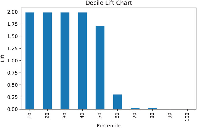
Figure 20.1 Decile-wise lift chart for autos-electronics document classification
20.7 Summary
In this chapter, we drew a distinction between text processing for the purpose of extracting meaning from a single document (natural language processing—NLP) and classifying or labeling numerous documents in probabilistic fashion (text mining). We concentrated on the latter, and examined the preprocessing steps that need to occur before text can be mined. Those steps are more varied and involved than those involved in preparing numerical data. The ultimate goal is to produce a matrix in which rows are terms and columns are documents. The nature of language is such that the number of terms is excessive for effective model-building, so the preprocessing steps include vocabulary reduction. A final major reduction takes place if we use, instead of the terms, a limited set of concepts that represents most of the variation in the documents, in the same way that principal components capture most of the variation in numerical data. Finally, we end up with a quantitative matrix in which the cells represent the frequency or presence of terms and the columns represent documents. To this we append document labels (classes), and then we are ready to use this matrix for classifying documents using classification methods.
Problems
-
Tokenization. Consider the following text version of a post to an online learning forum in a statistics course:
Thanks John!<br /><br /><font size=”3”> "Illustrations and demos will be provided for students to work through on their own"</font>. Do we need that to finish project? If yes, where to find the illustration and demos? Thanks for your help.<img title=”smile” alt=”smile” src=”url{http://lms.statistics. com/pix/smartpix.php/statistics_com_1/s/smil ey.gif}” ><br /> <br />- Identify 10 non-word tokens in the passage.
- Suppose this passage constitutes a document to be classified, but you are not certain of the business goal of the classification task. Identify material (at least 20% of the terms) that, in your judgment, could be discarded fairly safely without knowing that goal.
- Suppose the classification task is to predict whether this post requires the attention of the instructor, or whether a teaching assistant might suffice. Identify the 20% of the terms that you think might be most helpful in that task.
- What aspect of the passage is most problematic from the standpoint of simply using a bag-of-words approach, as opposed to an approach in which meaning is extracted?
-
Classifying Internet Discussion Posts. In this problem, you will use the data and scenario described in this chapter’s example, in which the task is to develop a model to classify documents as either auto-related or electronics-related.
- Load the zipped file into Python and create a label vector.
- Following the example in this chapter, preprocess the documents. Explain what would be different if you did not perform the “stemming” step.
- Use the LSA to create 10 concepts. Explain what is different about the concept matrix, as opposed to the TF-IDF matrix.
- Using this matrix, fit a predictive model (different from the model presented in the chapter illustration) to classify documents as autos or electronics. Compare its performance to that of the model presented in the chapter illustration.
-
Classifying Classified Ads Submitted Online. Consider the case of a website that caters to the needs of a specific farming community, and carries classified ads intended for that community. Anyone, including robots, can post an ad via a web interface, and the site owners have problems with ads that are fraudulent, spam, or simply not relevant to the community. They have provided a file with 4143 ads, each ad in a row, and each ad labeled as either − 1 (not relevant) or 1 (relevant). The goal is to develop a predictive model that can classify ads automatically.
- Open the file farm-ads.csv, and briefly review some of the relevant and non-relevant ads to get a flavor for their contents.
- Following the example in the chapter, preprocess the data in Python, and create a term-document matrix, and a concept matrix. Limit the number of concepts to 20.
- Examine the term-document matrix.
- Is it sparse or dense?
- Find two non-zero entries and briefly interpret their meaning, in words (you do not need to derive their calculation).
- Briefly explain the difference between the term-document matrix and the concept-document matrix. Relate the latter to what you learned in the principal components chapter (Chapter 4).
- Using logistic regression, partition the data (60% training, 40% validation), and develop a model to classify the documents as “relevant” or “non-relevant.” Comment on its efficacy.
- Why use the concept-document matrix, and not the term-document matrix, to provide the predictor variables?
-
Clustering Auto Posts. In this problem, you will use the data and scenario described in this chapter’s example. The task is to cluster the auto posts.
- Following the example in this chapter, preprocess the documents, except do not create a label vector.
- Use the LSA to create 10 concepts.
- Before doing the clustering, state how many natural clusters you expect to find.
- Perform hierarchical clustering and inspect the dendrogram.
- From the dendrogram, how many natural clusters appear?
- Examining the dendrogram as it branches beyond the number of main clusters, select a sub-cluster and assess its characteristics.
- Perform k-means clustering for two clusters and report how distant and separated they are (using between-cluster distance and within cluster dispersion).
Notes
- 1 This and subsequent sections in this chapter copyright © 2019 Datastats, LLC, and Galit Shmueli. Used by permission.
- 2 The term “corpus” is often used to refer to a large, fixed standard set of documents that can be used by text preprocessing algorithms, often to train algorithms for a specific type of text, or to compare the results of different algorithms. A specific text mining setting may rely on algorithms trained on a corpus specially suited to that task. One early general-purpose standard corpus was the Brown corpus of 500 English language documents of varying types (named Brown because it was compiled at Brown University in the early 1960s).
- 3 IDF(t) is actually just the fraction, without the logarithm, although using a logarithm is very common.
- 4 Generally, in PCA, the dimension is reduced by replacing the covariance matrix by a smaller one; in LSA, dimension is reduced by replacing the term-document matrix by a smaller one.
- 5 Analytic Solver Platform, XLMiner Platform, Data Mining User Guide, 2014, Frontline Systems, p. 245.
- 6 The dataset is taken from www.cs.cmu.edu/afs/cs/project/theo-20/www/data/news20.html, with minor modifications.