
Chapter 8. Building applications with TensorFlow.js
In the previous chapters, we discussed the various JavaScript concepts and frameworks that enable us to perform deep learning in the browser. In this chapter, we put all that knowledge to use and build simple, but real, applications that demonstrate the potential of the technology.
Note: All of the source code used in this book can be found here: https://github.com/backstopmedia/deep-learning-browser. And, you can access the demo of our Rock Paper Scissors game here: https://reiinakano.github.io/tfjs-rock-paper-scissors/. Also, you can access the demo of our text generation model here: https://reiinakano.github.io/tfjs-lstm-text-generation/.
Each section in this chapter represents a full stand-alone web application written in TensorFlow.js, starting with a link to a live online demo you can visit to play around with the application. We then go into the details of the underlying deep learning algorithms used in the project. After this, a full explanation of the program flow is given, complete with a line-by-line discussion of the TensorFlow.js components.
Our hope is that you will be able to use these small projects as a guideline, serving as a minimal reference for you to apply your own models and business logic to build out a deep learning-based application of your own.
Gesture classification using TensorFlow.js
In this section, we’ll use TensorFlow.js to play Rock Paper Scissors with our webcam! Before trying to explain what exactly that means, we’ve hosted the application on Github Pages so it’s easier to see for yourself how it works.
If you’ve played around with Google’s Teachable Machine, which we mentioned in an earlier chapter, you’ll notice that the training mechanics are exactly the same. To teach your browser how to recognize “Rock,” point your “Rock” gesture (probably a closed fist) at the camera, then hold down the “Train Rock” button to have your browser get snapshots. The underlying machine learning model then learns to detect when you are making the “Rock” gesture while playing the game. For robustness, make sure to have your model see different angles and positions of the “Rock” gesture. Otherwise, simply shifting your hand a few inches could make the browser think you’re doing an entirely different pose. Note that you don’t need to use hand gestures to distinguish between Rock, Paper, and Scissors. You could show it an actual rock, paper, or a pair of scissors instead!
Even when you’re not training, the browser continuously scans your webcam and classifies it as either rock, paper, or scissors. The small size of the underlying machine learning model allows us to perform both training and classification in real-time. Once you’ve trained your model on all three hand gestures, you’re ready to start playing Rock-Paper-Scissors with your browser!
The algorithm
To understand the code, it’s important to know the details of the underlying algorithm used to make the predictions.
One of the algorithm’s important characteristics is its small size and fast inference. If the browser needed to download 100MB worth of neural network weights, all your users would complain. On the other hand, if it takes ten seconds to predict a gesture, that would hardly be real-time! Fortunately, the underlying neural network model we’re using satisfies both of these requirements. SqueezeNet is a neural network architecture designed to be as small as possible while achieving acceptable accuracy for image classification. According to the original paper, SqueezeNet requires only 0.5MB of space while achieving AlexNet-level accuracy on ImageNet, which is more than enough for our application. This makes it ideal for use in environments with limited memory and processing power, such as smartphones or the browser.
We’re not, however, relying on SqueezeNet alone. Another important characteristic of our application is its ability to learn from a small amount of data. It takes only around 50 images per gesture to get reasonable performance from our model. ImageNet, on the other hand, contains millions of images, with each category containing several hundred images. How does our model perform so well with such a small amount of training data compared to ImageNet? The answer is an interesting technique called transfer learning.
The general idea behind transfer learning is to have a model learn how to solve problem, and have it use the knowledge it gains to solve a different but related problem.
The general procedure for transfer learning is simple. First, you train your neural network on a large amount of data you have available. This data should be as similar to your actual data as possible, such as images for image processing tasks. For image processing tasks, this large database is usually ImageNet. After you’ve trained your model, you “cut out” the last few layers of the network (usually just one or two) and run your own images through what’s remaining. In other words, instead of classifying your own images according to ImageNet’s categories, you get the an intermediate layer’s output for each image. The idea is that these outputs are the “features” of your own images as seen through an ImageNet-trained network. The network deconstructs the input into what it thinks are the relevant features of images in general. The closer our own images are to the ImageNet images, the better the generated features will be.
After this, we can use the extracted features to train a different classifier, presumably on our own classes. One common way to do this is to simply attach a small fully-connected neural network to our feature extractor, and do the usual training process, except this time, we freeze the parameters of the original neural network, and only update the weights of the attached network.
Transfer learning has shown remarkable results in fields where collecting domain-specific data can be very expensive, such as medical image processing.
In our application, instead of attaching a small neural network at the end of an ImageNet-trained SqueezeNet, we use the extracted features to train a K-Nearest Neighbors classifier. A K-Nearest Neighbors classifier is a machine learning model that classifies an unseen data sample by looking at the classes of the training samples that are closest to it (its neighbors). This calculation can easily be done via matrix multiplication, which is a single operation in TensorFlow.js. Since training a KNN classifier is much faster than training a neural network (all you need to do is append the training sample to a matrix), in addition to being able to learn from small amounts of data, our model can also be trained in real-time in the browser.
As a quick summary, our model is as follows:
- Using a SqueezeNet trained on ImageNet, we use the second to the last layer as a feature extractor for our webcam images.
- We use the extracted features as input to a K-Nearest Neighbors classifier, and train it on our three classes: Rock, Paper, and Scissors.
- To do inference on an image, we run it through SqueezeNet, and input the extracted features into our newly trained KNN classifier to detect our gesture. Simple!
Setting up your TensorFlow.js project
To set up all our project’s dependencies, we’ll use Yarn. For people who’ve never used Yarn, it’s a widely used dependency manager for Javascript. Although the basics are pretty intuitive, it’s worth having a look at their documentation if you want to understand how it’s used.
The main file defining the dependencies of our application is the package.json file found in the root repository. Here we define some metadata about the project, such as its name, version, and license. One particularly important part is the dependencies field, which lists down the dependencies our project uses so we can easily import them from any of our .js files. Here you’ll notice two important dependencies our project relies on: deeplearn 0.5.0 and deeplearn-knn-image-classifier 0.3.0. While deeplearn contains TensorFlow.js, deeplearn-knn-image-classifier contains all the code for the model we discussed in the previous section, wrapped up in a single easy-to-use NPM package.
To add a package, simply run yarn add <package-name> from the repository root. This command should automatically download the package and its dependencies, and update both package.json and the yarn.lock file in the repository.
Our package.json file also contains a few useful scripts for developing our application. The first important script is prep, which can be invoked from the root of the repository by calling yarn prep. This script should be run the first time you clone the repository as it makes Yarn download all dependencies needed by the project and also creates the dist folder that will contain the files created by the build process. Another important script is invoked through yarn start. This starts a development server at localhost:9966 that watches for changes in your source code and automatically refreshes your application. This allows for a very efficient development cycle. Finally, yarn build and yarn deploy use browserify and uglify-js to compile your various .js files into a single minified and production-ready .js file, for when you’re ready to deploy your application for the world to see.
Instantiating the KNN Image Classifier
We’re ready to begin examining our application’s source code. As this is a book about deep learning in the browser, we’ll only be focusing on those parts of the application. But don’t worry, the non-deep learning related code was made as simple as possible using vanilla JavaScript. No external frameworks like Vue.js or React were used. And if you are planning to use these frameworks in your own apps, it shouldn’t be at all difficult to see how you would fit them in with the TensorFlow.js code.
Let’s take a look at the KNNImageClassifier class that comes with the deeplearn-knn-image-classifier package. This class is responsible for creating the neural network, downloading pre-trained model weights, adjusting the KNN model per training image, and performing inference on new images.
Inside the main.js file at our project’s root directory, we define a Main class that is instantiated as soon as the browser window loads. The Main class’s constructor contains all the code to initialize our application’s variables. At the end of the constructor function, we see the following lines:
// Instantiate the knn modelthis.knn=newKNNImageClassifier(NUM_CLASSES,TOPK);// Load knn modelthis.knn.load().then(()=>this.start());
The first line creates the KNNImageClassifier object and assigns it to this.knn. The constructor for KNNImageClassifier takes two arguments, numClasses and k. numClasses defines how many distinct classes our model is expected to classify. In our case, this is three (one for each gesture). k is a parameter used by our model’s underlying KNN algorithm. It defines how many “neighbors” the model looks at to determine a sample’s class.
The next line calls the KNNImageClassifier instance’s load function. This function is responsible for downloading the weights for our model’s pre-trained SqueezeNet. You will notice from our use of then that the load function is actually an asynchronous function that returns a Promise. This Promise resolves when the SqueezeNet’s weights have finished downloading. When it does, we are ready to start our TensorFlow.js processing loop, which is done by calling this.start().
The TensorFlow.js processing loop
The Main.start() function is shown below.
start(){this.video.play();this.timer=requestAnimationFrame(()=>this.animate());}
It does two things: Start the webcam stream with this.video.play(), and call the first iteration of the TensorFlow.js processing loop with this.animate(). You might notice that we wrap the this.animate() call with a requestAnimationFrame. requestAnimationFrame is an asynchronous function that calls the function passed to it when the browser’s view is ready to . This ensures that we sync the browser viewport refresh rate with our processing loop. You will also notice the following line at the end of this.animate():
this.timer=requestAnimationFrame(()=>this.animate());
So at the end of a single iteration of this.animate(), we wait for the browser to refresh its viewport, then call the next iteration of our processing loop. This is a common pattern to ensure the browser gets to render properly before we line up more operations for the GPU to handle. Without this, the browser will hang up, rendering your web page unusable.
You will also notice that we assign the return value of requestAnimationFrame to a variable this.timer. Although we don’t use it in this application, this gives us the option to stop/pause our processing loop based on some event. A stop function that pauses our processing loop would look something like this:
stop(){this.video.pause();cancelAnimationFrame(this.timer);}
Let us now examine what we do in one iteration of our processing loop. Inside our animate() function, we start off with the line:
constimage=dl.fromPixels(this.video);
fromPixels is a function that converts a browser image into a 3-D Tensor containing its pixel intensities. The function captures an image from ImageData, an HTMLImageElement, an HTMLCanvasElement, or an HTMLVideoElement. In our case, we pass in the HTMLVideoElement associated with our webcam. The fromPixel function then converts the current image our webcam is showing into a Tensor3D we can use with our other TF.js functions.
Further down, we see the following lines:
// Train class if one of the buttons is held downif(this.training!=-1){// Add current image to classifierthis.knn.addImage(image,this.training);}
This snippet of code checks if we’re currently training one of our three gestures (if a train button is pressed down) and adds the image to our KNN model. This is done easily using the KNNImageClassifier instance’s addImage function. This function takes the 3D Tensor containing the new training image, and its corresponding class. Internally, the KNNImageClassifier runs the image through its pre-trained SqueezeNet, takes the resulting features extracted, and appends it to the KNN’s array of training samples.
The next block of code in our processing loop looks like this:
constexampleCount=this.knn.getClassExampleCount();if(Math.max(...exampleCount)>0){this.knn.predictClass(image).then((res)=>{// Do something with our model's prediction `res`}).then(()=>image.dispose());}else{image.dispose();}
We call this.knn.getClassExampleCount() to get the number of images per class that our model has been trained on. Then, if our model has been trained on at least one image, we go ahead and use our model to predict the class of that image.
To predict an image, pass in our Tensor3D object to the predictClass function of our KNN Image Classifier. The predictClass function is an asynchronous function, performing inference on the provided image and returning a Promise that resolves with the results of the inference. The .then attached to our predictClass call let’s us define a function to run once the inference is finished. In our case, we use the results of the inference to update the corresponding variables, text and images in the UI. Since the .then call also returns another Promise when the passed in function finishes, we can chain it with another .then call. This time, we call the dispose() method on the image Tensor3D object. This frees up the GPU memory associated with this particular Tensor. If we didn’t do this, we’d have a memory leak and run out of space as our processing loop would continuously allocate image Tensor objects per iteration.
Finally, notice that if we have yet to train our model on a single class, we’ll skip inference altogether and throw away our image Tensor using image.dispose().
To summarize, our TensorFlow.js processing loop works as follows:
- Capture an image from the camera and convert it to a
Tensor3Dusingtf.fromPixels. - Check if we are currently in the process of training a gesture. If so, add the image and corresponding label to our model using
KNNImageClassifier.addImage. - Check if our model has been trained on at least a single image. If so, perform inference on the current image being processed using
KNNImageClassifier.predictClass. Update class variables and UI elements based on the result. - Dispose the image using the
.dispose()method ofTensorobjects. - Using
requestAnimationFrame, callthis.animate()to run the next iteration of the processing loop.requestAnimationFrameensures we give the browser time to redraw its viewport before we repeat the loop. - Repeat step 1.
We have two functions left we have yet to discuss: startGame and resolveGame. These two functions contain the actual code used to run the Rock Paper Scissors game with the browser. They handle the flow of a game and watch the internal variables set by our TensorFlow.js processing loop to check which gesture the user is currently making at the camera to update the UI accordingly. However, we won’t go into the detail of these two functions as we don’t actually call any TensorFlow.js code in them. Understanding them is left as an exercise to the reader.
Wrap-up
In this section, we used the KNNImageClassifier model so we can play Rock Paper Scissors with our webcam. Since we’ve discussed the necessary parts of the TensorFlow.js processing loop used to quickly train a model from your webcam images, you can easily repurpose the code to use this functionality in your own applications.
Text Generation using TensorFlow.js
One important feature of TensorFlow.js is its ability to run models that were written and trained in Python using Keras or TensorFlow. In this section, we’ll show just how easy it is to convert a Keras model for use in TensorFlow.js.
You can explore the demo of our text generation model running on TensorFlow.js here.
The algorithm
To start off, choose one model from the numerous examples in the official Keras repository. While most of these models can be converted, we want to select one with a relatively small size. This has two advantages: the browser needs to download fewer weights, and a smaller neural network can generate predictions quicker. This increases responsiveness for the user and improves their overall experience on your web page.
We end up selecting the LSTM Text Generation model from the Keras examples repository. The model is a very simple LSTM trained on a corpus of Nietzsche texts. With a network size not bigger than half a megabyte, this model fits our criteria.
During training, the model is given 40-character segments of the text and trained to predict the next character.
To generate a sample, input an initial 40 character segment of text (the “seed”) into our model and let it try to predict the next character. We then generate a new 40 character segment by removing the first character of the seed and appending our newly predicted character at the end. We input this new 40 character text segment to get the next character. We do this as many times as we want until we get a fully generated sentence of our desired length (coherent or not).
The Keras model
Our neural network is a very simple single-layer LSTM with 128 units. The output of this layer is then connected to a single fully-connected layer with N outputs, where N is the total number of unique characters in our entire text corpus. The model can be constructed in Keras with four very concise lines:
model=Sequential()model.add(LSTM(128,input_shape=(maxlen,len(chars))))model.add(Dense(len(chars)))model.add(Activation('softmax'))
As long as we have Keras installed, we can use the given script as is, with a single modification to save the weights after training. Inside the on_epoch_end function, which is called by Keras at the end of every epoch, add this line:
defon_epoch_end(epoch,logs):model.save('lstm.h5'%epoch)...
This line saves the trained model (at the end of each epoch) as a .h5 file that we can directly convert into a TensorFlow.js Model.
Converting a Keras model into a TensorFlow.js model
TensorFlow.js makes it very easy to convert a Keras model into a TensorFlow.js Model object. The details can be found in the official documentation, but we’ll run through them quickly in this section.
After running our modified lstm_text_generation.py file, we’ll end up with a file called lstm.h5 in our working directory. This file contains our Keras model graph and the corresponding weights of the model at the latest epoch that our script has run. It contains all the information needed to recreate the model in TensorFlow.js.
TensorFlow.js provides a tool called tensorflowjs_converter that you can use to convert the Keras .h5 file. To install it, run pip install tensorflowjs on the command line. After installing, convert our model from a terminal using the following command:
$tensorflowjs_converter --input_format keraspath/to/my_model.h5 path/to/tfjs_target_dir
Replace path/to/my_model.h5 with the path to your Keras .h5 file and path/to/tfjs_target_dir to a directory that you can access from the browser.
After running the command, observe the contents of tfjs_target_dir. For our small LSTM model, we find the following files:
$ ls path/to/tfjs_target_dir
group1-shard1of1  group2-shard1of1  model.json
If you look into the files, you will see that model.json contains a full graph of the layers that compose our LSTM model, and the location of the saved weights per layer. group1-shard1of1 and group2-shard1of1 contain the saved weights of our model. Together, the files in tfjs_target_dir contain all of the information required for TensorFlow.js to exactly recreate our Keras model in the browser.
Setting up our project
We’ll use almost the same setup that we used in our previous Rock-Paper-Scissors application to set up this one. The only difference is that we don’t need to import deeplearn-knn-image-classifier.
Just as a quick recap, to start our project from scratch, run yarn prep. To start a development server for quick prototyping, run yarn start and visit localhost:9966. To add a package, run yarn add <package-name>. Finally, to compile your code into a production-ready bundle, run yarn build and yarn deploy in succession.
Importing a Keras model in TensorFlow.js
It is very easy to import our converted Keras model into a TensorFlow.js Model. All that is needed is a single call to tf.loadModel. From our application, we see the following code snippet:
tf.loadModel('lstm/model.json').then((model)=>{this.model=model;this.enableGeneration();});
tf.loadModel is an asynchronous function that loads the model from the model.json file and weights generated by the tensorflowjs_converter conversion step. The Promise returned by this function resolves with the newly created TensorFlow.js Model instance. Like any other Model object, we can use its predict method to generate predictions for some data samples. In our case, we save the returned Model into variable this.model for later access. We also call the this.enableGeneration method to set up the UI letting the user know we can start generating predictions with our model.
Note that the path we pass in to tf.loadModel is a relative path. This works just like an argument to an XML HTTP Request (XHR), meaning that TensorFlow.js will try to fetch model.json from mydomain.com/lstm/model.json. You can also pass in an absolute path to tf.loadModel. This is a common scenario in case you want to serve the model weights from a different location than your application, such as Google Cloud Storage and Amazon S3.
The TensorFlow.js processing loop
Unlike our previous application, we don’t need TensorFlow.js to be continuously running. We only need to generate predictions from our model when our user does some action, such as clicking the “Generate new text” button. We define a single asynchronous function generateText that starts a processing loop every time the user clicks this button. First, notice that during initialization, we have the following code:
this.generateButton.onclick=()=>{this.generateText();}
This ensures that every time generateButton is clicked, we start the asynchronous processing loop to generate text predictions.
Our asynchronous processing loop starts with a few UI changes:
asyncgenerateText(){this.generatedSentence.innerText=this.inputSeed.value;this.generateButton.disabled=true;...}
We copy the text from the user’s input into the element displaying the model’s generated text. This is because we consider the user’s input as the beginning of our generated text, and use it as the basis for the rest of the generated characters. We also disable the generateButton element since we don’t want the user to be able to start another processing loop while the current one is still running.
We then see the actual loop as follows:
for(leti=0;i<CHARS_TO_GENERATE;i++){constindexTensor=tf.tidy(()=>{constinput=this.convert(this.generatedSentence.innerText);constprediction=this.model.predict(input).squeeze();returnthis.sample(prediction);})constindex=awaitindexTensor.data();indexTensor.dispose();this.generatedSentence.innerText+=indices_char[index];awaittf.nextFrame();}
CHARS_TO_GENERATE dictates how many characters we want our network to generate. Since our model predicts the next characters one-by-one, we need to run our processing loop a total of CHARS_TO_GENERATE times.
The first step of our processing loop is a tf.tidy call. As discussed previously, this call helps us manage GPU memory by keeping track of all Tensors created inside the closure and releasing their memory after the function ends, except for the returned Tensor. In this case, the tf.tidy function is responsible for returning indexTensor, which is a Tensor that contains the index of the next character our model generates. It is worth pointing out at this point that since our neural network can’t directly generate characters, we create a mapping from a numeric index to a unique character of our corpus. These mappings are contained in the imported indices_char (index to unique character) and char_indices (unique character to index) variables and used whenever we want to convert some text into a model input or convert the model output into text.
We’ll examine the contents of the tf.tidy call later in more detail. For now, we move on to the next line, where we extract the data from our indexTensor using indexTensor.data(). This method triggers an asynchronous function that waits for the GPU to finish calculating indexTensor and transfers the underlying Tensor data to the CPU for our use. Since generateText is an asynchronous function, we can simply use the await keyword to wait for the indexTensor.data() call to resolve. We assign the value containing the generated character’s index to index.
After extracting the data from indexTensor, we call indexTensor.dispose() to free up any GPU resources taken by indexTensor.
Using indices_char to map index to its corresponding character, we append it to generatedSentence for displaying to the user. Finally, await tf.nextFrame() serves the same purpose that requestAnimationFrame did in our previous application. We need to wait for the browser to be ready to refresh itself before beginning the next iteration of our processing loop. This will make it so the character we just generated has a chance to display itself on the browser. Without this call, the browser would simply freeze for however long the entire processing loop takes, then display all the generated text at once, making for a terrible user experience.
Constructing the model input
Let’s examine the contents of the tf.tidy call we made earlier. As mentioned, the goal of the operations inside the tf.tidy call is to have the network predict the next character of a given text. The first step to doing this is converting our input into a Tensor object that can be processed by our Model. Do this via the following line:
constinput=this.convert(this.generatedSentence.innerText);
this.generatedSentence.innerText contains all of the generated text so far. At the very beginning of our processing loop, it will contain the user’s seed text. Every newly generated character is appended to this variable and used in the next iteration as new input to the model. The first few lines of the convert function is shown below:
convert(sentence){sentence=sentence.toLowerCase();sentence=sentence.split('').filter(x=>xinchar_indices).join('');if(sentence.length<INPUT_LENGTH){sentence=sentence.padStart(INPUT_LENGTH);}elseif(sentence.length>INPUT_LENGTH){sentence=sentence.substring(sentence.length-INPUT_LENGTH);}...}
Starting off with a JavaScript string, we do some simple preprocessing on the text, such as converting it to lower case, and removing characters that aren’t originally in the text corpus.
One important thing to remember is that our model was trained to do prediction on INPUT_LENGTH character blocks of text (in our case, INPUT_LENGTH is 40). If the sentence variable is longer than that, we cut off characters from the front of the text. If the sentence variable is shorter, pad the left side of the input with spaces.
After preprocessing, we create the Tensor representation of our 40-character block of input text. Our Tensor representation will have a shape of [1, INPUT_LENGTH, num_unique_chars]. The first dimension refers to our batch dimension. Since our original Keras model was trained using batches, the model needs a batch input. Since we only have one input per iteration, we keep the batch dimension at 1. We then focus our attention on INPUT_LENGTH and num_unique_chars. Each character in our text is represented by one row, and each row has num_unique_chars columns, where each column represents a unique character in our original text corpus. For each row, the column corresponding to its unique character is marked 1, and the rest are kept at 0.
As a quick example of this, here’s an example of our tensor if we were representing the word “cat” from an original text corpus of only 4 letters.
| a | b | c | t | |
|---|---|---|---|---|
c| 0 | 0 | 1 | 0 | | a| 1 | 0 | 0 | 0 | | t| 0 | 0 | 0 | 1 | |
This type of encoding is commonly known as one hot encoding, and is a commonly used form of encoding in machine learning, particularly in text processing.
The following code performs the one hot encoding of our text into a Tensor.
constbuffer=tf.buffer([1,INPUT_LENGTH,Object.keys(indices_char).length]);for(leti=0;i<INPUT_LENGTH;i++){letchar=sentence.charAt(i)buffer.set(1,0,i,char_indices[char]);}constinput=buffer.toTensor();returninput;
Since normal Tensor objects are immutable, we are faced with a problem when we want to set the values of a Tensor one-by-one during initialization. To solve this problem, TensorFlow.js gives us tf.TensorBuffer. A tf.TensorBuffer allows us to set its values one-by-one with a .set() method, after which we can convert it to a real Tensorobject with a single .toTensor() call.
We first create a tf.TensorBuffer with the desired shape using tf.buffer. After populating its fields with the one hot encoding of each character in our input text, we convert it to an actual Tensor object using buffer.toTensor() and return this value to the caller.
Performing a prediction
The next step in our tf.tidy call is to run our newly formed input through our LSTM model. Using the Model API, this can be done with a single line:
constprediction=this.model.predict(input).squeeze();
Our model’s output Tensor shape is [num_batches, num_unique_chars]. For each possible unique character, our LSTM generates the probability of a particular unique character being next in the sequence. Here’s an example output of our LSTM model for a batch size of 1.
| a | b | c | t |
|---|---|---|---|
0.1 | 0.2 | 0.4 | 0.3 |
In that example, our model thinks that “c” has a 40% chance of being the next character in our text, while “a” has only a 10% chance.
You may notice the .squeeze() call on our model’s output. Since we only have a batch size of 1, we can remove the redundant outer dimension from the output, leaving us with a Tensor of shape [num_unique_chars].
Sampling our model output
After getting the output of our model, the final step is to actually select the next character. As previously discussed, our model’s output gives us the probability that a particular unique character will be the next one for a given input text. The simplest way to select the next character would then be to choose the one with the highest probability. However, one side effect of this is that our model doesn’t get to “explore” around the space of possible characters. To understand this, imagine that our model takes as input the text “ca” and the following LSTM output:
| a | b | c | t |
|---|---|---|---|
0 | 0.399 | 0.2 | 0.401 |
Following the simplest strategy, we would select “t” as the next character, forming the word “cat”. However, selecting “b” would form the word “cab,” which also forms a valid word. “c” could also be a possible next character, perhaps forming “cactus” or “cache”. Looking closer at the probabilities, “b,” “t,” and “c” are fairly close in value to each other. If we always just chose the character with the highest probability, we’d always get “cat” instead of the other possibilities. If we instead sampled the characters randomly, weighted by their respective probabilities, our model would get the chance to “experiment” with different output characters, and perhaps give us more diversity in our generated text.
The sample function we call on the output does this sampling for us.
The first lines of the sample function adjusts our model’s prediction based on a certain DIVERSITY constant.
sample(prediction){returntf.tidy(()=>{prediction=prediction.log();constdiversity=tf.scalar(DIVERSITY);prediction=prediction.div(diversity);prediction=prediction.exp();adjustedPred=prediction.div(prediction.sum());...});}
To understand what these lines of code do, we’ll show a few examples of what it does for a given input and varying levels of DIVERSITY.
With prediction being a 1-D Tensor of
[0.25, 0.1, 0.2, 0.45]
and DIVERSITY at 1.0, adjustedPred becomes:
[0.25, 0.1, 0.2, 0.45].
For DIVERSITY = 10, adjustedPred is:
[0.2531058, 0.2309448, 0.2475205, 0.268429].
On the other extreme, for DIVERSITY = 0.1, adjustedPred becomes:
[0.0027921, 3e-7, 0.0002998, 0.9969078].
It’s now fairly easy to understand what’s going on. For a DIVERSITY of 1, there is no change in the model’s output. As the DIVERSITY goes up, adjustedPred’s probabilities get more evenly distributed. As it goes down, the Tensor element with the highest probability gains even more of an edge over the other elements. With this method, we can choose how much we want our model to “explore” the different characters. Set DIVERSITY too high, and we’ll basically be picking at random. Set it too low, and we’re back to our strategy of picking the character with the highest probability.
After adjusting our output predictions for the level of diversity we want, we can randomly sample from the probabilities using the following lines:
adjustedPred=adjustedPred.mul(tf.randomUniform(adjustedPred.shape));returnadjustedPred.argMax();
We multiply each element of adjustedPred with a random value sampled between 0 and 1. This way, even if a character has a lower probability, it still has a slight chance of “winning” over characters with higher probabilities. We then use the .argMax() call to select the character with the highest probability, after the multiplication with tf.randomUniform.
Wrap-up
In this section, we successfully ported an LSTM trained in Keras to TensorFlow.js. To summarize, here are the steps we took to achieve this:
- Build, train, and save our model using Keras.
- Convert the Keras generated .h5 file to a TensorFlow.js supported format using the tfjs-converter tool.
- Load the model using
tf.loadModel. - Convert input into the model’s expected
Tensorformat. - Use
Model.predict(input)to generate an output from our model. - Perform any post-processing needed on the model’s output. In this case, we sampled the model’s output to get the next character for the generated text.
Denoising images using TensorFlow.js
In this next application, we’ll build a neural network that can remove noise from handwritten digits and run it on TensorFlow.js. This will allow us to explore some of TensorFlow.js’s built-in support for image processing tasks. As in the previous application, we’ll build this demo by creating our model in Keras and porting it to TensorFlow.js using the tensorflowjs_converter tool.
You can explore a demo of the application live here.
The algorithm
The neural network architecture we’ll be using for this application is the autoencoder, or more specifically, a variation of it called a denoising autoencoder.
Simply put, an autoencoder is a neural network trained to reconstruct the input at its output. This may not make sense at first. What is the value of a neural network that simply copies its input? The main motivation behind autoencoders is compression. Shown below are the layers of a very simple autoencoder.
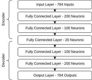
Notice how the layers progressively become smaller until it reaches the middle layer, after which the layers grow back to the original size of the input. If we are able to train this neural network to reconstruct various inputs, then we will have effectively built a compression algorithm. Our input of 784 features is represented by a middle layer of only 28 features, from which we learn to reconstruct the original image. The first half of our autoencoder is the encoder, responsible for shrinking down, or encoding, our original input from 784 features to just 28. The second half of our autoencoder is the decoder, which learns to decode the original image from the encoded representation.
Note that it is important that the training inputs be of a similar nature (e.g. audio, images) so the autoencoder can find patterns and redundancies it can compress in the data. For example, an autoencoder trained on handwritten digits might learn that 7’s are sometimes written with a dash through the middle. It may choose to represent the length of this dash as one of the features in our encoded representation. In reality though, the meaning of each of the 28 features in our encoded representation is unknown to us. The network learns the relevant features of the input on its own by seeing a large amount of data with backpropagation.
A denoising autoencoder is a variation of the autoencoder trained to remove noise from input data. The idea is simple; since an autoencoder learns to represent redundancies and patterns of a particular set of data, it will remove noise from the encoded representation of the data, after which decoding should give us the original image without noise. To train a denoising autoencoder, we give it an input sample mixed with noise, and use the original input without noise as the expected output.
In this demo, we use a denoising autoencoder built in Keras and trained on the MNIST database of handwritten digits.
Converting a Keras model into a TensorFlow.js model
You can view the source of our Keras denoising autoencoder here. Although we won’t go into detail about the Keras code, the layers used in the denoising autoencoder can be seen in the following image.
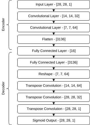
As can be seen, the original image of 28x28 has been reduced into a latent vector of only 16 features. Presumably, after training, these 16 features contain only information relevant to reconstructing a handwritten digit, and not information about noise.
As in the previous application, we need to modify the script to save a .h5 file containing the trained model to disk. Somewhere after the call to autoencoder.fit(...), add the line autoencoder.save("path/to/my_model.h5") and run the script to train and save the denoising autoencoder.
After this step, you can use the tensorflowjs_converter tool to convert the .h5 file into a TensorFlow.js compatible format.
$tensorflowjs_converter --input_format keraspath/to/my_model.h5 path/to/tfjs_target_dir
One thing you may have noticed in the Keras script is that we divide our data into training and test data. We want to make sure our denoising autoencoder also works well on digits it has never seen before. In fact, in our demo, every time “Load New Digit” is clicked, the application fetches a new image from a set of test digits not used in training the autoencoder.
Setting up our project
As we don’t need external dependencies other than tfjs, you can simply keep the package.json file we used in the previous LSTM text generation application.
Initialization
As always, the constructor method in the Main class of our application contains setup code for the various UI elements.
In this case, we set up three canvas HTML elements, which will serve as the container for the original image, the image with noise, and the image restored by the autoencoder.
After this, we set the onclick callbacks of the buttons “Load new digit” and “Reapply noise” to the updateInputTensor() and updateNoiseTensor() methods, respectively.
Finally, we load the model using the following code:
tf.loadModel('model/model.json').then((model)=>{this.model=model;this.enableGeneration();});
As before, we register an arrow function that is executed after our Model successfully loads. In the arrow function, we store the model in an instance variable this.model for later use. We also call a method this.initializeTensors() to set up some initial Tensor objects using our newly-loaded Model. We’ll go into more detail about the initializeTensors() method later.
The application flow
Our application gives the user two buttons to perform actions: “Load new digit” and “Reapply noise.”
Clicking “Load new digit” loads a new random digit from the server, adds noise to it, and runs the distorted image through the model.
On the other hand, “Reapply noise” generates new random noise, adds it to the already-loaded digit, and again runs the distorted image through the model.
Note how we always immediately run the new distorted digit through our autoencoder. This is acceptable since our model is quite small and can generate predictions very quickly. For bigger and slower models, you may consider a different application flow, such as having another button you can use to initiate a model.predict() call.
Our application flow suggests that we are keeping track of four main Tensor objects, which are the input image Tensor, the noise Tensor, the distorted image Tensor, and the denoised image Tensor. These Tensors are stored in the following instance variables: this.inputTensor, this.noiseTensor, this.distortedTensor, and this.fixedTensor. The relationship between them can be seen in the following chart:
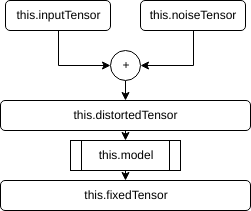
You can see that a change in inputTensor or noiseTensor will “trickle down” and change both distortedTensor and fixedTensor. In our application, we have four methods taking responsibility for updating each of these Tensor objects, namely: updateInputTensor(), updateNoiseTensor(), updateDistortedTensor(), and updateFixedTensor(). The interaction between these methods dictates our application’s entire flow.
Loading a test digit
Let’s explore the updateInputTensor() method in more detail.
updateInputTensor(){letrandInt=Math.floor(Math.random()*1002);lettemp=newImage();temp.src='test_digits/'+randInt+'.png';temp.onload=()=>{...}}
The method begins by choosing a random number from 0 to 1001. This number is used to load a random test image out of 1002 available PNG images. In the demo, these PNG images are hosted in the relative path test_digits/*.png, where * is a number from 0 to 1001. The method’s end goal is to convert this PNG image into a Tensor of shape [28, 28, 1], where each element has a value from 0 to 1, representing the grayscale intensity of a particular pixel in the image. While we could load and parse the PNG image manually, we could just use the tf.fromPixels() helper function to do this automatically. Since the tf.fromPixels() function only works with particular HTML elements, we create a temporary HTMLImageElement and store it in the variable temp. We can then have the browser load the digit image asynchronously by setting temp.src to test_digits/*.png.
We want to execute the tf.fromPixels() call after the image has successfully loaded, so we register a callback by assigning another arrow function to temp.onload.
updateInputTensor(){...temp.onload=()=>{if(this.inputTensor){this.inputTensor.dispose();}this.inputTensor=tf.tidy(()=>tf.fromPixels(temp,1).toFloat().div(tf.scalar(255)));tf.toPixels(this.inputTensor,this.originalImg);this.updateDistortedTensor();}}
If we’re not calling updateInputTensor for the first time, we first want to call this.inputTensor.dispose() to free the memory associated with the previous inputTensor. Note that for the application’s first call to updateInputTensor, this.inputTensor, will be undefined and the .dispose() method will not be called.
After freeing the memory of the previous Tensor, we can go ahead and call tf.fromPixels(), passing in our temporary HTMLImageElement containing the newly loaded image. Since the tf.fromPixels() call will return a Tensor3D of type uint8 with values from 0 to 255, we call the .toFloat() method on it and divide it by 255. This will rescale our Tensor3D so it contains values ranging from 0 to 1. Notice how we do all this inside a tf.tidy() call. This will clean up all the intermediate Tensors created by our various operations, and leave only the final returned Tensor, which we assign to this.inputTensor. At this point, we have successfully converted our PNG image into the form required by the rest of our application.
We also want to display the Tensor containing our image to the user, and luckily, TensorFlow.js has another helper function just for this purpose, tf.toPixels(). From the official documentation, the description of tf.toPixels() is as follows:
> Draws a tf.Tensor of pixel values to a byte array or optionally a canvas.
We pass in both this.inputTensor and the variable this.originalImg containing the HTMLCanvasElement we set up for displaying the undistorted image. tf.toPixels() does its work asynchronously and returns a Promise once the image is drawn. In our case, we don’t really need to do anything after the image is drawn so we simply ignore the returned Promise.
Finally, we call this.updateDistortedTensor() to update the this.distortedTensor variable, as dictated by our application flow.
Updating the noise
The updateNoiseTensor() function is responsible for updating the noise added to the digit image, and is the callback executed when the “Reapply noise” button is clicked.
updateNoiseTensor(){this.noiseTensor.dispose();this.noiseTensor=tf.randomNormal([28,28,1],0,0.5);this.updateDistortedTensor();}
It is a very simply three-line function. First, we call .dispose() on the previous this.noiseTensor variable to free up the GPU memory associated with it.
Next, we generate the new Tensor in one line by calling tf.randomNormal(), providing it the shape of the output Tensor and the mean and standard deviation of the noise generated. In our case, we give it a shape of [28, 28, 1] so we can add it to the digit image. We use 0 and 0.5 as the mean and standard deviation, respectively.
Finally, we call this.updateDistortedTensor() to regenerate the this.distortedTensor variable, again following our application’s flow.
Generating the distorted image
The this.distortedTensor variable contains the Tensor representing the digit image added together with noise. Every time the digit image or the random noise changes, the this.updateDistortedTensor() method is called to update this.distortedTensor.
updateDistortedTensor(){if(this.distortedTensor){this.distortedTensor.dispose();}this.distortedTensor=tf.tidy(()=>{returnthis.noiseTensor.add(this.inputTensor).clipByValue(0,1);});tf.toPixels(this.distortedTensor,this.noisyImg);this.updateFixedTensor();}
We begin the function by disposing of the GPU resources consumed by the previous this.distortedTensor variable. Like in this.updateInputTensor(), we check to see if this.distortedTensor has already been defined before calling .dispose() on it.
After disposing the previous Tensor, we are ready to generate the new one. It is a very simple operation; all we need to do is add this.noiseTensor and this.inputTensor together using the .add() method. We then call the .clipByValue() method on the resulting sum to make sure the Tensor’s values stay between 0 and 1. All the .clipByValue() method does is clip values greater than 1 to 1 and values below 0 to 0. Note how we use tf.tidy() to clean up the intermediate Tensor generated during our operation.
To display the distorted image to the user, we call tf.toPixels(), passing in our newly generated this.distortedTensor and the HTMLCanvasElement we draw it on.
Finally, we call this.updateFixedTensor(). Since we just generated a new distorted image, we want to run it through our autoencoder immediately and generate a new denoised image Tensor.
Denoising the image
The this.updateFixedTensor() method is responsible for running this.distortedTensor through the autoencoder to generate the final denoised image.
updateFixedTensor(){if(this.fixedTensor){this.fixedTensor.dispose();}this.fixedTensor=tf.tidy(()=>{returnthis.model.predict(this.distortedTensor.expandDims()).squeeze();});tf.toPixels(this.fixedTensor,this.restoredImg);}
We begin, as usual, by calling .dispose() on the previous this.fixedTensor if it exists.
Before running our distorted image through the autoencoder, we call .expandDims() on this.distortedTensor. This converts the image Tensor’s shape from [28, 28, 1] to [1, 28, 28, 1]. Like in the previous application, our Keras model was built to work on batches of images, so we need that extra dimension at the beginning to specify that our input forms a batch of size 1. We can then run the new Tensor through the model via this.model.predict(). The output of this operation is another Tensor of shape [1, 28, 28, 1]. This Tensor contains our denoised image after passing through the autoencoder. Since we no longer need the batch size dimension, we call .squeeze() to get rid of it and bring the Tensor back to a shape of [28, 28, 1]. This final Tensor is assigned to this.fixedTensor.
Finally, we display the denoised image to the user via another call to tf.toPixels(), this time passing in this.fixedTensor and the this.restoredImg HTMLCanvasElement.
Since this is the final processing step of our pipeline, we end our function here without calling any other methods. During the next browser render, the UI should finish displaying any newly generated images to the user.
The initialization function
Let’s quickly examine the initializeTensors() class method. This function is called during application startup as soon as the model loads, and is responsible for starting the first processing loop of the application, ensuring the user immediately sees some processed images before doing anything.
initializeTensors(){this.noiseTensor=tf.randomNormal([28,28,1],0,0.5);this.updateInputTensor();}
We begin the function by initializing the noise Tensor with tf.randomNormal. Going back to the updateNoiseTensor() method, notice how we don’t check if this.noiseTensor exists before calling .dispose(). This is because we initialize the first this.noiseTensor right here during application startup.
We then call this.updateInputTensor(). In order, this call will:
- Load a random digit image from the server.
- Convert it to a
Tensorstored inthis.inputTensor. - Add it to
this.noiseTensorto generatethis.distortedTensor. - Run
this.distortedTensorthrough the autoencoder and generatethis.fixedTensor. - Make sure that
this.inputTensor,this.distortedTensor, andthis.fixedTensorare displayed to the user viatf.toPixels().
Wrap-up
In this section, we successfully created a web application running a denoising autoencoder directly in the browser. Since we used a Keras model ported to TensorFlow.js as our model, the steps we took were similar to the previous LSTM text generator. However, in this application, we were able to make full use of TensorFlow.js’s built-in support for images, using tf.fromPixels and tf.toPixels to directly convert images in the browser to and from Tensor objects.
Summary
Congratulations on making it this far! In this chapter, we were able to create three very simple but real web applications demonstrating the power of running deep neural networks directly in the browser using TensorFlow.js. We hope these examples gave you a good understanding of how easily the framework can be used in your own applications.
Feel free to fork the demos in this book and change things around to see what happens. You can also use them as a starting point for your own projects.
To end this chapter, we leave you a few tips to keep in mind when building your own projects in TensorFlow.js. Best of luck to you moving forward!
- Choose your model architecture and size carefully. The browser is not the right place for 1GB models taking minutes to perform a single operation. Not everyone has a GTX 1080 Ti. Remember the importance of user experience while navigating your application. Choose faster models optimized for weaker devices. In the same vein, think carefully about what you want your model to do. Training takes a lot more processing power than simply generating a single prediction. Depending on your application, you could get away with a 10 layer convolutional neural network that takes five seconds to generate a prediction, but don’t attempt to train it!
- Port models from Python when you can. Although you can technically build your entire model in TensorFlow.js, initially building and training your model in Keras or TensorFlow can save you a lot of time. Although TensorFlow.js is progressing at a rapid rate, the Python frameworks have been around much longer and have a bigger collection of examples you can base your models on. The Python frameworks can also utilize GPUs much more efficiently than WebGL, allowing you to train your models much faster. After this, you can very easily port it to the browser using
tensorflowjs_converterandtf.loadModel(). - Give the browser a chance to refresh. Loops of TensorFlow.js GPU operations without any stops between iterations will cause the browser to get stuck until the loop is finished. Make sure loop iterations are ended by a call to
tf.nextFrame(), giving the browser a chance to update its own UI while processing, keeping a good experience for the user. An example of this is the LSTM text generation application, where we update the UI every time a new character is generated. - Watch your memory. Use
tf.tidy()when you can and watch out for GPU memory leaks. Every time you create a newTensoroutside oftf.tidy(), think carefully about the appropriate place to call.dispose(). Debug your application withtf.memory()and make sure everyTensoris accounted for.
Final conclusion
This book is of course all about deep learning in the browser, and the technology still evolves quickly. At the moment these lines are written, some browsers implementing WebXR are released like WebXR Viewer, developed by the Mozilla Fundation or Exokit. They were not here when the preface was written only a few months ago. The Magic Leap augmented reality glasses are already available for developers. Exokit works on it and the official support for WebXR has been announced. We will need deep learning to allow these devices to understand the world surrounding them. We will discover new ways to interact with them and to bridge the gap between the real and the virtual. We bet these devices will run mostly in a web context. So you will need to do deep learning in the browser.
Now you should be eager to apply this knowledge to your own use-cases. Let’s build the web of tomorrow! We wish you good luck and the greatest success.