
Chapter 5. GPU acceleration with WebGL
JavaScript code is executed on the central processing unit of the computer (the CPU). This computing unit is fast and can do complex operations, but they are always processed sequentially, which makes a major bottleneck. You can use WebWorkers to exploit all the CPUs, but there are almost always less than 16 CPUs on current computers. Furthermore, JavaScript is still an interpreted language, which is not as optimized as compiled languages like C or C++.
Note: All of the source code used in this book can be found here: https://github.com/backstopmedia/deep-learning-browser. And, you can access the demo of our Rock Paper Scissors game here: https://reiinakano.github.io/tfjs-rock-paper-scissors/. Also, you can access the demo of our text generation model here: https://reiinakano.github.io/tfjs-lstm-text-generation/.
The best support for deep learning computations is the GPU. Modern GPUs have hundreds of processing units, even on mobile devices. They can all work together in parallel, usually to compute pixel colors. Fortunately deep learning computations can be heavily parallelized, because each unit of a neuron layer is independent from the other ones of the same layer.
A WebGL deep learning implementation is mandatory to deal with a video stream in real time. The neural network should process each frame of the video, which is an image having many pixels, represented by an input vector in a high dimensional space. This would be too demanding for the CPU. Furthermore, it is easy and efficient to convert a <video> element to a WebGL texture; a storage in the GPU memory.
WebGL is an OpenGL ES binding for JavaScript. For now, it is the only way to exploit the Graphic Processing Unit (GPU) and the massive parallelization capabilities at a low level to speed up the deep learning computation in the browser. With WebGL you can use 100% of the capabilities of the GPU. GPU instructions (the drawcalls) are the same whether they are sent with WebGL or in a native application (like C) using OpenGL directly.
In this chapter, we first study how WebGL works in order to draw two triangles forming a quad filled with a color gradient. By adding a few lines of graphic code this simple color gradient is metamorphosed into a beautiful colored Mandelbrot fractal. You then will learn to understand the power of WebGL and where most computations will be performed. You will improve the code to build our first GPU simulation, which is the Conway game of life. We tackle precision and optimization problems to go from discrete to continuous simulations with a thermal diffusion demonstration. These two simple applications will help you understand the efficiency of WebGL programs as well introduce you to the WebGL programming model and language.
In the second half of this chapter, we come back to deep learning to explain and implement specific shaders for common matrices operations. These fast matrix operations (such as convolution, pooling, activations, etc.) are the foundation of all deep learning frameworks. We build our own GPGPU linear algebra library called WGLMatrix. We use it to make and train a neuron network which recognizes handwritten digits using the MNIST dataset, which is the hello world application for image classification. Finally, we optimize the learning script to make it five times faster than the Python/Numpy equivalent CPU implementation.

Credit: Jeeliz Sunglasses, jeeliz.com/sunglasses
WebGL deep learning is fast enough to process video stream in real time. This figure is a sunglasses virtual try-on application using the user’s webcam. A convolutional neural network detects the face, its orientation, its rotation, and even the lighting. Then a glasses 3D model is drawn using these informations.
Introduction to WebGL
WebGL is not a 3D library. Although there are some tools to facilitate the implementation of 3D rendering algorithms, the whole process of projection using movement and projection matrices needs to be developed with plain matrix operations. WebGL is a rasterization library: it turns vector objects into discrete pixel values.
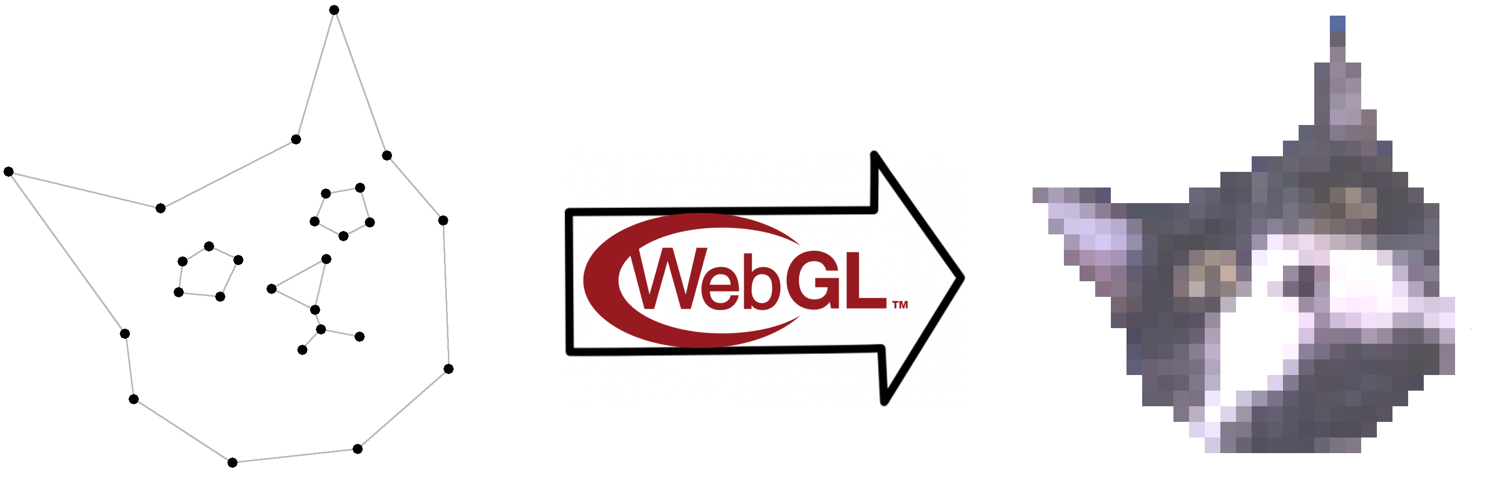
In this figure on the left: a vectorized cat. Each point is a vector encoding the position from the origin. Such an image can be scaled indefinitely, but cannot be displayed directly on the screen. On the right: a rasterized image formed by pixels.
As we already learned in the introduction, WebGL allows you to run heavily parallelized code by exploiting the rendering pipeline. However, unlike CUDA or OpenCL, WebGL unfortunately is not a general purpose computation pipeline for running parallelized code. Therefore, to benefit from the parallel GPU architecture, we need to transform all deep learning relevant operations into WebGL rendering pipelines. This should give you enough motivation to follow this section with enough attention to understand the basic principles of the rendering pipeline, shaders, and GLSL.
WebGL is standardized by the Khronos Group, like OpenGL. Its specifications are on https://www.khronos.org/registry/webgl/specs. WebGL output is rendered within the <canvas> element. So, the first step to play with WebGL is to insert a <canvas> element in the HTML code of the webpage:
<body><canvasid='myWebGLCanvas'height='512'width='512'></canvas></body>
After the page loads, get the canvas from the DOM in the JavaScript code and create the WebGL context GL. At this point check if the configuration of the user is compatible with WebGL:
varmyCanvas=document.getElementById('myWebGLCanvas');varGL;try{GL=myCanvas.getContext('webgl',{antialias:false,depth:false});}catch(e){alert('Cannot init a WebGL context. So sad...:(');}
We have disabled antialiasing and depth buffer because we are going to use WebGL for computing instead of rendering. After this operation, the <canvas> HTML element is fully dedicated to WebGL. It will not be possible to use it for canvas2D rendering or to unbind the WebGL context. In the following samples, the GL variable is the point of entry of the WebGL API: all WebGL functions and attributes are methods and properties of the context.
From a WebGL point of view, the drawing area is called the viewport. Its coordinate system always has the origin in the center, so the X axis goes from -1 (left) to 1 (right), and the Y axis goes from -1 (bottom) to 1 (top).
The WebGL workflow
The WebGL workflow is split between:
- The host code, running on the CPU and written in JavaScript. It is responsible to bind geometries and matrices to the GPU memory and handle the user interactions.
- The graphic code, running on the GPU and wrapped into small programs called the shaders. They are written in GLSL (Graphic Library Shading Language), a C-style language.
JavaScript is unable to parse GLSL natively, so the GLSL source code and variable names are always declared as strings and then passed to the WebGL context. This looks like a big drawback at first, however when working with Typescript, the usage of template strings will greatly improve the readability of GLSL shaders. However, for this book we will stick with JavaScript.
WebGL provides access to two kinds of shaders:
- The vertex shader takes the geometry data as input and transforms it. It operates on vertex data (the points of the vector geometries), which is stored in Vertex Buffer Objects (VBOs). This shader is executed before the rasterization process.
- The fragment shader is called once for each drawn pixel when antialiasing is disabled. It is executed after the rasterization process, which interpolates the vertex geometries for each output pixel. It is rendered once for each pixel and determines the output color of this pixel.
For example, if a 3D cube is drawn with WebGL:
- The vertex shader is executed once for each corner of the cube. It projects the 3D position to the viewport.
- The fragment shader applies the color for each drawn pixel.
A couple consisting of a shader of each type is called a shader program. It fully characterizes a specific rendering (i.e. a material for 3D rendering). Both shaders have the same structure:
//declaration of the I/O variables//custom functions//main loopvoidmain(void){//main code hereouput_variable=value;}
The output variable of the vertex shader is always gl_Position. It is a four dimensional vector [x,y,z,w] in clipping coordinates. The position of the point in 2D in the viewport is [x/w, y/w]. z/w is the depth buffer value, used in 3D rendering to manage depth overlapping. w is the extension of 3D coordinates to 4D homogeneous coordinates, a coordinate system that facilitates affine transformations (rotation, scaling and translation). Using homogeneous coordinates an affine transformation can be written in a single matrix multiplication.
The output variable of the fragment shader is gl_FragColor or gl_FragData depending on the GLSL version. It is the RGBA color value of the pixel, where A represents the alpha channel and hence manages transparency. For standard color rendering, each channel value is clamped between 0 and 1 (for example [1,1,1,1] is opaque white, [0.5,0,0,1] is 50% dark red and [1,0,0,1] is opaque black).
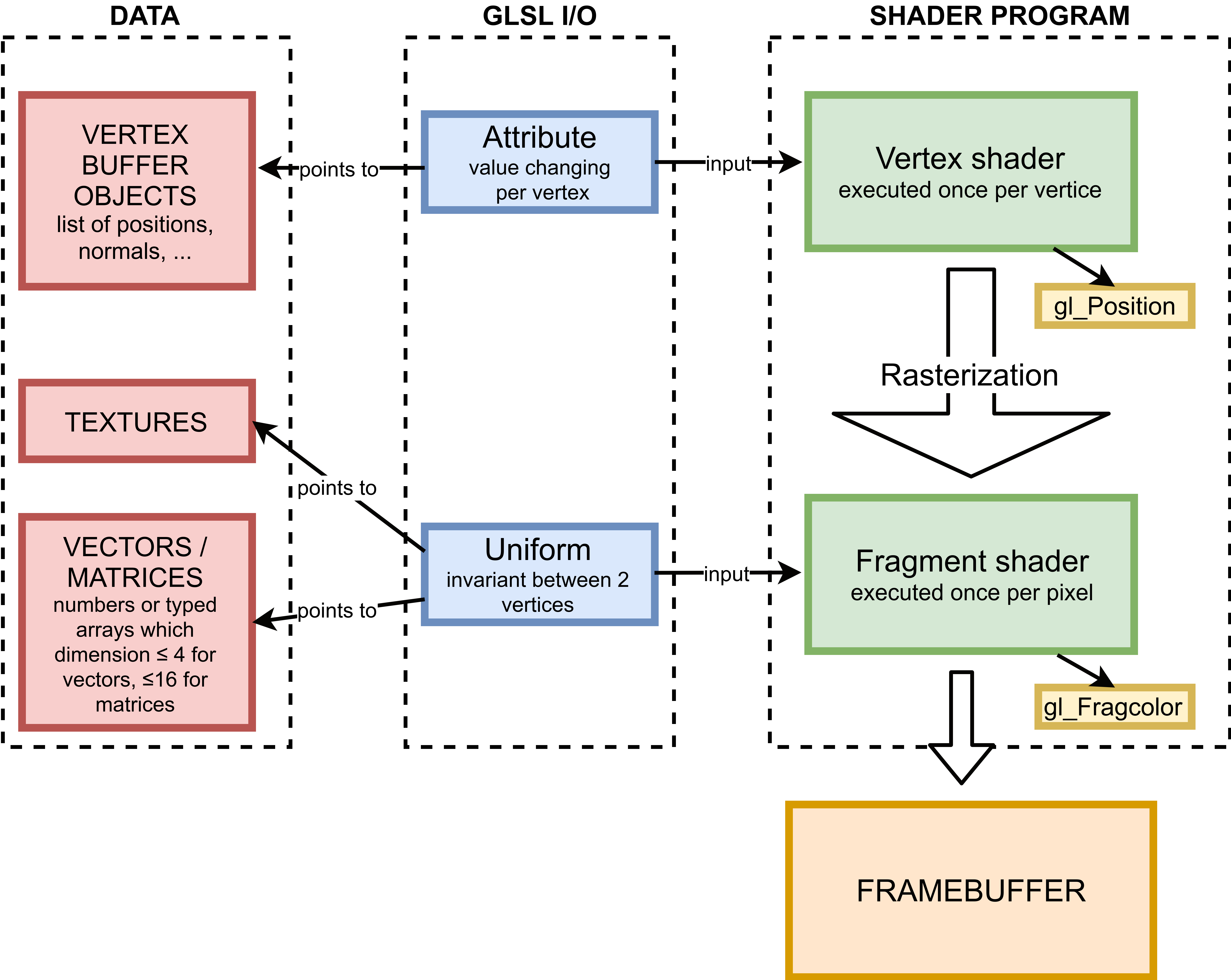
This figure is a simplified diagram of a WebGL workflow (we have deliberately forgotten the varying GLSL I/O type because they may not be used for GPGPU). On the left, there is the data: per vertex data for the VBOs, typed arrays for the textures or JavaScript numbers. In the middle there are the GLSL I/O variables: they are the bridge between JavaScript and GLSL. They are a kind of pointer in JavaScript, and they can be directly used in the shaders. On the left there is the GPU code. The rasterization process between the shaders is automatically done by the graphic drivers.
Fragment shader rendering
We use the main computations in the fragment shader. We fill the viewport with two triangles and we do all of the rendering in the fragment shader. This is common practice when using the WebGL shaders for computing. Using these two triangles will make sure that we can later execute one fragment shader per pixel. If the triangles don’t cover the whole viewport, the fragment shaders are only executed for the pixels covered by the triangle.
The WebGL workflow is still quite stiff and we cannot use the shaders separately. So we have to use the vertex shader too, but only to fill the viewport with two triangles. Then the color of each pixel of the triangles is assigned in the fragment shader. Later we will replace rendering by computing. We refer to the first example of the book code repository: chapter3/0_webglFirstRendering.
The Vertex buffer objects
We declare a JavaScript typed array containing the 2D coordinates of the four corners of the viewport:
varquadVertices=newFloat32Array([-1,-1,//bottom left corner -> index 0-1,1,//top left corner -> index 11,1,//top right corner -> index 21,-1//bottom right corner-> index 3]);
Then, group these four points to build two non overlapping triangles using the indices of the vertices:
varquadIndices=newUint16Array([0,1,2,//first triangle if made with points of indices 0,1,20,2,3//second triangle]);
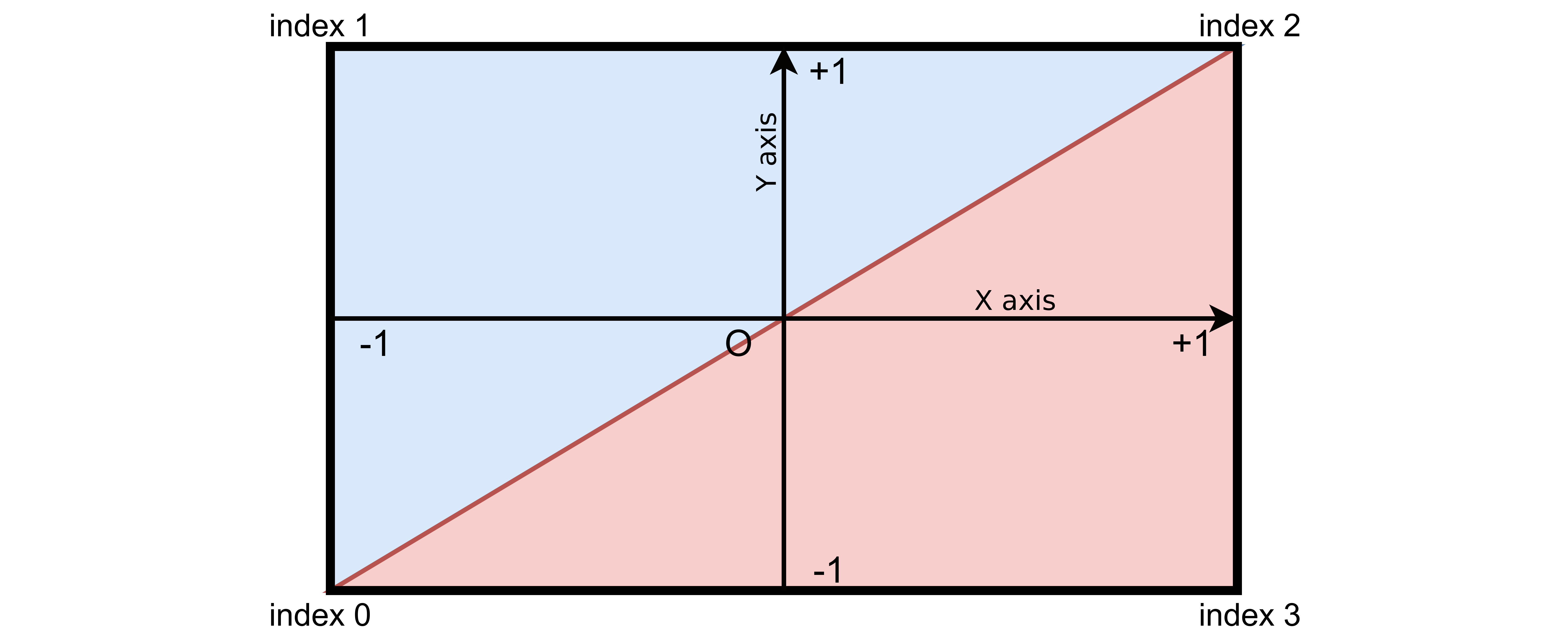
In this figure the two triangles fill the viewport. The top left triangle is displayed in blue. Its point indices are 0,1,2. The red bottom right triangle, which point indices, are 0,2,3.
The data is stored in JavaScript typed arrays. We send them to the GPU memory (the VRAM) by creating Vertex Buffer Object (VBO). A VBO is simply an array stored in the GPU memory:
//send vertices to the GPU:varquadVerticesVBO=GL.createBuffer();GL.bindBuffer(GL.ARRAY_BUFFER,quadVerticesVBO);GL.bufferData(GL.ARRAY_BUFFER,quadVerticesVBO,GL.STATIC_DRAW);//send indices to the GPU:varquadIndicesVBO=GL.createBuffer();GL.bindBuffer(GL.ELEMENT_ARRAY_BUFFER,quadIndicesVBO);GL.bufferData(GL.ELEMENT_ARRAY_BUFFER,quadIndicesVBO,GL.STATIC_DRAW);
The shader program
The vertex shader takes the quad vertices as input, and outputs them at the corners of the viewport. Here is the source code of the vertex shader in GLSL:
attributevec2position;voidmain(void){gl_Position=vec4(position,0.,1.);//position in clip coords}
As you can see in the above example, we only need the x and y coordinates of the vertices. Hence we set the depth z=0 and w=1.
Then we write a fragment shader, which outputs the 2D position of each pixel in the viewport in the red and green color channels. From now on, we will often use this trick to encode data in the color channels of the output pixels.
precisionhighpfloat;uniformvec2resolution;//resolution in pixelsvoidmain(void){//gl_FragCoord is a built-in input variable.//It is the current pixel position, in pixels:vec2pixelPosition=gl_FragCoord.xy/resolution;gl_FragColor=vec4(pixelPosition,0.,1.);}
We declare both shaders as JavaScript strings and we compile them separately:
//declare shader sources as stringvarshaderVertexSource="attribute vec2 position; "+"void main(void){ "+"gl_Position=vec4(position, 0., 1.); "+"}";varshaderFragmentSource="precision highp float; "+"uniform vec2 resolution; "+"void main(void){ "+"vec2 pixelPosition=gl_FragCoord.xy/resolution; "+"gl_FragColor=vec4(pixelPosition, 0.,1.); "+"}";//function to compile a shaderfunctioncompile_shader(source,type,typeString){varshader=GL.createShader(type);GL.shaderSource(shader,source);GL.compileShader(shader);if(!GL.getShaderParameter(shader,GL.COMPILE_STATUS)){alert("ERROR IN "+typeString+" SHADER: "+GL.getShaderInfoLog(shader));returnfalse;}returnshader;};//compile both shaders separatelyvarshaderVertex=compile_shader(shaderVertexSource,GL.VERTEX_SHADER,"VERTEX");varshaderFragment=compile_shader(shaderFragmentSource,GL.FRAGMENT_SHADER,"FRAGMENT");
We create the shader program, which contains all of the graphic code for a specific rendering:
varshaderProgram=GL.createProgram();GL.attachShader(shaderProgram,shaderVertex);GL.attachShader(shaderProgram,shaderFragment);
Finally, we link GLSL I/O variables with JavaScript pointers-like variables, which will be used later to update GLSL values from JavaScript. GLSL variable names are always given as string because JavaScript cannot understand GLSL:
//start the linking stage:GL.linkProgram(shaderProgram);//link attributes:varposAttribPointer=GL.getAttribLocation(shaderProgram,"position");GL.enableVertexAttribArray(posAttribPointer);//link uniforms:varresUniform=GL.getUniformLocation(shaderProgram,"resolution");
Rendering time
The only VBO used in GPGPU is the quad, so we can bind it to the context once and for all:
GL.bindBuffer(GL.ARRAY_BUFFER,quadVerticesVBO);GL.vertexAttribPointer(posAttribPointer,2,GL.FLOAT,false,8,0);GL.bindBuffer(GL.ELEMENT_ARRAY_BUFFER,quadIndicesVBO);
The drawcall GL.vertexAttribPointer details how to parse shader program attributes from VBO data. It means that the posAttribPointer attribute (previously linked to GLSL "position" variable) has two components that type is GL.FLOAT. false disables on a fly vertex normalization, 8 is the size of 1 vertice in bytes (8 bytes = 2 components * 4 bytes because a GL.FLOAT element is stored using 4 bytes).
Let’s trigger the rendering:
GL.useProgram(shaderProgram);//update GLSL "resolution" value in the fragment shader:GL.viewport(0,0,myCanvas.width,myCanvas.height);//update GLSL "resolution" value in the fragment shader:GL.uniform2f(resUniform,myCanvas.width,myCanvas.height);//trigger the rendering:GL.drawElements(GL.TRIANGLES,6,GL.UNSIGNED_SHORT,0);GL.flush();

Understanding the GPU power
Each pixel color value is assigned in parallel by the fragment shader statement gl_FragColor=vec4(pixelPosition, 0.,1.). Each pixel only knows its relative position given by built-in variable gl_FragCoord. This is the power of WebGL parallelization. The resulting pixel array materialized by the rendering is analogous to a CUDA kernel.
Replace the main function of the fragment shader by:
voidmain(void){vec2pixPos=gl_FragCoord.xy/resolution;//translate and scale:vec2pixPosCentered=1.3*(pixPos*2.-vec2(1.55,1.));vec2z=pixPosCentered,newZ;floatj=0.;for(inti=0;i<=200;i+=1){newZ=pixPosCentered+vec2(z.x*z.x-z.y*z.y,2.*z.y*z.x);if(length(newZ)>2.)break;z=newZ;j+=1.;}//generate RGB color from j:vec3color=step(j,199.)*vec3(j/20.,j*j/4000.,0.);gl_FragColor=vec4(color,1.);}
We get this beautiful Mandelbrot fractal so fastly that it could be done inside a rendering loop running smoothly at 60 frames per second. You can try it on the github repository, chapter3/1_mandelBrot.
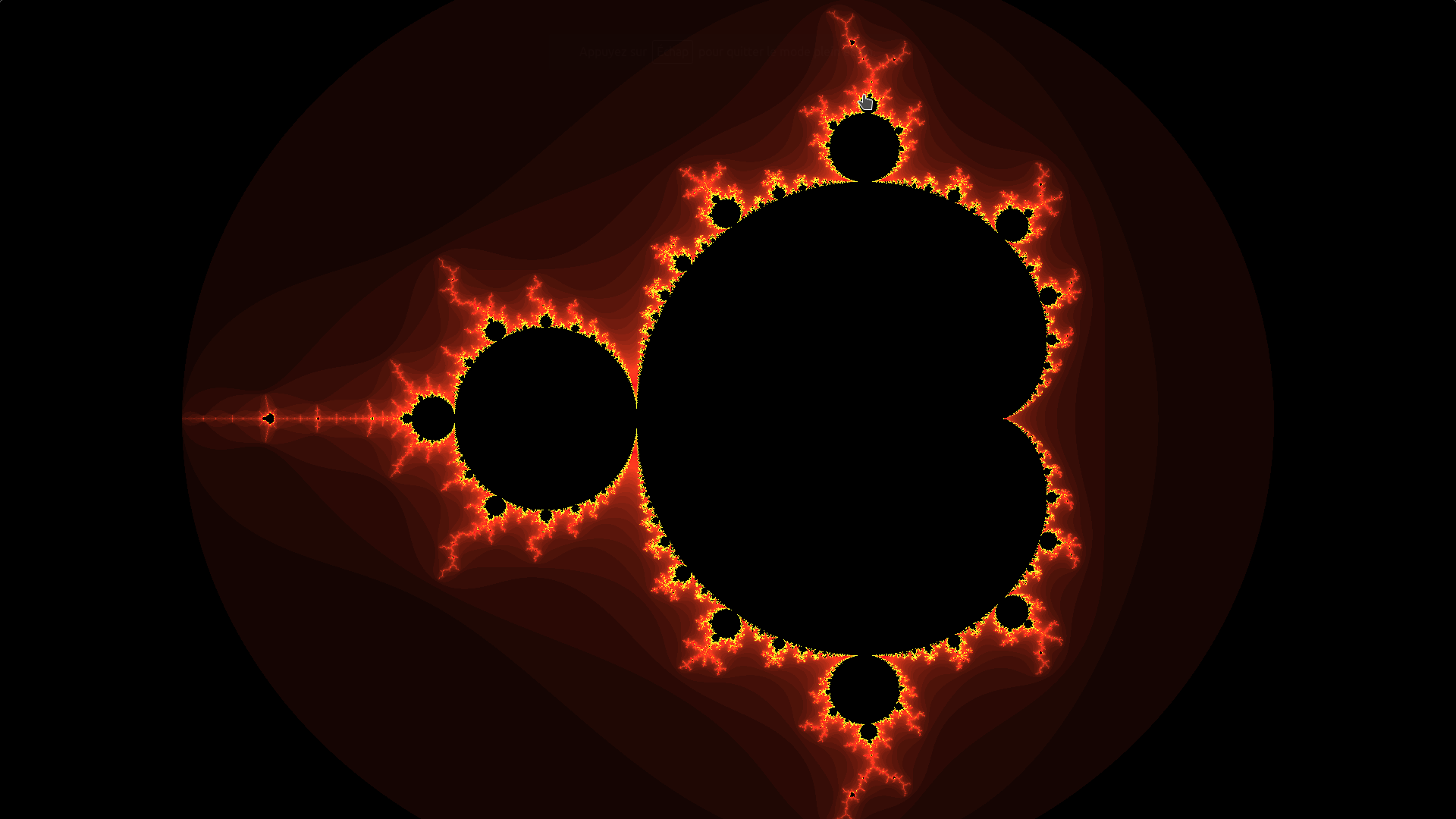
Explanations about this fractal can be found on nuclear.mutantstargoat.com. Many interesting renderings can be obtained by using only the fragment shader, including real-time raytracing implemented with the raymarching algorithm. They can be found on shadertoy.com.
General purpose computing with WebGL
Instead of drawing beautiful color gradients or fractals using the fragment shader, we will process computations. In this part, the main principles of general purpose computing with WebGL (GPGPU) are explained.
We can perform computations in parallel in two different places with WebGL: in the fragment shader or in the vertex shader. It is not convenient to process the main workload in the vertex shader because its output gl_Position can’t be read directly or saved into a texture or another object like gl_FragColor. It controls the position, so if some computation results have the same position in the viewport, they will overlap, and if they fall outside of the viewport they won’t be readable. Moreover, we usually deal with less vertices than output pixels and hence parallelization in the fragment shader will be much more efficient.
Furthermore, we would still end up reading or saving this result by using the output of the fragment shader. So for GPGPU we always use the vertex shader to simply fill the viewport and do the whole computational part in the fragment shader.
Instead of rendering on the HTML canvas and to the screen, we render to a so called framebuffer, which is a location within the GPU memory. In the next drawcall, use this framebuffer as a texture and read its values from another fragment shader. Although a texture is usually seen as an image stored in the VRAM, apprehend it as a 2D array with four channels per value (which are the RGBA color channels). It stores the result of a calculation step and the 4 channels are assigned according to an arbitrary convention.
This is a kind of old school GPGPU, because there was the release of GPU specific computation libraries or APIs like OpenCL or CUDA.
Popular JavaScript libraries for deep learning in the browser (such as Tensorflow.js) map whole deep learning models into the VRAM. Each layer’s output is written into a texture and fed into the next layer where it is looked up in the next fragment shader. We want to avoid reading the GPU memory from the main JavaScript thread at all costs, but rather build the complete execution graph of the deep learning model as a giant render path.
Debugging WebGL
WebGL can be hard to debug because the code is executed on different supports and there are important variations between graphic hardware. Some browser extensions like WebGL inspector or WebGL Insight can help to inspect the graphic memory linked to a specific WebGL context. It is possible to browse and inspect the textures, the VBOs, or to list the drawcalls.
Hardware dependent errors
If you face a hardware dependant bug, you can:
- Open chrome://gpu to collect information about Chrome WebGL support.
- Visit webglreport.com at http://webglreport.com/ to collect information about WebGL1 and 2 support, extensions, and graphic hardware limitations.
If WebGL does not work anymore on a specific configuration, the graphic drivers may have been blacklisted by the browser because a security hole has been discovered. Their update should fix the problem.
GLSL syntax errors
GLSL syntax errors are detected when shaders are compiled. They are explicit and the line number (in the GLSL code) is specified so they are easy to fix. When working with shaders, this error is most common.
WebGL runtime error
Most often these errors are reported as warnings in the standard JavaScript console. They can occur, for example, if a custom framebuffer is not bound to a texture, or if a texture is initialized from a typed array which has a different length than expected. The error message is explicit, but the JavaScript line number where there is the drawcall triggering the error is not specified.
You can set a breakpoint and analyze the error in the JavaScript console. We advise to add the GL.finish() statement before the breakpoint in order to be sure that the GPU has executed all its pending drawcalls.
Algorithmic errors
These errors are hard to analyze because it is impossible to set a breakpoint in the shaders. A specific rendering needs to be implemented to highlight the problem by displaying the simulation variables in the color channels of the standard framebuffer.
Render to texture
We develop a Conway game of life to illustrate the concept of render to texture for computing. WebGL and full JavaScript implementations of this simulation are included in the code repository of this book. The WebGL program is about 4000 times faster running on low level graphic hardware and a high end CPU. It is a wonderful example to illustrate the effects of parallelization on a relatively simple code. The source code is available on the Github repository, chapter3/2_renderToTexture.
We first declare the global parameters of the simulation:
varSETTINGS={simuSize:256,//simulation is done in a 256*256 cells//squarenIterations:2000//number of computing iterations};
A default framebuffer object (FBO) is created and bound to the context when the WebGL context is instantiated. The rendering occurs in this framebuffer which controls the display. To render to texture (RTT), we need to create a custom framebuffer object. Then we bind it to the context:
varrttFbo=GL.createFramebuffer();GL.bindFramebuffer(GL.FRAMEBUFFER,rttFbo);
This function creates a texture from a JavaScript typed array:
functioncreate_rttTexture(width,height,data){vartexture=GL.createTexture();GL.bindTexture(GL.TEXTURE_2D,texture);//texture filtering://pick the nearest pixel from the texture UV coordinates//(do not linearly interpolate texel values):GL.texParameteri(GL.TEXTURE_2D,GL.TEXTURE_MAG_FILTER,GL.NEAREST);GL.texParameteri(GL.TEXTURE_2D,GL.TEXTURE_MIN_FILTER,GL.NEAREST);//do not repeat texture along both axis:GL.texParameteri(GL.TEXTURE_2D,GL.TEXTURE_WRAP_S,GL.CLAMP_TO_EDGE);GL.texParameteri(GL.TEXTURE_2D,GL.TEXTURE_WRAP_T,GL.CLAMP_TO_EDGE);//set size and send data to the texture:GL.texImage2D(GL.TEXTURE_2D,0,GL.RGBA,width,height,0,GL.RGBA,GL.UNSIGNED_BYTE,data);returntexture;}
It is not possible to simultaneously read a texture and render to it. So we need to create two textures. Both store the cell states in the red channel only (the cell is alive if the red channel value is 1.0 and dead if it is equal to 0.0):
vardataTextures=[create_rttTexture(SETTINGS.simuSize,SETTINGS.simuSize,data0),create_rttTexture(SETTINGS.simuSize,SETTINGS.simuSize,data0)];
data0 is a randomly initialized Uint8Array storing the RGBA values of the texture.
During the first simulation iteration, we render to dataTextures[1] using dataTextures[0], and then we swap the two textures and reiterate.
We need two shader programs:
- The computing shader program takes the cell states texture as input and returns the updated cell states.
- The rendering shader program was used once at the end of the simulation to display the result on the canvas.
Both shader programs have the same vertex shader, still drawing two triangles to fill the viewport. All the logic is done by the fragment shader.
This is the main function of the computing fragment shader. It implements the logic of the Conway game of life:
voidmain(void){//current position of the rendered pixel:vec2uv=gl_FragCoord.xy/resolution;vec2duv=1./resolution;//distance between 2 texels//cellState values: 1->alive, 0->dead:floatcellState=texture2D(samplerTexture,uv).r;//number of alive neighbors (Moore neighborhood):floatnNeighborsAlive=texture2D(samplerTexture,uv+duv*vec2(1.,1.)).r+texture2D(samplerTexture,uv+duv*vec2(0.,1.)).r+texture2D(samplerTexture,uv+duv*vec2(-1.,1.)).r+texture2D(samplerTexture,uv+duv*vec2(-1.,0.)).r+texture2D(samplerTexture,uv+duv*vec2(-1.,-1.)).r+texture2D(samplerTexture,uv+duv*vec2(0.,-1.)).r+texture2D(samplerTexture,uv+duv*vec2(1.,-1.)).r+texture2D(samplerTexture,uv+duv*vec2(1.,0.)).r;if(nNeighborsAlive==3.0){cellState=1.0;//born}elseif(nNeighborsAlive<=1.0||nNeighborsAlive>=4.0){cellState=0.0;//die};gl_FragColor=vec4(cellState,0.,0.,1.);}
The texture2D statement fetches a pixel from a texture (also called a texel). Its arguments are the texture sampler and the texel coordinates. We can use around 16 textures simultaneously in one fragment shader, depending on the GPU capabilities. The exact number can be obtained by the statement GL.getParameter(GL.MAX_TEXTURE_IMAGE_UNITS). Of course you can instantiate many more textures but you won’t be able to use them all simultaneously. A sampler has the type uniform sampler2D in the shaders but is assigned like an integer from JavaScript:
//At the linking stepvar_samplerTextureRenderingUniform=GL.getUniformLocation(shaderProgramRendering,'samplerTexture');//...//We affect the sampler value to channel 7, like an integerGL.useProgram(myShaderProgram);GL.uniform1i(_samplerTextureRenderingUniform,7);//...//Just before the rendering://we activate the texture channel 7:GL.activeTexture(GL.TEXTURE7);//we bind myTexture to the activated channel:GL.bindTexture(GL.TEXTURE_2D,myTexture);
The second parameter of the GLSL statement texture2D are the textures coordinates, also called UV coordinates. It is a vec2 instance, which locates the fetched texel. Its components are both between 0.0 and 1.0.
Let’s prepare the simulation step:
GL.useProgram(shaderProgramComputing);GL.viewport(0,0,SETTINGS.simuSize,SETTINGS.simuSize);
And launch the simulation loop:
for(vari=0;i<SETTINGS.nIterations;++i){//dataTextures[0] is the state (read):GL.bindTexture(GL.TEXTURE_2D,dataTextures[0]);//dataTextures[1] is the updated state (written):GL.framebufferTexture2D(GL.FRAMEBUFFER,GL.COLOR_ATTACHMENT0,GL.TEXTURE_2D,dataTextures[1],0);GL.drawElements(GL.TRIANGLES,6,GL.UNSIGNED_SHORT,0);dataTextures.reverse();}
The instruction GL.framebufferTexture2D(...) means that everything that is drawn on the current bound framebuffer (which is rttFbo) is also drawn into the texture dataTextures[1].
Finish by the rendering step:
//come back to the default FBO (displayed on the canvas):GL.bindFramebuffer(GL.FRAMEBUFFER,null);GL.useProgram(shaderProgramRendering);GL.viewport(0,0,myCanvas.width,myCanvas.height);//[...]//trigger the rendering:GL.drawElements(GL.TRIANGLES,6,GL.UNSIGNED_SHORT,0);GL.flush();
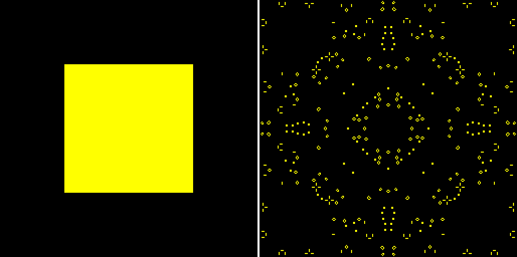
This figure is a Conway game of life simulation. We have changed the cell initialization values from the repository code to start with a square of living cells at the center of the simulation area (left image). After 2000 iterations, the complexity emerges (right image).
Precision matters
We only use discrete values in the Conway game of life: the cell is either alive or dead. But if you need to use continuous values, you would be limited by the WebGL default eight bits precision. Indeed, each component of gl_FragColor is encoded using eight bits, and is clamped between 0 and 1. There are only 2^8 = 256 possible values for each component. This is far enough to encode a color because human eye is not accurate enough to distinguish between two colors differing at one bit. But we need higher precision for deep learning models because we usually deal with floating-point values. 16 bits (GL.HALF_FLOAT) would be enough, but on some configurations only 32 bits precision (GL.FLOAT) is available. These capabilities are required:
- instantiate
FLOATorHALF_FLOATtextures - render to texture to
FLOATorHALF_FLOATtextures
If you use WebGL1, you need to enable OES_TEXTURE_FLOAT or OES_TEXTURE_HALF_FLOAT extensions (which are not always implemented). Then you still need to test render to FLOAT or HALF_FLOAT textures.
If WebGL2 is used, these requirements are met because FLOAT and HALF_FLOAT have been included in the specifications. But only render to texture to HALF_FLOAT texture is specified. WebGL2 is backward compatible with WebGL1 and can be used by:
varGL=myCanvas.getContext('webgl2',...);
At the initialization of the context, you should:
- If WebGL2 is available, use WebGL2 with a
HALF_FLOATprecision If WebGL1 is available:
- get the
OES_TEXTURE_FLOATextension - test RTT with
FLOATtextures
- get the
- If the
OES_TEXTURE_FLOATextension is not available or if RTT does not work:- get the
OES_TEXTURE_HALF_FLOATextension - test RTT on it
- get the
On some GPU configurations, we also have to get the <WEBGL|EXT|OES>_color_buffer_float extension. Otherwise it is not possible to bind a framebuffer object to a FLOAT or HALF_FLOAT texture.
The precision used in a shader is specified in the first line by:
precisionhighpfloat
It accepts three values:
lowp: computations are done with eight bit precision. It is fast, but this is not precise enough for floating-point number calculations. It still suits for rendering color values.mediump:highp,lowpor another precision between the two is used depending on the GPU configuration. It is important to check the real precision usingGL.getShaderPrecisionFormat(GL.MEDIUM_FLOAT)before using it because this level of precision can vary a lot depending on the graphic hardware.highp: floating-point numbers are manipulated using 16 or 32 bits. 16 bits are enough for deep learning computations (but not always for physical simulations...). The real precision for this level can be checked by runningGL.getShaderPrecisionFormat(GL.HIGH_FLOAT).
The returned value of GL.getShaderPrecisionFormat(<level>) is an object that the precision property equals to the number of bits encoding the fraction of a floating-point number in the shaders. For example, for a 32 bits floating-point number it is 23, for a 16 bits floating-point number it is 10.
Start from the Conway game of life to develop a heat simulation, involving render to floating-point textures. You can test it on the Github repository, chapter3/3_RTTfloat. We simulate in 2D a square part of iron, which side measures 2.56 meters heated at 100°C, surrounded by iron at 0°C. The heat diffuses over time.
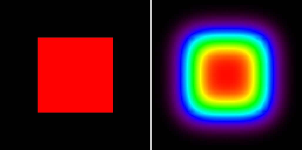
In this figure, on the left: a simulation in the initial state, and on the right: a simulation after 2000 seconds. Colors are defined by the IDL_Rainbow color map implemented in the fragment shader and calibrated from 0°C to 100°C.
Optimizations
Implementing a deep learning network with WebGL is not easy and it introduces a lot of complexity due to the specific workflow and the different execution paths depending on the graphic hardware. The only goal is to increase the performance, and that would be a shame to undermine this effort by falling into common graphic programming pitfalls.
Futhermore, speed really matters in many cases. Computer vision problems, such as an image classification, segmentation, or object detection, often run on continuous video streams where we have around hundred milliseconds to run at least at 30 Frames Per Second (FPS). Therefore, you should follow a few rules on basic shader optimizations.
GLSL development
As you can imagine, GLSL development can be the subject of an entire book (the most popular ones cover more than 1.000 pages!). We will only deal with most common and penalizing development mistakes. If you want to go further with WebGL and GLSL learning you can try the free interactive tutorials of http://webgl.academy.
When possible, avoid conditional statements like if...then...else in the shaders. Consider this code computing an exponential linear unit (ELU) activation function:
floatELU(floatx){if(x>=0.0){returnx;}else{returnexp(x)-1.0;}}
It uses an if statement. This code is more efficient:
floatELU(floatx){returnmix(exp(x)-1.0,x,step(x,0.));}
The GLSL built-in mix() function is defined by: mix(x,y,a)=x*(1-a)+y*a.
Use several small shaders instead of one large shader. If the shader is too long, the GPU execution cache will have to be updated during execution time, and this is penalizing.
Beware of floating-point specials
In a high precision shader, floating-point numbers are stored using 16 to 32 bits, depending on the GPU. The first bit determines the sign, then for a 32 bits float, 8 bits encodes the exponent and 23 bits the fraction. Because of this storage format, the maximum value of a 32 bits encoded float is 3.4e38, and the minimum is -3.4e38. For 16 bits floating-point numbers, this range is narrower.
](http://images-20200215.ebookreading.net/12/2/2/9781939902542/9781939902542__deep-learning-in__9781939902542__assets__float32.png)
This figure is a 32 bit standard floating-point number binary encoding. Source: Wikipedia.
If the result of a computation above is this maximum value, it is replaced by a floating-point special, +Infinite. The handling of floating-point specials like +Infinite, -Infinite, NaN, depends on the GPU hardware. Then this value may propagate along the computation stream.
Floating-point specials can be stored on FLOAT or HALF_FLOAT textures. So if we render to texture, these values may propagate over the following calculation passes.
Floating-point specials appear even if the calculation step is implicit. We consider the GLSL function computing the ELU activation function:
floatELU(floatx){returnmix(exp(x)-1.0,x,step(x,0.));}
If x=100, which is not unrealistic (x can be the summed weighted inputs of the neuron), we get ELU(100) = 100. But the GPU has to compute ELU(100) = mix(exp(100)-1, 100, 1) = (exp(100)-1) * 0 + 100. But exp(100) = 2.7.10^{43} is above the maximum floating-point number value. So it is replaced by a floating-point special, +Infinity. And exp(100)-1 = +Infinity-1 = +Infinity. The GPU compute ELU(100) = +Infinity * 0 + 100 . But +Infinity * 0 is undefined and it generates another floating-point special, NaN. NaN always propagates along the computation flow because any operation involving NaN outputs NaN (On the contrary Infinity can disappear because 1/Infinity = 0). The GPU outputs ELU(100) = NaN + 100 = NaN. Then all connected neurons of the next layer receive a NaN value among their inputs, and will output NaN too and so on...
There are some solutions to avoid floating-point specials:
- Avoid functions involving exponentials (e.g. softmax) or logarithms. Sometimes they can be replaced by polynomial approximations over finite intervals.
- If
mix()or other GLSL interpolation function is called, make sure that both terms are small enough. This implementation of ELU is safer:
floatELU(floatx){returnmix(exp(-abs(x))-1.0,x,step(x,0.));}
- Majorate or minorate.
- Use deep learning techniques to keep the weights and bias at low values, like L1 or L2 regularization.
All specifications about floating-point specials on Nvidia GPUs can be found on the Nvidia Website.
Take account of texture cache
A GPU has a hierarchical cache system like a CPU. When a texel is fetched with a texture2D() statement in the fragment shader, the GPU searches first in the faster, but smaller levels of cache. If it is not here, it triggers a cache miss and searches in the second cache, larger but slower, and so on until it fetches it directly in the highest level of texture cache. Then the texel is copied in a lower level of cache, and will be faster to retrieve for the next lookups.
If neighboring pixels of the rendering reuse the same texels, the cache misses rate is low and the shader runs fast. But if they use many different texels, so many cache misses will occur, and the performance will strongly decrease. In some cases there are several ways to arrange the data in a texture. One of the alternatives is often better optimized for this aspect.
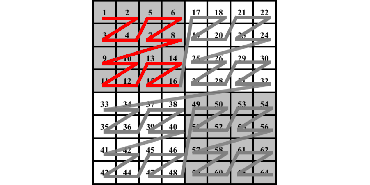
In this figure you see the graphic memory, where texels are not aligned but sorted with the Morton order. This process is called texture swizzling. When a texel is fetched, the whole line of texels (displayed in red) is pushed to a low level of the GPU memory cache. So the 2D neighboring texels will be faster to fetch, because they are already in the low levels of memory cache.
Although there are several publications about texture caches (Texture Caches, Michael Doggett, Lund University), the cache implementation depends a lot on the hardware. It is still necessary to test WebGL programs with a sample of different hardware to make sure that it is fast enough and runs everywhere.
The color channels role
Render to texture is defined for four color channels textures and four color channels framebuffers. They can be used in different ways:
- Only 1 channel can be used like in our Conway game simulation. But it is not optimal because the GPU anyway processes four component vectors and matrices at once, so we could do four times more calculations for the same execution duration.
- Each 32 bits value can be packed into four RGBA eight bits components. It is then possible to not use floating-point textures at all. The main drawback is that each fragment shader should unpack the RGBA input values from textures to 32 bits values, then to pack the output value into the eight bits RGBA channels of
gl_FragColor. - Four neuron networks can run in parallel, one per RGBA channel. They have learned with different initialization parameters and their outputs are slightly different. Then the final output is averaged over the four neuron networks. These four channels help to reduce the output noise.
Disable dithering
The WebGL state can be modified using GL.enable() or GL.disable() instructions. Their effect is retentive so the state of the WebGL context needs to be changed once. Dithering should be disabled when the fragment shader is used for computing, because it may alter the output values. It consists in applying some noise to the fragment shader output to avoid color quantization visual artifacts.
GL.disable(GL.DITHER);

In this figure you see how dithering may alter color pixel values in the framebuffer if it has lower precision than the computed colors. On the left: a picture of a cat in 32 bit RGBA colors. In the middle: a picture of the cat in 2 bit indexed RGBA color. Color precision has decreased and each pixel is replaced by the nearest color in the new color palette. On the right: a picture of the cat with the same 2 bit indexed RGBA color, but with dithering enabled. Pixel colors are no longer the nearest color in the new color palette: some noise has been introduced in order to avoid the creation of borders.
Avoid framebuffer switches
It is far more efficient to instantiate one framebuffer and to dynamically bind a texture on it using GL.framebufferTexture2D each time we need to render to a specific texture than instantiating one framebuffer per texture, to bind each texture to a different framebuffer, and to dynamically switch the framebuffer when we need to render to the bound texture using GL.bindFramebuffer. Indeed, GL.bindFramebuffer is very costly in terms of performance.
One triangle is better than two
Rather than drawing two triangles filling the viewport, we can draw only one triangle larger than the viewport (its corners can be [-1,-1], [3,-1], [-1,3]). It is slightly faster. The fragment shader is still executed once per pixel thanks to the scissor test, integrated in the WebGL graphic pipeline and enabled by default.
From CPU to GPU and vice versa
In the beginning, the data are processed by JavaScript, whether it is images, video, or arrays. So they are stored in the RAM and in the CPU registers, and they are handled by the CPU. Then they are sent on the GPU and processed with the shaders. At the end, we will probably need them on the CPU side again. So we need to transfer the data from the CPU to the GPU, then do the opposite.
floating-point texture initialization
floating-point textures are often initialized from JavaScript data. For example, if synaptic weights are stored in a texture, we fill it from a JavaScript array of values calculated during a previous training or matching a specific random distribution. If the texture stores GL.FLOAT elements (using 32 bits per float), the initialization is straightforward:
//small variation between WebGL1 and 2:varinternalPixelFormat=(ISWEBGL2)?GL.RGBA32F:GL.RGBA;GL.texImage2D(GL.TEXTURE_2D,0,internalPixelFormat,<width>,<height>,0,GL.RGBA,GL.FLOAT,<instance_of_Float32Array>);
But the initialization from an array is more difficult if the texture stores GL.HALF_FLOAT elements, because there is no JavaScript Float16Array type. On JavaScript side, we have to encode the floating-point values with 16 bits per value using the standard float16 encoding (one bit for the sign, five for the exponent and 10 for the fraction). Then we have to put the encoded values into a JavaScript Uint16Array. The encoding function from JavaScript Float32Array to Uint16Array is provided in the code repository of this book (see RTTfloat heat simulation). Then we initialize the texture with the Uint16Array:
//see "continuous simulation" example to see the code//of the "convert_arrayToUInt16Array" function:varu16a=convert_arrayToUInt16Array(<instance_of_Float32Array>);varinternalPixelFormat=(ISWEBGL2)?GL.RGBA16F:GL.RGBA;GL.texImage2D(GL.TEXTURE_2D,0,internalPixelFormat,<width>,<height>,0,GL.RGBA,GL.HALF_FLOAT,u16a);
Get back computation results on CPU
Unless we have a 100% GPU workflow, at some point we need to get back our computation data to JavaScript. This operation is slow and it should be done as little as possible. We have to render into the default framebuffer (displayed on the <canvas> element), then to read the pixels using the instruction GL.readPixels. It fills a Uint8Array JavaScript typed array with the interleaved RGBA values of the pixels of a rectangular area. The slowness comes from the forced synchronization between the CPU and the GPU. Before using it we should create the WebGL context with the option preserveDrawingBuffer: true.
Reading eight bits encoded values is straightforward: the texture is rendered by a fragment shader, which copies the texture value to gl_FragColor. Then framebuffer values are read using GL.readPixels. But for floating-point value textures this is more complicated. We need to develop a specific fragment shader to pack each floating-point value into several eight bits values, then process several renderings with staggered viewports, read the renderings with one GL.readPixels drawcall and finally reconstruct the floating-point array from the Uint8Array with JavaScript.
The shader packing floats into eight bits color values is provided in the book repository, with an example of floating-point texture reading.
Texture and Shaders for Matrix Computation
After this ride into the fascinating world of WebGL GPGPU, we come back to deep learning to build a minimalist WebGL linear algebra library called WGLMatrix. Then we will use it to implement a simple neural network (not convolutional) learning to recognize handwritten digits from the MNIST dataset. A test of the first version of the linear algebra library is included in chapter3/4_WGLMatrix.
Standard matrix addition
There are built-in matrix types in GLSL only for matrices with largest dimensions less or equal to four. This is not enough for deep learning. So matrices are stored using textures and we need to develop specific shaders for common matrix operations. Each texel is a matrix entry, and the texture has the same resolution than the matrix dimensions.
When a matrix is created, if four JavaScript initialization arrays are provided, the RGBA channels are filled with them. Otherwise, if only one array is provided, its values are duplicated four times to fill the color channels. Each common matrix operation is done separately for the four RGBA channels. It is as if we process it four times in parallel with four different matrices.
The addition fragment shader does not depend on the matrix size like all other elementwise operators. This is its GLSL code:
voidmain(void){vec2uv=gl_FragCoord.xy/resolution;vec4matAValue=texture2D(samplerTexture0,uv);vec4matBValue=texture2D(samplerTexture1,uv);gl_FragColor=matAValue+matBValue;}
Standard matrix multiplication
Unlike the addition shader, the multiplication shader involves a for loop to iterate over a row of the first matrix and simultaneously over a column of the second matrix. With WebGL1, it is not possible to use non-constant values among for conditions. This restriction includes GLSL uniforms values or previous computation results. So, we need to compile one shader program per matrix common multiplication dimension. For example, this shader can be used for all multiplications between a (n, 10) matrix and a (10, m) matrix:
//vector between 2 consecutive texels of first factor:constvec2DU=vec2(1./10.,0.);//vector between 2 consecutive texels of second factor:constvec2DV=vec2(0.,1./10.);voidmain(void){vec2uv=gl_FragCoord.xy/resolution;vec2uvu=uv*vec2(1.,0.);vec2uvv=uv*vec2(0.,1.);vec4result=vec4(0.,0.,0.,0.);for(floati=0.0;i<10.0;i+=1.0){result+=texture2D(samplerTexture0,uvv+(i+0.5)*DU)*texture2D(samplerTexture1,uvu+(i+0.5)*DV);}gl_FragColor=result;}
We add 0.5 to i to pick the middle of the pixel, otherwise we may have a rounding error for some specific matrix dimensions. With WebGL2, non-constant for loop conditions have been implemented. But this is still not acceptable to only support WebGL2 for commercial applications (the support rate is 41% in March 2018, source: webglstats.com). So we build a WebGL1 shader, which also works for WebGL2.
We often have to simultaneously multiply and add matrices. For example, when we multiply a neuron layer inputs X by the weights matrix W, and then we add the biases B to compute the summed inputs Z: Z = WX + B. We should compile a specific shader to do this operation which is called FMA (Fused Multiply–Accumulate). It will save some render to texture passes.
Our matrix library, WGLMatrix, manages a dictionary of multiplication and FMA shader programs. If we need to process two matrices, which common dimension is included into the dictionary, we just use the shader program from the dictionary. Otherwise a new dimension specific shader program is compiled and added to the dictionary.
Activation function application
A shader is dedicated to the application of the activation function. We should be careful of floating-point specials, especially if the activation function involves exponentials or logarithms. This shader applies a sigmoid activation function:
constvec4ONE=vec4(1.,1.,1.,1.);voidmain(void){vec2uv=gl_FragCoord.xy/resolution;vec4x=texture2D(samplerTexture0,uv);vec4y;y=1./(ONE+exp(-x));gl_FragColor=y;}
Because many specific activation functions may be applied to a matrix, we set a public method in WGLMatrix to compile custom shaders from outside the library.
Mastering WGLMatrix
Each matrix should be initialized before use. Matrices m,v,n are initialized from their flattened values:
// encoding 3*3 matrix | 0 1 2 |:// | 3 4 5 |// | 6 7 8 |varM=newWGLMatrix.Matrix(3,3,[0,1,2,3,4,5,6,7,8]);//V is a column matrix, which is a vector:varV=newWGLMatrix.Matrix(3,1,[1,2,3]);varW=newWGLMatrix.MatrixZero(3,1);
Mathematically, there is no difference between a vector and a matrix, which width equals 1. After initialization we can apply operations on matrices. To execute the operation OPERATION on matrix A we run:
A.OPERATION(arguments...,R)
R is the matrix where the result is put. We cannot store the result of an operation in any matrix involved in it because this is not possible to simultaneously read a texture and render to it. The operation always returns the result matrix R.
For example, to process the operation W = M*V run:
M.multiply(V,W);
And it returns the W matrix.
We can declare a custom elementwise operation by executing:
WGLMatrix.addFunction('y=cos(x);','COS');
The first argument is the GLSL code of the function using transforming pre-defined vec4 x to vec4 y. The second argument is the user-defined identifier of the function. Then to apply it to all elements of a matrix M execute: M.apply('COS', R) where R is the matrix receiving the result.
Application to handwritten digit recognition
We have added some computation methods to WGLMatrix in order to implement all of the matrix operations required for training and running neural networks. We have also added the verification of dimensions of the matrices in order to prevent invalid operations.
Data encoding
The dataset is loaded on the GPU as input vectors encoding digit images and expected outputs. It uses the overwhelming majority of graphics memory. These data does not need to be stored with 16 or 32 bits precision: eight bits are far enough because input images are already encoded with eight bits per channel and output vectors are binary. We have added eight bits precision support to WGLMatrix library.
The dataset loading is done using the mnist_loader.js script. At line 50 we add a new [X,Y] pair either in the training or in the test dataset depending on its index:
targetData.push([newWGLMatrix.Matrix(784,1,learningInputVector),//XnewWGLMatrix.Matrix(10,1,learningOutputVector)//Y]);
After this step the whole dataset is loaded into the graphic memory as textures.
Memory optimization
It is important to be able to predict the required graphic memory because if we try to allocate more memory than available, the WebGL context is killed and the application crashes. In our case we load 60000 handwritten digit images, so 60000 * 28 * 28approx47e6 texels. Each texel is stored in 4 RGBA channel and each color channel is encoded using eight bits (= 1 byte ). We need 47e6 * 4 * 1=188e6 bytes for the input vectors, so about 200MB. For the output vectors we need 60000 * 10 * 4 * 1 approx 2.4e6, so only 2.4MB.
But the GPU does not store the textures in a raw pixel format. Each texel is encoded according to its 2D neighborhood so there are strong edge effects. In our case, instead of using around 200MB of graphic memory, the whole dataset requires almost 4GB of graphic memory.
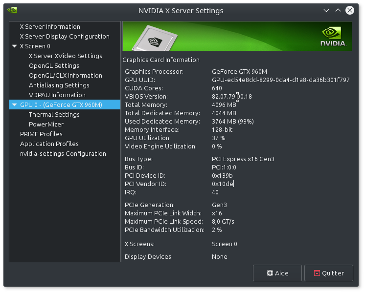
In this figure you see Nvidia GPUs, where the Nvidia settings panel is a handful to monitor the GPU memory and occupancy rate. After the loading of the whole MNIST dataset you see that 93% of the graphic memory is used.
If we change the shape of input vectors from (784, 1) to (28, 28), their raw memory size is the same because their support textures have the same number of texels ( 784*1 = 28*28 ). But this time the whole MNIST dataset occupies only around 280MB of the graphic memory, so more than 10 times less. Indeed, a one pixel wide texture like our (784, 1) input vectors is not stored efficiently because no texel has a complete 2D neighborhood. The memory occupied by the square textures is still above the theoretical value because the memory is paginated (or divided in blocks which are indivisible) and there are still edge effects since these textures are small.
To optimize GPU texture compression, we should:
- Use textures whose shape is as close to a square as possible.
- Group multiple textures into a few large textures, called texture atlas.
If we allocated only a few very large square textures, we would have little edge effects and few partially empty memory blocks. The actual occupied memory size will get closer to the theoretical value. To keep our implementation simple, we do not take account of these improvements and we always use textures which resolution is the same as the dimensions of the encoded matrix.
Feedforward
This is the sigmoid activation function declaration in network.js:
WGLMatrix.addFunction('y=1./(ONE+exp(-x));','ACTIVATION');
This is the feedforward part written in network.js:
self.feedforward=function(a){//Return the output of the network if ``a`` is input.for(vari=0,inp=a;i<self._nConnections;++i){//from input to output layer,// compute WI+B and store the result in _z:self.weights[i].fma(inp,self.biases[i],self._z[i]);//apply actFunc to _z and store result to _yself._z[i].apply('ACTIVATION',self._y[i]);//set input for the next iterationinp=self._y[i];}returninp;}
The first attempt
We have transcoded a MNIST classifier written in Python/Numpy to JavaScript/WGLMatrix. The code can be found in chapter3/5_MNIST. This example comes from Chapter 1 of Michael Nielsen’s online book, Neural networks and Deep learning. It is described on: http://neuralnetworksanddeeplearning.com/chap1.html. The neural network of the classifier is shallow. It has only three neuron layers:
- The input layer has 784 units (it takes 28x28 pixels digit images)
- There is 1 hidden layer with 30 neurons
- The output layer has 10 neurons (one per digit)
It is densely connected and the activation function is the sigmoid function. This network is trained over 30 epochs with eight samples per minibatch and a learning rate of 3.0 (per minibatch). There are 50000 samples in the training dataset and 10000 in the testing dataset. The best success rate on test data is 95.42% at epoch 27.
These are the benchmarks:
- Python/Numpy implementation (Python = 2.7.12, CPU = Intel Core i7-4720HQ): 318 seconds
- JavaScript/WebGL implementation (Chrome = 65, GPU = Nvidia GTX960M): 942 seconds
Note: matrix operations processed by Numpy are done by lower level linear algebra libraries like BLAS or LAPACK. They use the CPU very efficiently with linear algebra advanced features like SIMD instructions. They are much faster than if they were done by native Python functions.
This benchmark is not very good for our implementation. But we will surpass the Numpy implementation with a few improvements.
Improving the performance
You can test the improved version of learning on MNIST dataset on chapter3/6_MNISTimproved.
We do not use the RGBA channels at all in the previous implementation. Operations are uselessly duplicated over the four channels. We will use them separately in order to process four input vectors in parallel. This is doable because the size of a minibatch is a multiple of four (eight in the previous example). For testing data, we pack each four input/output vectors into one input/output vector by multiplexing over RGBA channels. The same execution time for our WebGL implementation drops from 942 seconds to 282 seconds. This is now better than Python/Numpy.
But the GPU utilization rate is only around 30% because textures encoding matrices are too small. Indeed, there is a bottleneck if we render to a texture which size is smaller than the number of GPU computing units: there is not enough work and some computing units stay idle.
So we need to render to larger textures. There are several solutions to overcome this problem:
- We can group several minibatch sample parameters in one texture. It consists in implementing texture spatial multiplexing as we have done RGBA multiplexing over minibatch samples. This solution speeds up learning, but it does not improve the network efficiency for exploiting.
- We can increase the number of neurons per layer. The core idea consists in adapting the neural network structure to the hardware architecture. We choose this solution.
We consider another network to learn the MNIST dataset:
- The input layer has 784 units (it takes 28x28 pixels digit images).
- There are two hidden layers with 256 and 64 neurons.
- The output layer has 10 neurons (one per digit).
We train it over 20 epochs with eight samples per minibatch with a learning rate of 1.0. Now the GPU works at 65% on average. Our implementation execution time is 344 seconds whereas the Python/Numpy implementation execution time is 1635 seconds (and the best success rate on test data is 96.45% at epoch 18). So our implementation is almost five times faster. We could still use the GPU more intensively, up to a 100% use rate, by increasing the hidden layers sizes. The performance ratio between our implementation and the Python one would climb higher. But we won’t get better results on test data because of overfitting problems (we should implement regularization or dropout algorithms to solve them, or implement convolutive connectivity).
With a low end GPU (the laptop used for benchmarks has also a low end Intel HD4600 GPU), the same learning takes 587 seconds. This is still almost three times faster than the CPU implementation.
Summary
We started this chapter by a minimal implementation of WebGL to draw two triangles to fill the viewport. The learning curve of WebGL is very steep at first and this is the most difficult part. WebGL appears as heavy plumbing where we need to write a lot of code and to create many different objects before rendering. But the more we practice it, the more it seems logical and well conceived. After the first rendering, the learning becomes incremental.
Then we use WebGL to compute in parallel pixel colors forming a beautiful Mandelbrot fractal. The rendering is fast despite each pixel require a quite heavy computation. Subsequently, we master this power to accelerate our calculations. We implement render to texture to get the result of a computation step to use it at a next step instead of directly displaying it. We implement our first WebGL simulation: the Conway game of life.
We tackle the floating-point computation problems. WebGL is designed for low precision computations because the RGB colors values do not need to be encoded with more than eight bits per component. So we need to consider several execution paths depending on hardware capabilities and WebGL version. We apply this new know-how to transform our previous simulation into a thermal diffusion simulation, dealing with physical continuous variable instead of discrete parameters.
We build our own linear algebra library, which can handle all standard floating-point values matrix operations. We put it to the test with the handwritten digit recognition using the MNIST dataset. Finally, we optimize the implementation to make it faster than the Python/Numpy equivalent.
This chapter is useful both to improve the existing WebGL implementations or to build a custom one. Whatever the software overlays used above WebGL, it is not possible to optimize correctly or to add functionalities efficiently without understanding the underlying mechanisms. It can also be a starting point toward the infinite world of real time hardware accelerated rendering.
In the next chapter we will look at how to extract data from the browser, such as loading image data from URLs, parsing the frames from the webcam, or parsing the data from the microphone.