
Chapter 1. Introduction to deep learning
This chapter is a gentle introduction to the main mathematical and practical concepts and architectures of deep learning. We focus on the mathematical concepts of supervised classification, which is a process of finding the correct class labels for unseen elements from a set of labeled training data. Once you understand the principles, you can apply the same techniques to other supervised tasks such as regression.
Note: All of the source code used in this book can be found here: https://github.com/backstopmedia/deep-learning-browser. And, you can access the demo of our Rock Paper Scissors game here: https://reiinakano.github.io/tfjs-rock-paper-scissors/. Also, you can access the demo of our text generation model here: https://reiinakano.github.io/tfjs-lstm-text-generation/.
We start the chapter with introducing the math behind neural networks. After reading this first section, you should be comfortable computing a pass through a simple pre-trained neural net for a binary classification task.
In the next section, we cover the techniques behind training the neural network based on labeled training data. After this section, you will understand the importance of loss functions, how the back-propagation algorithm works, and the differences between optimization techniques such as Gradient Descent and Nesterov Momentum.
In the third section, we discuss popular deep learning architectures such as AlexNet and ResNet. We also focus on very efficient layer structures that can run smoothly within the JavaScript engine of modern browsers, such as the Inception modules of GoogLeNet and the Fire modules of SqueezeNet.
The math behind deep neural networks
This first section gives an overview of the basic mathematical concepts behind neural network and deep learning. We focus mainly on computing the output of a deep neural network from an input data sample, which is often referred to as model inference.
Here we show that neural network inference consists mainly of a combination of multiple nested weighted linear functions, non-linear activation functions, and normalization. In a two-dimensional world the weighted linear function is a line equation. Activation functions are functions that activate as soon as the input value reaches a threshold. We refer to them as gates or non-linearities; normalization functions consist mainly of mean subtraction and division by standard deviation.
In a simplified classification task, the line equation describes the separation line between elements of two different classes. If the two classes are linearly separable, then the perfect classifier is a separation line with all elements of one class on each side. Inserting the coordinates of a point into the line equation returns a multiple of the signed distance to this line, where the sign represents the side of the line. The non-linear activation function transforms this signed distance to a different value. Popular transformations are, for example, returning the sign (+1 or -1) of the value, returning +1 or 0 or returning only positive values and 0 otherwise. You will see these activation functions and discuss their mathematical properties later. Normalization functions transform all points into a normalized space centered at 0 with a standard deviation of 1.
As you can see, these concepts are pretty intuitive and should be covered in most high school curricula. We will add a bit of complexity by operating in a n-dimensional space, instead of two dimensions, and nesting the functions to build a network.
The Perceptron - gated linear regression
The first advances toward a mathematical framework for artificial intelligence and machine learning were developed in 1958 by the psychologist F. Rosenblatt. He built a simplified mathematical model of a neural brain cell, the Perceptron, to mimic the biological learning behavior through activation and repetition.
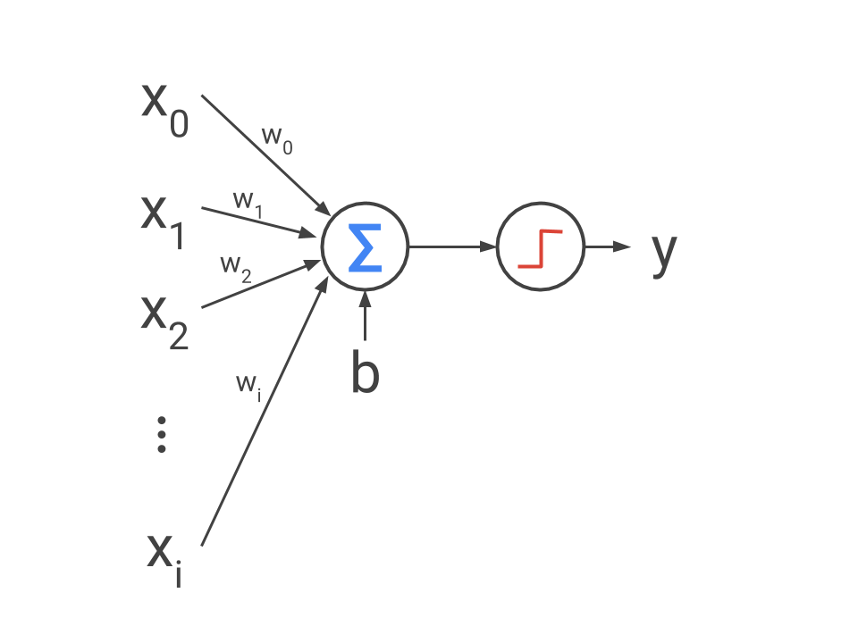
As you can see in this figure, the Perceptron computes a weighted sum of all input variables, x_i, and is followed by an activation gate represented by a step function. The gate fires (outputs 1) if the weighted sum of inputs is greater than 0. This is the Perceptron equation, which is a weighted sum of inputs wrapped by the step function.
![]()
In this section, we show that this simple mathematical operation written in the 50’s is the foundation of most of today’s deep neural network architectures. Moreover, we will explain that the mathematical concept of the Perceptron is very much the same for computing the output of a binary classification using a multi-dimensional line equation as a linear separation between two classes.
The line equation
Let’s start with a two-dimensional line equation.
![]()
In this case, k is the slope of the line and d the offset of the line from the center. Using the variables a, b and c instead of k and d (where k = -frac{a}{b} and d = -frac{w_0}{b}), you might have also seen a line representation like the following.
![]()
This equation has the nice property that inserting a point P = (p_1, p_2) into the line equation, the sign of the result represents on which side of line point P lies. This function hence characterizes a (trained) linear classifier that can separate data points into two classes, one for each side of the line.
![]()
The absolute value of the result is a multiple of the shortest distance d between the point and the line: d cdot sqrt{a^2 + b^2} = a cdot p_1 + b cdot p_2 + c. This value is also called class score.
When looking at the above example we see a striking similarity to the Perceptron equation with the only difference that the activation gate here is using the sign function. Imagine the point P is the two-dimensional of an element and the line is a two-d binary classification model, then y returns use the class +1 or -1. Finding the optimal separation line will be discussed in the second section of this chapter.
The Hyperplane Equation
As a next step, you can rewrite the line equation as a matrix representation, which is useful if you are dealing with more than two-dimensions.
![]()
The line equation is represented by a weight vector vec{w}^mathsf{T} = [ hinspace a hinspace b hinspace]. This equation can now be extended to an n-dimensional space using an n-dimensional weight vector vec{w} and input vec{x}. This multi-dimensional line equation is called a hyperplane.
Note: In machine learning, many problems are high-dimensional. One example is computer vision where deep learning models operate on pixel values. For a grayscale input image with the dimension 100 imes 100 the separating hyperplane would be defined in a 10000-dimensional space.
A linear binary classifier
Instead of using a simple step or sign function as a gate, we generalize the gate into an activation function h(x). The linear classifier equation now becomes the following, where the variable b now represents the bias instead of c in the two-dimensional case.
![]()
The above equation is the vector representation of the Perceptron equation with a generalized activation function. Hence, you can think of the Perceptron, also called Neuron, as a linear multi-dimensional binary classifier that separates data into two classes by using a linear hyperplane.
Let’s look at three different two-dimensional datasets with data points of two classes. The following figure shows these datasets, whereas the color of each dot represents the corresponding classes. Classifying this data would mean to draw a geometric shape that has all samples from the same class on one side and all other samples of the other class on the other side of the shape.
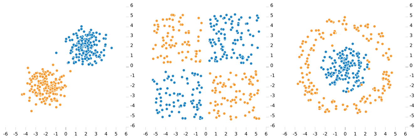
The Perceptron as a linear classifier has a huge intrinsic disadvantage: it can only correctly classify elements that are linearly separable; in 2D, the classify is a line. Hence, only the left dataset in the above figure can be divided into their distinct two classes using a single line. The XOR dataset can only be separated by using multiple combinations of line segments to separate and then to combine the diagonal counterparts. We will look into this problem in the subsequent section. The dataset on the right in the above figure requires a more sophisticated classifier to correctly label all data points.
The multi-layer Perceptron
One big drawback of the Perceptron is that it can only be used for linearly separable classes. The reason is that the Perceptron consists only of a weighted sum of inputs that can only represent a linear separation function. If you consider the XOR problem where both classes cannot be separated with a single line, you need to find a more flexible solution that can combine line segments for more complicated separations.
Let’s aggregate multiple neurons in one layer, such that each neuron generates an output y_i. Combine all neuron weights and biases of this layer into a weight matrix mathbf{W} and a bias vector vec{b}.
![]()
The above equation mathbf{W} vec{x} + vec{b} is often referred to as fully-connected layer. Hence, a fully-connected layer is defined by the number of neurons. It computes n outputs for n neurons, whereas each output is the result of the Perceptron equation.
The idea behind a multi-layer Perceptron is stacking multiples of these fully-connected layers together in which the output of every layer becomes the input of the following layer. Here is an example of stacking three layers together.
![]()
The multi-layer Perceptron is often referred to as hidden layers and represents a building block for most deep learning architectures. Multiple stacked fully-connected layers are called Artificial Neural Networks.
While models with multiple nested hidden layers can approximate arbitrary functions, they are much more difficult to train than a single fully-connected layer. Indeed, the combined error term of the network cannot be used to update the weights of the individual layers. In the second section of this chapter you will learn more about the back-propagation algorithm that splits the combined error into layer-wise errors, which makes the training of nested layers possible.
We recommend you try playground.tensorflow.org to fiddle with different input data, including activation functions and the number of neurons and hidden layers.
Convolution and pooling
Fully-connected layers come with a few disadvantages when working with two-dimensional image data. First, the number of trainable parameters (all entries in W and vec{b}) is quite large. A single layer of 1024 neurons for a vectorized 100 imes 100 RGB image already has 1024 imes 100 imes 100 imes3 (parameters of W) + 1024 (parameters of vec{b}) trainable parameters. Moreover, the local neighborhoods of pixel values are treated independent of each other and every input pixel is related with each other in every neuron.
Sharing weights through convolution
A more efficient way for two-dimensional image data is to use a small two-dimensional n imes n local filter. For every output pixel, you compute the weighted sum of all n input pixels where the weights are the parameters of the filter. Do this by sliding the filter through all possible locations in an image and use the same filter weights for each location. This technique is called convolution, and is used also for classical image filters in traditional computer vision applications, such as with edge and blob detectors.
The convolution operation is described by the filter dimensions and two additional parameters: stride and padding. Stride and padding control how the filter (also called kernel) slides through the image locations. The stride parameter is the number of pixels that the filter is moved from one location to the next. If you slide a 3 imes 3 filter over a 100 imes 100 input image with a stride of 1 pixel, then the resulting output image will have a dimension of 98 imes 98 (you lose one pixel at each image border). Using stride 2, the output dimension would be halved. The padding parameter describes the number of additional constant pixel values (usually with the value 0) that are added around the input image, allowing you to control the output dimensions of a convolution. So, a 3 imes 3 filter with stride 1 and padding 1 will return the same output dimensions of the input image.
Many deep learning frameworks replace the numerical value of padding with the options same and valid. The reason for this is that depending on the filter dimension and stride, you have to manually compute the correct padding for keeping the output dimensions the same, or generating a valid output image. Using the same and valid options, the corresponding numerical padding value can be set automatically, which is much easier for the user.
Convolutional Neural Networks (CNNs) are neural networks that use convolution operators on two-dimensional image data. In contrast to ANNs where the input image pixels are simply stacked into a vector, in CNNs the input consists of a three-dimensional input volume of width, height, and depth (for RGB the color channels). In most networks, all input images of one batch are stacked into a fourth batch of dimensions, however, the image filters are applied to every volume of the batch.
A 2D Convolution Layer (also called Conv Layer) consists of a set of 2D filters. Each 2D filter is convolved along the spatial dimension per input depth dimension, and then computes a weighted sum over all depth dimension. So, one 2D filter creates one 2D output image for the whole input volume. By stacking multiple 2D filters along the depth dimension, we create multiple output images stacked along the depth dimension.
Due to weight sharing, Conv layers are much more efficient than fully-connected layers and can take advantage of local dependencies of two-dimensional data. In images these local neighborhoods are represented as multiple correlated neighboring pixels of the same shape, object, texture, etc. A Conv layer has w imes h imes d imes f + f number of parameters that need to be learned during training. The parameters w and h represent width and height of the filter, d represents the depth of the filter, and f the number of filters.
Similar to fully-connected layers, Conv layers are usually followed by a non-linear activation function. You will read more about activation functions in a later section of this chapter.
Reducing spatial dimensions through pooling
Using only Conv layers, it is possible, but very difficult, to control the spatial dimensions of the output volumes. In addition, Conv layers always contain trainable parameters. Pooling is a parameterizable subsampling operation that reduces the spatial dimension of the input data. If you have a background in computer vision, you may have seen this operation used in popular image filters such as Gaussian and Laplacian image pyramids: SIFT and SURF.
One of the non-trainable parameters of the pooling operation is the subsampling function used for the aggregation, where max and avg are the two most popular choices. Within a network, mostly max pooling is used due to the very simple gradient computation (more in the second section of this chapter). For n imes n pooling, these aggregation functions are applied to every n input pixels to create 1 output pixel. Similar to convolution, the pooling operation is also applied to all image locations using stride and padding parameters.
Activation functions
Non-linear activation functions transform the weighted sum of the hyperplane equation and image filters into an activated signal, so they only contain output values if they are greater than 0. These functions play an important role in neural networks, because they enable the stacking of layers. Without activation functions, the nested Multi-Layer Perceptron could be rewritten as a single layer equation, because it would consist only of weighted sums.
Activation functions are also organized in layers and embedded into the neural network architecture. They are usually inserted after every Conv and fully-connected layer. Within the network, ReLU and ELU activations are popular choices for threshold activations.
Some activation layers play a special role as an output for neural networks due to their mathematical properties and so are used as the last layer of a network. For example, the Softmax activation, which returns a vector whose values sum up to 1, which is a handful property for creating a classifier output.
In this section we will take a look at the most popular activation functions and their mathematical properties.
Sigmoid and hyperbolic tangent
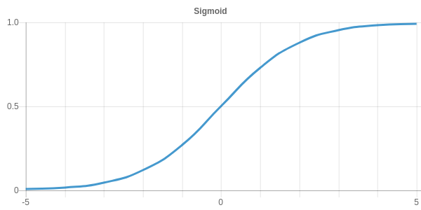
After the step function in the Perceptron equation, the sigmoid function was the most popular choice as an activation function in the 80’s. The reason for this is that the sigmoid function smoothly maps any value to a range of 0 and 1 and is continuously differentiable in contrast to the step function.
The sigmoid activation function is defined by the following equation.
![]()
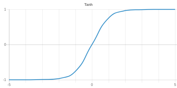
The second activation function heavily used in the 80’s was the hyperbolic tangent tanh. It has a shape quite similar to sigmoid with a value range of -1 and 1. Tanh was used because the numerical computation of tanh is much more stable. Numerical stability was and still is quite an important property of activation functions to avoid exploding gradients during training.
The tanh activation function is defined by the following equation.
![]()
ReLU, Leaky ReLU and ELU
Rectified Linear Unit (ReLU) is the most widely used non-linearity for deep neural networks. While not being differentiable at position 0, the ReLU function greatly improves the learning process of the network due to the fact that the total gradient is simply passed to the input layer when the gate triggers.
The ReLU activation function is defined by following equation.
![]()
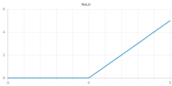
One of the problems of ReLU is that the activation of negative values is always 0. This problem is quite intuitive if you imagine a situation where all training samples are on the wrong side of the separation hyperplane. This situation would lead to an activation of 0 for every neuron resulting in an output of 0 and a loss of 0. With a loss of 0, we are never able to tune the weights of this neuron.
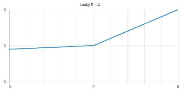
The Leaky ReLU or Parametric Leaky ReLU introduces a negative slope, ensuring that the activation for negative values is unequal 0. The slope can be tuned with the parameter a and is 0.01 for the standard Leaky ReLU.
![]()
Another problem of ReLU and Leaky ReLU is that both activation functions are not differentiable at 0. The Exponential Linear Unit (ELU) fixes this problem by approximating the Leaky ReLU function by a fully differentiable exponential function.
![]()

Softmax
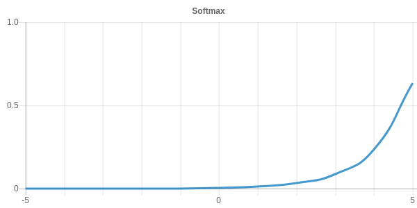
The softmax function normalizes all values to a range between 0 and 1 such that the sum of all values is equal to 1. It is defined by the following equation.
![]()
The softmax activation is commonly used in classification networks as the final output layer because it converts raw class scores into class probabilities. The resulting vector describes a probability distribution of the inputs.
Training deep neural networks
In the previous section we assumed that there is a way to compute the weights W such that the neural network represents the line (or hyperplane) that perfectly separates the elements of two (or multiple) classes. In this section, you will learn the concepts for training a neural network to find those weights W by using a set of labeled training data.
Given a set of training samples belonging exclusively to one class, you first need to compute how good the current hyperplane separates those samples into the distinct classes. Good always means that a certain error, such as the number of misclassified samples, or samples that are on the wrong side of the separation plane, are minimized. This function is called the loss function and evaluates the current fit of the classifier. You will see how the shape of the loss function can strongly affect the training and learning progress.
Once you have the combined loss of the classifier, it is not possible to start tuning the weights of the single nested layers in order to improve the overall model performance because each layer adds its individual contribution to the overall loss. This is the reason why neural networks didn’t become more popular in the 60’s. In order to properly tune the model weights, first you need to compute the contribution of each nested layer to the combined loss, a process called back-propagation. Once you know the loss per layer, tune the weights of each layer independently. This process requires you to compute the derivative of each layer. This is the reason why deep learning is often also referred to as differentiable programming.
Tuning the independent layer weights is done in an iterative stepwise approach. At each iteration step, the layer weights are adjusted in the direction of the negative gradient in order to optimize the loss function. A popular technique to do this is called Gradient Descent, however we will look also at more efficient techniques such as Nesterov Momentum and Adam.
The importance of the loss function
The most important ingredient for optimizing or training a model is a function evaluating how well that model represents the given training data, which we call the loss function. When defining it, aim for nice mathematical properties such as differentiability. When setting the derivative of a function to 0 you obtain the extreme of this function. In the case of training a neural network, the goal is to find the minimum of the loss function.
In the case of deep learning, the loss function is a very high (usually million) dimensional function, depending on all trainable network parameters.
The choice of a loss function depends on the task that should be performed with the model. Models for regression and classification with ordinal class labels can, for example, benefit from a loss function, taking into account the difference between the predicted value to the true value. Classifications with categorical classes, however, use only the true or false binary results.
In classification, a common loss function is the Cross-Entropy, which computes the fit of two probability distributions: the true probability of the ground-truth and the predicted probability distribution. It is often used in combination with the softmax activation. In regression, a common loss function is the sum of squared errors, the so called Mean Squared Error.
Regularization
A common problem of training models with thousands to millions of parameters is overfitting. The network learns the specific samples of the dataset instead of generalizing concepts. It can be diagnosed by comparing the success rate on training data to the success rate on test data: the network is good at predicting the correct classes for training data, but fails with predicting unseen data. One popular strategy to avoid overfitting is to add a regularization term to the loss function. The regularization term is computed by summing up the norm (mostly L1 and L2) of all trainable parameters of each layer.
The L1 regularization penalizes parameters different from 0 and pushes the weights to be sparse. L2 regularization penalizes large parameters and results in small parameters. L2 weight regularization is also called emph{weight decay} because the weights are shrunk before each update in the gradient descent.
The full training loss is mostly constructed by a classification or regression loss plus an additional regularization loss to improve generalization.
The back-propagation algorithm
Once you know the loss of your network prediction, you cannot unfortunately use this loss directly to update the weights of each individual layer. To do so, you first need to compute the amount of loss contributed by each layer and then tune the layer weights according to the gradient of the loss. You can find this gradient for each layer by iteratively stepping backwards through the network and applying the chain rule of differentiation to compute the gradient contribution for each layer. This algorithm is called Back-Propagation.
The chain rule is written as the following:
![]()
The meaning of the above equation is that instead of computing the changes of z based on x, you can compute the changes on z based on y multiplied by the changes of y based on x. If you translate this into a deep learning setting, you can say: Instead of computing the changes of the loss based on the model input, you can compute the changes of the network loss based on the output of the last layer, the loss of the last layer based on the output of the previous layer, etc. This technique let’s you separately tune each layer’s weights.
Optimization methods
To train a deep neural networks efficiently, you need an optimization algorithm that tunes the network weights in such a way that the classifier’s training loss decreases each training epoch. The classical is the most popular choice for this optimization when knowing the derivatives of the model use Gradient Descent (GD).
For GD first compute the gradient of the loss for each layer using back-propagation starting from the loss of the complete network. This gradient is a high-dimensional vector that points into the (negative) direction of the smallest loss. In a second step, update the weights by adding a multiple of the gradient to the weights. The factor to multiply the gradient is called the learning rate, and defines the step-size in which you are moving through the loss function’s space.
The following equation shows the update logic of the weights W_i of a layer i using gradient descent optimization, where alpha is the learning rate and L_i is the loss of a layer i.
![]()
In deep learning we use mostly mini-batch gradient descent, which incorporates benefits from both stochastic gradient descent using only one sample at a time, and a classical gradient descent using all samples at a time.
Due to the simplicity of GD, it also has a few disadvantages, such as fixed step size, problems with local minima, time of convergence, convergence with complicated loss functions, and more. Therefore, more robust techniques have been developed on top of gradient descent, such as Momentum, Nesterov Momentum, Adam, RMSProp, etc. You can pick up most of these algorithms and many more under the name Optimizer from most of the popular deep learning frameworks.
One way to improve the convergence of GD, is to use some sort of moving average of decaying gradients to build a velocity v for the GD update step. This algorithm is called Momentum and converges much faster than GD. The update step can be written as:
![]()
If you know the current momentum you can compute the gradient at the new position W + v instead of W. This variation is called Nesterov Momentum.
Summary
Now that we have the main mathematical and practical concepts and architectures of deep learning under our belt, we can move on to neural network architectures in the next chapter.