Chapter 4

Reliability Models

Louis J. Gullo

Introduction

Models are developed to simulate actual behavior or performance and to reflect or predict reality. A modeling methodology is needed to fully understand what models are and how they are useful. Maier and Rechtin [1, p. 11] state: “Modeling is the creation of abstractions or representations of the system to predict and analyze performance, costs, schedules, and risks, and to provide guidelines for systems research, development, design, manufacture, and management. Modeling is the centerpiece of systems architecting—a mechanism of communication to clients and builders, of design management with engineers and designers, of maintaining system integrity with project management, and of learning for the architect, personally.”

The goal of a reliability model is to set expectations on performance and reliability, and to represent reality accurately as closely as possible for the purpose of predicting or assessing future performance and reliability. A key focus in developing models is to ensure that no mission-aborting (mission-critical) component will fail during a required mission time. This focus could be extrapolated into no mission failures during the expected lifetime (over a number of missions). This goal is accomplished by identifying design weaknesses using experimental design modeling, analysis, and testing, to improve design for reliability such that mission interruptions are minimized or reduced over the anticipated life, and to reduce unscheduled downtime and increase system availability.

There are many times during a system or product life cycle when reliability modeling has value. First, in the system or product concept and development phase, modeling is valuable to help system architects and product designers to decide where and how much redundancy and fault tolerance is needed to achieve life-cycle requirements. Modeling may also be employed after initial development when a major redesign is being considered for product feature enhancements and technology refresh. If organizations want to continue using the systems beyond the expected life, they should conduct risk analysis with the aid of reliability models to compare the reliability of the design with the maintenance cost to refurbish. Reliability modeling helps organizations make the decision to determine when it is not economically feasible to support a system or refurbish a system beyond its expected lifetime.

One type of reliability model is the reliability prediction model. Reliability prediction models may be physics-of-failure (PoF) models, failure rate models, or mean-time-between-failures (MTBF) models. Reliability prediction models may take the form of probability density functions or cumulative density functions. Reliability prediction models may be useful for comparing the reliability of two different designs. A common approach for comparing the reliability of different design options is described in MIL-HDBK-217 [2], the military handbook for the reliability prediction of electronic equipment. The purpose of MIL-HDBK-217 is to establish and maintain consistent and uniform methods for estimating the inherent reliability (i.e., the reliability of a mature design) of military electronic equipment and systems. It provides a common basis for reliability predictions during acquisition programs for military electronic systems and equipment. The handbook is intended to be used as a tool to increase the reliability of the equipment being designed. It also establishes a common basis for comparing and evaluating reliability predictions of related or competitive designs. The military handbook includes component failure rate models for various electronic part types. A typical part stress failure rate model is shown in this example. The part stress failure rate, λ_p, for fixed resistors is

(1)

where

π_b = base failure rate (a function of temperature and stress)

π_E = environmental factor

π_R = resistance factor

π_Q = quality factor

Reliability models may be created to predict reliability from design parameters, as is the case when using MIL-HDBK-217, or they may be created to predict reliability from experimental data, test data, or field performance failure data. One type of reliability model, which is developed based on design parameters, is called a defect density model. These types of reliability models have been used extensively for software reliability analysis. Various types of software reliability models are provided in IEEE 1633–2008 [3], a practice recommended for software reliability engineering. Software reliability models are based on design parameters, the maturity of a design organization's processes, and software code characteristics, such as lines of code, nesting of loops, external references, flow in and flow out, and inputs and outputs, to estimate the number of defects in software. Reliability models statistically correlate defect detection data with known functions or distributions, such as an exponential probability distribution function. If the data correlate with the known distributions, these distributions or functions can be used to predict future behavior. This does not mean that the data correlate exactly with the known functions but, rather, that there are patterns that will surface. The similarity modeling method, discussed later in the chapter, estimates the reliability of a new product design based on the reliability of predecessor product designs, with an assessment of the characteristic differences between the new design and the predecessor designs. This is possible only when the previous product designs are sufficiently similar to the new design and there is sufficient high-quality data. The use of actual performance data from test or field operation enables reliability predictions to be refined and “measurements” to be taken. The higher the frequency and duration of the correlation patterns, the better the correlation. Repeatability of patterns that exist will determine a high level of confidence and accuracy in the model. Even with a high level of confidence and good data correlation, there will be errors in models, yet the models are still useful.

George Box is credited with the saying: “All models are wrong, some are useful.” Box is best known for the book Statistics for Experimenters: Design, Innovation and Discovery [4], which he coauthored with J. S. Hunter and W. G. Hunter. This book is a highly recommended resource in the field of experimental statistics and is considered essential for work in experimental design and analysis. Box also co-wrote the book Time Series Analysis: Forecasting and Control [5] with G. M. Jenkins and G. Reinsel. This book is a practical guide dealing with stochastic (statistical) models for time series and their use in several applications, such as forecasting (predicting), model specifications, transfer function modeling of dynamic relationships, and process controls, to name just a few applications. Box served as a chemist in the British Army Engineers during World War II, and following the war, received a degree in mathematics and statistics from University College London. As a chemist trying to develop defenses against chemical weapons in wartime England, Box needed to analyze data from experiments. Based on this initial work and his continuing studies and efforts thereafter, Box became one of the leading communicators of statistical theory.

As a co-developer of PRISM (a registered trademark of Alion Science and Technology) along with Bill Denson from the Reliability Analysis Center, Samuel Keene believed (in the 1990s) that the underlying thesis in this reliability model was that the majority of significant failures tie back into the process capability of the developing organization. He worked in the MIL-HDK-217 working group during that time. He completed his work with a view that parts are the underlying causes of system failures. Then to his surprise he found that 95% of the problems on production systems were traceable to a few parts experiencing a specific cause failure, with the majority of failures related to system-level causes not related to the inherent reliability of the parts.

Many types of reliability models are described in this chapter. Reliability models are developed for systems, hardware, and software to develop optimized solutions to reliability problems. System reliability models may be classified as repairable models or non-repairable models. An excellent reference for probabilistic modeling of repairable systems is by Ascher and Feingold [11]. An overview of models and methods for solving reliability optimization problems since 1970's is presented by Kuo and Prasad [12]. A common form of system reliability models is a Reliability Block Diagram (RBD).

Reliability Block Diagram: System Modeling

System reliability block diagrams (RBDs) and models start with reliability allocations derived and decomposed from requirements. These allocations are apportioned to the blocks of the model. The model is updated with reliability predictions based on engineering analysis of the design to validate the model initially. The predictions are updated with actual test and field reliability data to validate the model further.

What is an RBD?

• An RBD is a logical flow of inputs and outputs required for a particular function.
• There are three types of RDB diagrams:
  • Series RDB
  • Parallel RBD (includes active redundancy, standby, or passive redundancy)
  • Series–parallel RBD

Examples of each RDB type are shown later in the chapter.

Two of the most frequently used RDB models are basic reliability models and mission reliability models. These two types of RBM models are discussed in detail in MIL-STD-756B [6] and by O'Connor [7]. The basic reliability model may be in the form of a series RBD model. A basic reliability model is a static model that demonstrates how to determine the cost of spares provisioning to support the maintenance concept throughout the life cycle. The basic reliability model is a serial model that accumulates the failure rates of all components of a system. This type of model considers the inherent failure rate of each hardware or software component or module. It helps the analyst recognize the fact that adding more hardware or software to a system decreases the reliability of the system and increases the cost to maintain the system.

The mission reliability model is another static model that demonstrates the system reliability advantages when using a fault-tolerant design that includes redundancy and hot sparing concepts to meet mission reliability requirements. A mission reliability model may be in the form of a parallel or a series–parallel RBD. The mission reliability requirement may be stated in terms of the probability of a mission-critical failure during the mission time. Mission time may be the time it takes to drive from point A to point B, or the time it takes for a missile to reach its target. The mission reliability model could be a combined serial–parallel RBD model which recognizes that adding more hardware or software does not necessarily decrease the reliability of the system, but increases the cost to maintain the system. In many cases for a parallel RBD model, adding redundant hardware will increase the reliability of the system and increase the maintenance costs during normal operation. The increase in maintenance cost results from the additional hardware to remove and replace in the system when a system failure occurs, from more spare hardware to store and replenish, and from higher logistics times to transport and supply the spares and perform the maintenance tasks.

Example of System Reliability Models Using RBDs

• The reliability of a complex system depends on the reliability of its parts.
• A mathematical relationship exists between the parts' reliability and the system's reliability.
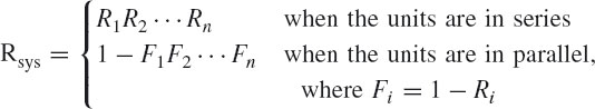
• If a system consists of n units, with reliability R_i for unit i, then in simple terms, the system reliability, R_sys, is given by

  

Case 1

A series RBD model (Figure 1) consists of four components, A to D, each with a reliability of 0.99 for the conditions stated and time t. The four components are connected in series and an equation is written to show the mathematical expression for this model:

(2)

In this case, a series reliability model results in a total system reliability that is less than the reliability of a single component.

Case 2

A parallel RBD model (Figure 2) consists of three components, A to C, that are connected in active parallel with each component's R_i = 0.99. An equation also shows the mathematical expression for this model:

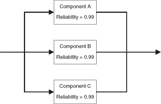
(3)

where F_i = 1 − R_i and R_i = 0.99. In this case, a parallel reliability model results in a total system reliability that is greater than the reliability of each of the components.

Case 3

A series–parallel RBD model (Figure 3) consists of five components, A to E, that are connected in an active series–parallel network with each component's R_i = 0.99. An equation shows the mathematical expression for this model:

(4)

where F_i = 1 − R_i and R_i = 0.99. In this case, a series–parallel reliability model results in a total system reliability that is greater than the reliability of any one component.

System Combined

• If the specified operating time, t, is made up of different time intervals (operating conditions), t_a, t_b, t_c, etc.:

• The system combined reliability is shown in equation (5) and is simplified in equation (6):

(5)

(6)

Note: In this example, where the reliability distribution is an exponentia distribution, the assumption is made that the failure rate is constant over time.

Reliability Growth Model

“Other types of reliability models are reliability growth models such as the Duane growth model or the Crow AMSAA model. Reliability growth modeling is a dynamic modeling method to demonstrate how reliability changes over time as designs are improved. Reliability growth is useful when there is a Test Analyze and Fix (TAAF) program to discover design flaws and implement fixes [11]. Reliability growth curves are developed to show the results of design improvements as demonstrated in a growth test, whenever the interarrival times tend to become larger for any reason. Other reliability growth models available in the literature include the Nonhomogeneous Poisson Process (NHPP) models, including the Power Law model, Cox-Lewis (Cozzolino) model, McWilliams model, Braun-Paine model, Singpurwalla model, Gompertz, Lloyd-Lipow, and logistic reliability growth models [8,11]. A reliability growth model is not an RBD model. Reliability growth models are designed to show continuous design reliability improvements. Reliability growth models assess the rate of change in reliability over time, which can be used to show additional improvements beyond a single RBD model.”

Similarity Analysis and Categories of a Physical Model

Reliability modeling using similarity analysis is discussed in refs. [6, 9, 10]. The similarity analysis method should define physical model categories to compare new and predecessor end items or assemblies. These categories are shown in Table 1. The first five categories are part-type component-level categories that quantify the field failures due to component failure and may be partitioned to various levels of detail. The next two categories are design and manufacturing processes. Additional categories may be added for equipment-specific items not related to part type or process categories.

Table 1 Example of Physical Model Categories

In this example, failure causes are divided into physical model categories. Categories 1 to 5 are for failures in service due to component failure; the next two categories are for processes (design and manufacturing) that can be controlled by the end item supplier, and additional categories (categories 8 and higher) can be added for product-specific items. Manufacturing-induced component failures are categorized under manufacturing processes (category 6), and misapplication and overstress are categorized under the design processes (category 7).

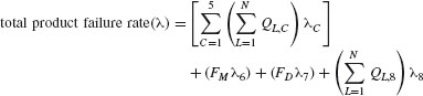
Equation (7) is used to calculate the total product failure rate and the projected mean time between failures (MTBF). The total product failure rate is computed by summing the failure rates for categories 1 through 8. Projected MTBF is computed by taking the inverse of the total product failure rate:

(7)

where

Q_L,C = part quantities for line replaceable unit (LRU), assembly L, and physical model category C

L = one LRU or field-replaceable unit (FRU)

C = one physical model part-type component-level category (categories 1 to 5)

N = total number of LRU, assembly, or functional levels in the assessment.

λ_C = expected category failure rate for physical model category C

F_M = process factor for the manufacturing process failures in category 6

F_D = process factor for the design process failures in category 7

λ₆ = expected category failure rate for the manufacturing process—physical model category 6

λ₇ = expected category failure rate for the design process—physical model category 7

λ₈ = expected category failure rate for physical model category 8

Formula representation (7) assumes one user-defined physical model category (category 8). If additional user-defined categories are required (e.g., category 9, 10, etc.), they will be treated in the same manner as category 8.

Companies must understand the inherent design reliability of complex systems where RDBs and similarity analysis methods are not adequate. To compute the reliability of complex systems, companies may use Monte Carlo simulations and models included with RDBs, and Markov chains and models to supplement RDBs.

Monte Carlo Models

Monte Carlo models and simulations provide a means to assess future uncertainty for complex physical and mathematical systems. They are often applied to RBDs in the development of reliability models for complex systems. Monte Carlo analyses produce outcome ranges based on probability, incorporating future uncertainty. Monte Carlo methods combine analysis of actual historical data over a sufficient period of time (e.g., one year) with analysis of a large number of hypothetical histories (e.g., 5000 to 10,000 iterations) for a projected period of time into the future. These models rely on repeated random sampling to compute reliability. These methods are useful when it is infeasible or extremely difficult to compute an exact result with a deterministic algorithm. Monte Carlo methods are used in mathematics, such as for the evaluation of multidimensional integrals with complicated boundary conditions and in reliability analyses to correlate electrical and environmental stresses to time-to-failure data. Variation in failure rates could be analyzed based on multivariant stress conditions, such as high electrical stress with high-thermal-stress conditions, high electrical stress with low-thermal-stress conditions, and low electrical stress with low-thermal-stress conditions. These types of Monte Carlo analyses may also be known as four- or five-corner analyses, depending on the number of stress parameters that are evaluated simultaneously.

Markov Models

For systems subject to the dynamic behavior of functional dependence, sequence dependence, priorities of fault events, and cold spares, Markov models and Markov chain methods are used for reliability modeling. Markov chain methods consider each component failure, one by one. Markov models are very useful for understanding the behavior of simple systems, but as the system becomes more complex, there is a major drawback. As the number of states increase significantly, the number of probabilities to be calculated increases, so that the Markov method becomes very cumbersome compared to RDB models.

Consider a simple system with one component in service and one spare component in stock. There are three possible states:

• State 1: both components serviceable, one component in service and one component in supply
• State 2: one component serviceable, one component unserviceable and in repair
• State 3: both components unserviceable

For any given time interval, the system may remain in one state or change state once, twice, or more times, depending on the length of time chosen. If we consider a time interval where the system is initially in state 1, all the possibilities can be shown diagrammatically as in Figure 4.

Typical inputs and outputs from a Markov model are:

State = system state

λ = failure rate

μ = repair rate

P = probability

P_ii = probability of system remaining in state i

P_ij = probability of system changing state from state i to state j

Further explanation of Monte Carlo methods, Markov methods, and reliability prediction models may be found in IEEE 1413.1 [10].

Modeling a system is consistent with the design for reliability (DFR) knowledge thread of the book: that modeling a system that includes DFR eliminates the potential for mission-aborting failures. Electronic designs will have random isolated incidences that will not warrant design changes, such as failures within a six sigma defect envelope: for example, 4,000,000 devices tested and one integrated circuit (IC) component fails because of a broken bond wire that was tested previously. These defects may result in system-degraded performance but not mission-critical failures. Modeling a system that allows for scheduled or preventive maintenance or condition-based maintenance is to develop views and viewpoints that incorporate an understaning of what components of the system warrant replacement and provide for an allowable failure rate while the system is performing its mission. More details are available in the references.

Reliability models which assume that a system failure model is merely the sum of its parts failure rates are inaccurate, yet these methods exist today. Electronic part failures account for 20 to 50% of total system failures. For nonelectronic parts, the failure distribution percentage is even smaller. The majority of the failure distribution is related to customer-use or customer-misuse conditions or defects in the system requirements. The reason that parts are usually blamed for many, if not all, failures is because it is easy to allocate failures to part numbers in showing proof of root-cause analysis and drilling down to determine the physics of failure. As we see it, the problem is not the part but the use of the part or out-of-spec conditions that caused the failure.

In a good failure reporting, analysis, and corrective action system (FRACAS), actual performance data from testing and field experience is useful to modify or update the reliability models and improve confidence in the models. Failure cause codes will be created for such failure causes as design failures, design process failures, customer-induced failures, manufacturing process and workmanship defects, supplier process defects, and supplier part design failures, as a minimum. These failure-cause categories are used to revise reliability models and build the model accuracy. All these failure causes should be correctly coded in the FRACAS database and correlated with their appropriate failure-cause categories which are applied in the models (discussed earlier). For example, a failure caused by the electrical assembly designer's misapplication of a part in a circuit causing electrical overstress should be coded as a design-related failure and not as a supplier part issue. Care must be taken during root-cause failure analysis to determine the exact failure mechanisms and attribute failure causes to the proper cause codes for future modeling and data analysis. For an effective useful model, all the causes of system failures should be allocated a failure rate. The early development models should be improved constantly using all available data collected from testing and field performance. With the improvements made to the model using FRACAS data and other sources of statistical data, the model increases in accuracy and usefulness. In the context of George Box's quote, “All models are wrong, some are useful,” as statistical data are added to a model, its usefulness increases and becomes more correct, or less wrong and more useful.

References

[1] Maier, M. W., and Rechtin, E., The Art of Systems Architecting, 2nd ed., CRC Press, Boca Raton, FL, 2002.

[2] Military Handbook for the Reliability Prediction of Electronic Equipment, MIL-HDBK-217, Revision F, Notice 2, U.S. Department of Defense, Washington, DC, Feb. 1995.

[3] Recommended Practice on Software Reliability, IEEE 1633–2008, IEEE, Piscataway, NJ, June 2008.

[4] Box, G., Hunter, J., and Hunter, W., Statistics for Experimenters: Design, Innovation and Discovery, 2nd ed., Wiley-Interscience, Hoboken, NJ, 2005.

[5] Box, G., Jenkins, G. M., and Reinsel, G., Time Series Analysis: Forecasting and Control, 4th ed., Wiley, Hoboken, NJ, 2008.

[6] Military Standard on Reliability Modeling and Prediction, MIL-STD-756B, U.S. Department of Defense, Washington, DC, 1981.

[7] O'Connor, P., Practical Reliability Engineering, 4th Ed., Wiley, Hoboken, NJ, 2002.

[8] Kececioglu, B. D., Reliability Engineering Handbook, Vols. 1 and 2, 2nd ed., Prentice Hall, Upper Saddle River, NJ, 1991.

[9] Johnson, B., and Gullo, L., Improvements in reliability assessment and prediction methodology, presented at the Annual Reliability and Maintainability Symposium, 2000.

[10] IEEE Guide for Selecting and Using Reliability Predictions, IEEE 1413.1–2002 (based on IEEE 1413), IEEE, Piscataway, NJ.

[11] Ascher, H., and Feingold, H., Repairable Systems: Modeling, Inference, Misconceptions and Their Causes, Marcel Dekker, New York, 1984.

[12] Kuo, W., and Prasad, V. R., An annotated overview of system-reliability optimization, IEEE Trans. Reliab., vol. 49, no. 2, 2000, pp. 176–187.