Chapter 5: Networking in Motion

In the previous chapter, we talked in depth about the hardware and the operating system. Any trading system must collect data from the exchange and make decisions based on this data. To do so, communication will be essential in the performance of the high-frequency training (HFT) system. In this chapter, we will review how trading systems communicate in depth, how to use networks in HFT systems, and how to monitor network latency.

In this chapter, we will cover the following topics:

• Understanding networking in HFT systems
• Network communications between systems in HFT
• Important protocol concepts
• Designing financial protocols for HFT exchanges
• Interior networks versus exterior networks
• Understanding the packet life cycle
• Monitoring the network
• Valuing time distribution

The following section will describe networking basics; we will go through the fundamentals that we will optimize later on.

Understanding networking in HFT systems

Trading systems receive market data and send orders from/to exchanges. The numerous processes spread out across different machines within a trading system need to communicate with one another—for instance, a process keeping track of a position of an instrument across the design will need to send information to all components regarding the position of a given asset. Networking defines how devices are interconnected with each other. Networking is required to transfer data from a machine to another one (by extension, to an exchange).

The network is the underpinning of all HFT systems and needs to be considered as carefully as the design decisions for software systems.

The device ensuring communication in any system is called the Network Interface Card (NIC). It allows communication between the computer where software runs and the outside world. When we understand how a trading system works, we must examine the layered model used to describe the networking stack within the operating system required for computers to talk with each other.

Learning about network conceptual models

The Open Systems Interconnection (OSI) model is arguably the most common depiction of how computers speak to each other in modern networked environments. The OSI model is a conceptual framework used to describe the functions of a networking system. The following screenshot depicts the complete seven layers of the OSI model and the related operations typically found at each layer:

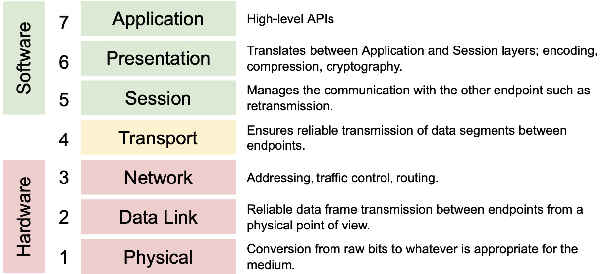
Figure 5.1 – The seven-layer OSI model

This model is divided into seven independent layers, which all have specific functions and communicate with their adjacent layers only and don't communicate with all the other layers. The layers are described in more detail here:

• The session, presentation, and application layers: These three layers can be regrouped (to simplify) because these are the layers that we will use at the software level. In HFTs, we focus on the following four layers because they give advanced optimization opportunities.
• Transport layer: This manages the delivery and also contains errors in data packets. Sequencing, packet size, and transfer of data between systems are the responsibility of the network layer. In finance, we mainly use two protocols: the Transmission Control Protocol (TCP) and the User Datagram Protocol (UDP).
• Network layer: This receives frames from the data link layer and delivers them to the intended destinations using logical addresses. We will use the addressing protocol called Internet Protocol (IP). Unlike IP version 6 (IPv6), IP version 4 (IPv4) is a light and user-friendly protocol and is the most widely used protocol in the financial sector.
• Data link layer: This layer corrects errors that may have occurred at the physical layer by detecting errors with techniques such as parity checks or cyclic redundancy checks (CRCs).
• Physical layer: This is the media that two machines use to communicate, including optical fiber, copper cable, and satellite. All these media have different characteristics (latency, bandwidth, and attenuations). Based on the type of application we want to build we will leverage one versus the other. This physical layer is considered the lowest layer of the OSI model. It is concerned with delivering raw unstructured data bits across the network, either electrically or optically, from the sender's physical layer to the receiver's physical layer. Network hubs, cabling, repeaters, network adapters, and modems are examples of physical resources found at the physical layer.

As you can see from how the layers are grouped in Figure 5.2, we often refer to several of them simultaneously. For example, we may refer to layers 5-7 as the software layer and layers 1-3 as the hardware layer, with layer 4 getting mixed between the two. This is so common that a simplified model that consolidates the software, transport, and hardware layers is frequently used and looks like this:

Figure 5.2 – Simplified OSI model

Now that we have discussed the high-level layered path that a packet must take when moving through the networking stacks on two communicating computers, we will discuss how to design a network for HFTs.

Network communications between systems in HFT

When designers build a network for HFT systems, they focus on the different modes of communication. Because microseconds matter, they must consider the benefits of using a microwave network or a Cisco switch over another switch.

The innovation in networking has the potential to make enormous differences in trading.

The following diagram represents an abstract model of a network. When two devices communicate, they need a medium to have the data transferred. They communicate through a physical connection connected to a network device such as a switch. The switch is in charge of moving the packet from one part of the network to the other, where we can find the recipient of the data the sender sends:

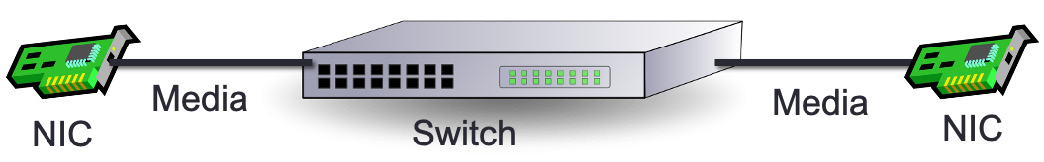
Figure 5.3 – Abstract model of a network

Every network component is essential for network latency. These are all sources of latency:

• The NIC converts the signal from a computer to a network and vice versa. The time for the NIC to process data is negligible but is not zero. The NIC is chosen for low-latency data paths and other capabilities, such as the following:
  • Bus: A bus transfers data from one component of a computer to another one. We can find three main types of buses: Peripheral Component Interconnect (PCI), PCI eXtended (PCI-X), and PCI Express (PCIe). They all have different speeds. In 2017-2018, the industry started using PCIe 5.0, working with a rate of 63 gigabytes per second (GB/s). Even though PCIe 6 was announced in 2019, PCIe 5.0 is the fastest bus for NIC.
  • Number of ports: A NIC card can have different numbers of ports: one, two, four, or six. It can allow a machine to access multiple networks at the same time. However, it is also possible to have multiple NICs on the same machine.
  • Port type: NICs can have different types of connections. A Registered Jack-45 (RJ-45) port is one type of port. It uses a twisted-pair cable named Category 5 (Cat5) or Category 6 (Cat6). The other common cable type we can have is the coaxial one, which connects to a Bayonet Neill-Concelman (BNC) port. The last one is an optical port that works with a fiber-optic cable.
  • Network speed: The standard supported network speed is single-lane 100 gigabits per second (Gbps), 25 Gbps, and 10 Gbps signaling. Anything else (that is, 400 Gbps, 50 Gbps, 40 Gbps, and so on) comprises multiple parallel lanes. Ethernet with 10 Gbps and 25 Gbps is used in data centers and financial applications every day.
  • Application-specific integrated circuit (ASIC): Integrates the functionality to interface with the host PC over PCIe and the network itself.
• Hub: A hub is a device with several ports connecting a local area network (LAN) network together. When a packet gets into the system by a port, it is replicated throughout the LAN, allowing all recipients to see all packets. A hub serves as a central connecting point for all devices in a network. This technology has been almost obsolete. Metamako/Exablaze revived this technology, and it is a latency-saving method for applications in HFTs.
• Switch: A switch works at the data link layer (layer 2) and sometimes the network layer (layer 3); therefore, it can support any packet protocols. Its main role is to filter and forward packets across the LAN.
• Router: A router joins—at a minimum—two networks and facilitates packet delivery from hosts on one network to those on the other. In an HFT system, the router is found at the gates (gateways in Chapter 2, The Critical Components of a Trading System) of the trading system. The router finds the best way to forward a packet from one host to another.

The primary components (such as routers, NICs, and switches) will introduce latency in the HFT system.

Comprehending how switches work

Switches are the primary support of communication within an HFT network. Observe the following diagram:

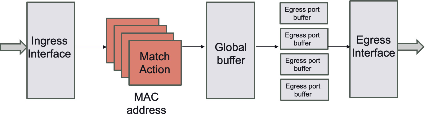
Figure 5.4 – Abstract model of a switch

Figure 5.4 represents the abstract model of a switch. Ingress and egress are words used in the industry to denote the input and output (I/O) of any network device. The switch works at the network layer 2. Its primary function is to transfer a packet from its input to its output, which you can see in the preceding diagram as Ingress Interface and Egress Interface, by applying forwarding rules. A switch handles two sorts of operations, as outlined here:

• Configuring packet forwarding: For a naive switch, the model is just to observe media access control (MAC) addresses on a port and switch traffic to that port. More sophisticated switches (that is, ones that support layer 3/4) will allow actions on other match patterns (that is, IP address or port).
• Forward/filter decisions: Switches read configuration tables to forward packets accordingly and remove packets when necessary.

The switch is set up once at startup time, and then tables are generated on the fly as new forwarding entries are required, such as when routing tables are updated.

The parser is the first to deal with new packets (the packet body is buffered independently and is unavailable for matching). The parser defines the switch's protocols, identifying and extracting information from the header.

Following that, the extracted header fields are sent to the match-action tables (component matching header fields to perform an action). Ingress and egress are separated in the match-action tables. Ingress match-action decides the egress port(s) and the queue into which the packet is routed, while both may alter the packet header. The packet may be forwarded, duplicated, discarded, or triggered by a control flow based on ingress processing. The egress match-action modifies the packet header on a per-instance basis (for example, for multicast copies). To track frame-to-frame state, action tables (counters, policers, and so on) can be linked to a flow.

Metadata, regarded similarly to packet header fields, can be carried by packets between stages. All metadata instances are the ingress port, the transmit destination and queue, and data moved from table to table without modifying the packet's parsed representation.

Beyond the network structure, the key part of the networking metrics is speed. We will define some metrics for speed in the following section.

Bandwidth, throughput, and packet rate/size

The bandwidth is the theoretical number of packets exchanged between two hosts. The pace at which communications reach their intended destination is referred to as throughput. The key distinction between the two is that the throughput measures real packet delivery rather than theoretical packet delivery. You can see how many packets arrive at their destination by looking at the average data throughput. Packets must effectively reach their destination to provide a high-performance service. It is very important to not lose any packets. If, for instance, we want to build an order book by incremental update, losing a packet means having an incoherent book.

When assessing and measuring the performance of networks, packet size and packet rate are two crucial criteria to take into account. The network performance varies depending on the settings of these parameters. The throughput value rises in proportion to packet size, then falls until it reaches the saturated value. Increasing the packet size increases the quantity of data sent, thus boosting throughput.

The following screenshot illustrates the network throughput (in kilobits per second, or Kbps) versus the packet rate (number of packets per second in bytes):

Figure 5.5 – Throughputs versus packet rate for different packet sizes

Each of the two lines shown in Figure 5.5 corresponds to a different packet size (512 bytes and 1,024 bytes). The network throughput improves when the packet rate increases because raising the packet rate means increasing the amount of data, which raises the throughput. In addition, the chart shows that as the number of packets increases, the throughput declines until it approaches the saturation point. The increase in throughput for bigger packets is faster than for smaller ones, and the peak value of throughput for 1,024-byte packets is reached at 50 packets.

When the maximum throughput of an interface is reached, multiple ingress interfaces trying to submit outbound packets to the same egress interface can lead to buffering.

Switch queuing

A switch's main function is to route packets to the proper recipients. When there is too much incoming data, the time to process data can take longer than the arrival time of this data into the switch. To not lose any data, it is essential to have a buffer. This buffer will store data waiting to be processed. The primary role of a switch is to receive a packet on the input port. It looks up the destination to get an output port and then puts the packet in the output port queue. A large data stream going toward an output port can saturate the output port queue. If too much data sits in the queue, this will result in significant latency. Data can be lost if the buffer is full (packet drops). If market data packets drop, it becomes impossible to build the order book, which interrupts trading. The following diagram depicts the queue for a switch:

Figure 5.6 – Switch queuing

One of the significant problems is head-of-line (HOL) blocking. This problem occurs when many packets are held up in a queue by a packet about to leave the queue, which can increase latency or reordering of the packets. Indeed, if many packets are blocked in one queue, the switch will keep processing other packets going toward another output; this will result in packets being received not in order.

We saw how queuing can impact packet delivery; now, we will talk about the two main switching modes.

Switching modes – Store-and-forward versus cut-through

The switch must receive and review various bytes depending on the switching mechanism before processing the packet and forwarding the packet to the correct egress port. There are two switching modes, as detailed here:

• Cut-through switching mode has two forms, as follows:
  • Fragment-free switching
  • Fast-forward switching
• Store-and-forward switching mode

Both switching types make forwarding decisions based on the destination MAC address of the Ethernet frames. They parse the bits of the source MAC address in the Ethernet header; they record MAC addresses and create MAC tables. The amount of frame data that the switch must receive and review before the frame may be transmitted out the egress port varies between switching types, as illustrated in the following screenshot:

Figure 5.7 – Switching modes based on frame bytes received

Figure 5.7 shows the three modes and represents how much information should be received. Here, we will learn about them in detail, as follows:

• Store-and-forward mode: Before forwarding the frame, the switch must receive the frame entirely. The decision to forward this frame is based on a destination MAC address lookup. To confirm the integrity and accuracy of the data, the switch uses the frame-check-sequence (FCS) field of the frame. The frame is invalid and discarded if the CRC values do not match. Before the frame is transmitted, the destination and source MAC addresses are checked to see if they match.

By default, any frame size between 64 bytes and 1,518 bytes is accepted and the other size will be discarded, resulting in a higher delay than the other three methods.

• Cut-through switching mode: This mode allows an Ethernet switch to make a forwarding choice when it receives the first few bytes of a frame. This mode has two types, as outlined here:
  • Fragment-free switching: This mode requires switches to parse the first 64 bytes of a frame before forwarding it.
  • Fast-forward switching: A cut-through switch forwards the frame when it receives the frame's destination MAC address, which implies just the first 6 bytes are required.

We saw the two main switching modes; we will now describe the different layers where switches can perform packet forwarding.

Layer 1 switching

A physical layer switch, also known as a layer 1 switch, is part of the OSI model's physical layer. A layer 1 switch may be an electronic and programmable patch panel. It does nothing more than establishing a physical connection between ports. The link is made by software instructions, allowing test topologies to be configured automatically or remotely. A layer 1 switch does not read, alter, or use packet/frame headers to route data. These switches are entirely invisible to data and have very low latency. In testing settings, transparent connections between ports are critical because they allow the tests to be as accurate as though a patch cable connected the devices. Arista/Cisco is an example of a layer 1 switch.

Layer 2 switching (or multiport bridge)

A layer 2 switch has two functionalities, as outlined here:

• Transferring data on layer 1 (physical layer)
• Checking errors for any frames that are received and sent

This type of switch needs the MAC address to forward frames to the correct recipients. All the MAC addresses received will be kept in a forwarding table. This table allows the switch to forward data in a very efficient way. Unlike higher-level switches (higher than 3) that can transfer packets based on IP addresses, a layer 2 switch cannot use IP addresses and has no prioritization mechanism.

Layer 3 switching

A layer 3 switch is a device that acts as the following:

• A router with smart IP routing by analyzing and routing packets based on the source and destination addresses
• A switch linking devices on the same subnet

We will now talk about the system that is capable of routing data from many private IP addresses using a public address.

Network address translation

The process of converting private IP addresses into public addresses is known as network address translation (NAT). Most routers employ NAT to allow many devices to share a single IP address. When a machine communicates with the exchange, it looks for directions to the exchange. This request is sent as a packet from a machine to the router, forwarding it to the business. The router must first transform the source IP address from a private local address to a public one. The receiving server will not know where to send the information back if the packet contains a private address. The information will be returned to the laptop using the router's public address rather than the laptop's private address, thanks to NAT.

NAT is a resource-intensive operation for any device that uses it. This is because NAT requires reading and writing to the header and payload information of every IP packet to accomplish address translation, which is a time-consuming process. It increases the consumption of the central processing unit (CPU) and memory, which might reduce throughput and increase packet delay. As a result, while installing NAT in a live network, knowing the performance impact of NAT on a network device (specifically, a router) becomes critical, especially for HFT. Most modern switches can perform at least static NAT in an ASIC, but an increasing number can also do dynamic NAT with a little performance penalty.

We studied in detail how to transmit packets. We will now describe the protocols setting the rules for packet forwarding.

Important protocol concepts

When two devices need to communicate, once they have a way to transfer a signal from the sender to the recipient, we need to have protocols setting the communications rules. A protocol is like a language that two components agree to use in the system to communicate; it sets the rule of communication. The following diagram represents a network infrastructure of exchanges and trading systems:

Figure 5.8 – Trading network infrastructure of trading exchange and trading servers

In Chapter 2, The Critical Components of a Trading System, and Chapter 3, Understanding the Trading Exchange Dynamics, we saw that the trading exchange, market data-feed handlers, and market participants are the three main components of a conventional trading system.

Through gateway servers, the matching receives orders from market participants. The feed handlers get their data from the stock exchange and deliver it to interested market players with minimal delay. To transport market data, we use the FIX Adapted for STreaming (FAST) protocol (described later in the FAST protocol section).

We will now talk about the Ethernet protocol for HFTs.

Using Ethernet for HFT communication

Ethernet is the most used protocol to link devices in a wired LAN or wide area network (WAN). This protocol sets the communication rules between devices.

Ethernet specifies how network devices structure and send data so that it may be recognized, received, and processed by other devices on the same LAN or company network. This protocol is highly reliable (resistant to noise), fast and secure, and was designed by the Institute of Electrical and Electronics Engineers (IEEE) 802.3 working group in 1983. The technology kept improving to get a better speed.

The different norms—802.3X and 802.11X—defined another type of support, such as 100BASE-T, which has been named Fast Ethernet that we are still using today.

Using IPv4 as a network layer

The IP protocol operates at the OSI model's network layer while TCP and UDP models operate at the internet layer. As a result, this protocol is in charge of recognizing hosts based on their logical addresses and routing data between them through the underlying network.

An IP addressing system offers a technique for uniquely identifying hosts. IP utilizes best-effort delivery, which means that it cannot promise that packets will be sent to the intended host, but it will try its hardest to do so. The logical address in IPv4 is 32 bits.

We can use three different addressing modes when using the IPv4 protocol, as detailed next.

Unicast mode

Only one designated host receives data in this manner. The 32-bit IP address of the target host is stored in the Destination Address field. In this case, the client transmits data to the desired server, as illustrated in the following diagram:

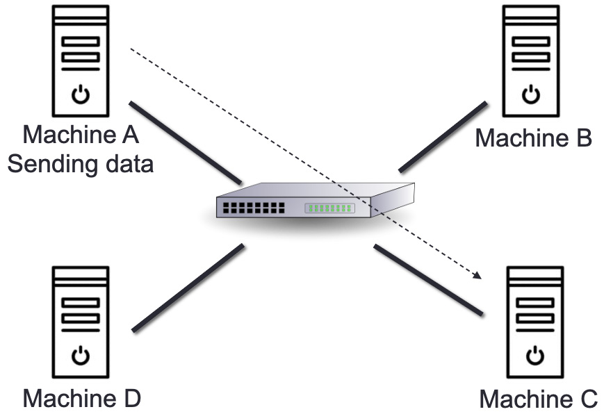
Figure 5.9 – Unicast mode

As seen in the preceding diagram, Machine A sends information to Machine C.

Broadcast mode

The packet is addressed to all hosts in a network segment in this mode. A specific broadcast address, 255.255.255.255, is included in the Destination Address field. When this packet is seen on the network, a host is obligated to process it. In this case, the client transmits a packet received by all of the servers. Broadcast is rarely used in HFT systems because it gives you almost no control over which machines will receive traffic and could create unnecessary overhead. You can see an illustration of broadcast mode in the following diagram:

Figure 5.10 – Broadcast mode

As seen in the preceding diagram, Machine A sends information to all the machines.

Multicast mode

This mode is a hybrid of the previous two in that the packet is transmitted to neither a single host nor all of the hosts on the segment. The Destination Address field in this packet has a unique address that starts with 224. x.x.x and can be served by several hosts. Hosts will subscribe to particular multicast feeds. A machine communicates to the upstream service using the Internet Group Management Protocol (IGMP) that it wishes to subscribe to a specific feed. Many switches have the logic that monitors IGMP traffic from hosts and snoops on subscriptions for feeds. This enables the switch to determine which hosts it should replicate multicast traffic to. Switches that don't implement IGMP snooping treat multicast traffic like broadcast traffic. You can see an illustration of multicast mode in the following diagram:

Figure 5.11 – Multicast mode: Machine A sending information to Machine B and C

In this section, we reviewed the network layer and its components. We will now talk about the transport layer and the UDP and TCP protocols.

UDP and TCP for the transport layer

TCP/IP or UDP over Ethernet is the most common communication protocol used by stock exchanges and other market players. Non-essential data, such as market data feeds, is often transmitted using UDP to reduce latency and overhead. One of the most important protocols in the TCP and UDP protocol family is IP. Critical data such as orders is carried out using the TCP/IP protocol.

TCP specifies how a computer is connected to another machine and how we can transmit data between them. This protocol is reliable and provides an end-to-end (E2E) byte stream over the network.

A datagram-oriented protocol (UDP) is used for broadcast and multicast types of network transmission. UDP is different from TCP as it does not ensure packet delivery.

The main differences are outlined here:

• TCP is a connection-oriented protocol, and UDP is a connectionless protocol.
• Because UDP doesn't have any mechanism to check errors, UDP is faster than TCP.
• TCP needs a handshake to start communicating while UDP does not.
• TCP checks errors and has error recovery, while UDP checks for errors and discards packets when there is a problem.

UDP doesn't have TCP's session, ordering, and delivery guarantee features. UDP is used where latency matters because data is delivered on a datagram basis. Market data often uses it for one of two reasons, as outlined here:

• Datagram-oriented delivery can be lower-latency (but recovery is more complicated if something gets lost).
• Multicast inherently does not support connection-oriented protocols (since the traffic is a many-to-many communication type).

This is often addressed through sequence numbers in the application-layer protocol and providing an out-of-band mechanism to request retransmission of missing sequence numbers. Today, there is a trend to use UDP for Orders (UFO), which allows us to send orders faster.

Designing financial protocols for HFT exchanges

Let's come back to the following diagram, introduced in Chapter 2, The Critical Components of a Trading System. It is important to understand how communication works between a trading system and an exchange:

Figure 5.12 – Communication between exchange and trading system

Two entities must speak the same language to communicate with one another. To accomplish that, they use a protocol used in networking. This protocol is utilized in trading for any exchanges (sometimes called venues). Depending on the venue, there may be a variety of protocols. The connection is possible if the protocol between a given venue and your trading system is the same. Depending on the number of venues, one venue will frequently use a given protocol, and another venue will use a different one. The trading system will need to be built on understanding the other protocols. Even though their protocols differ among venues, the processes they take to create a connection and begin trading are similar, as outlined here:

1. They establish a logon that specifies who the trade initiator is, who the recipient is, and how the connection will continue to exist.
2. They next enquire about what they expect from the various companies, such as trading or receiving price updates by subscription.
3. They then get orders as well as pricing changes.
4. They then send heartbeats to sustain a connection.
5. Finally, they say their goodbyes.

We will now introduce the Financial Information eXchange (FIX) protocol in the following section.

FIX protocol

Because it is the most used protocol in trading, the Financial Information eXchange (FIX) protocol is the one we'll be discussing in this chapter. It was founded in 1992 to handle securities between Fidelity Investments and Salomon Brothers on an international real-time exchange. Foreign exchange (FX), fixed income (FI), derivatives, and clearing were included. This is a string-based protocol, which implies that people can read it. It's platform-agnostic, open, and comes in a variety of flavors.

There are two different kinds of messages, as outlined here:

• Administrative notifications that do not include any financial information
• Messages sent by the program to get pricing changes and orders

The content of these messages is a list of key-value pairs, similar to a dictionary or a map. Predefined tags serve as the keys; each tag is a number that corresponds to a particular characteristic. Values, which might be numerical or textual values, are associated with these tags. Consider the following scenario:

• If we wish to send an order for $1.23, let's imagine the price tag has the number 44. As a result, 44=1.23 will be in the order message.
• Character 1 separates all of the pairs. This indicates that if we add the quantity 100,000 using tag 38 corresponding to the quantity in the FIX message definition in our previous example, we'll get 44=1.23|38=100000. The | symbol symbolizes character 1.
• 8=FIX.X.Y is the prefix used in all messages. This prefix denotes the FIX version numbers. Version numbers are represented by X and Y.

10=nn is equal to the checksum. The checksum is the total of the message's binary values. This aids in the detection of infection.

Here is a FIX message example:

8=FIX.4.42|9=76|35=A|34=1|49=TRADER1|52=20220117-12:11:44.224|56=VENUE1|98=0|108=30|141=Y|10=134

The necessary fields in the preceding FIX message are listed here:

• A tag containing the number 8 and the value FIX.4.42. This is the same as the FIX version number.
• 8 (BeginString), 9 (BodyLength).
• 35 (MsgType), 49 (SnderCompID), and 56 (SnderCompID) are version numbers greater than FIX4.42.
• The tag 35 specifies the message type.
• The character count from tag 35 to tag 10 is represented by the body-length tag, which is 9.
• The checksum is stored in field 10. The value is derived by multiplying the decimal value of the American Standard Code for Information Interchange (ASCII) representation of all bytes up to the checksum field (which is the final field) by 256.

Now that we know what the FIX protocol is, we will see in detail how this protocol is used in trading.

Protocols for FIX communication

To be able to trade, a trading system requires two connections: one to receive price updates and another to place orders. The FIX protocol complies with this criterion by utilizing different messages for each of the following connections.

We will discuss the price changes connection first and then describe the order connection.

Price changes

When building a trading system, the first feed to get is price updates. Price updates are the orders from the other market participants. The trading system will initiate a connection with the exchange to get a connection established and subscribe to the price updates. We will define the trading system as the initiator and the exchange as the receiver or acceptor, as depicted in Figure 5.13.

Trading systems require prices for the instruments that traders choose to trade. To do so, the trading system establishes a connection with the exchange to subscribe to liquidity updates. The connection between the initiator, which is the trading system, and the acceptor, which is the exchange, is depicted here:

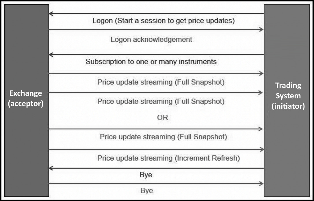
Figure 5.13 – Trading system asking for price updates

The FIX messages that are sent between the acceptor and the initiator are depicted in the following screenshot:

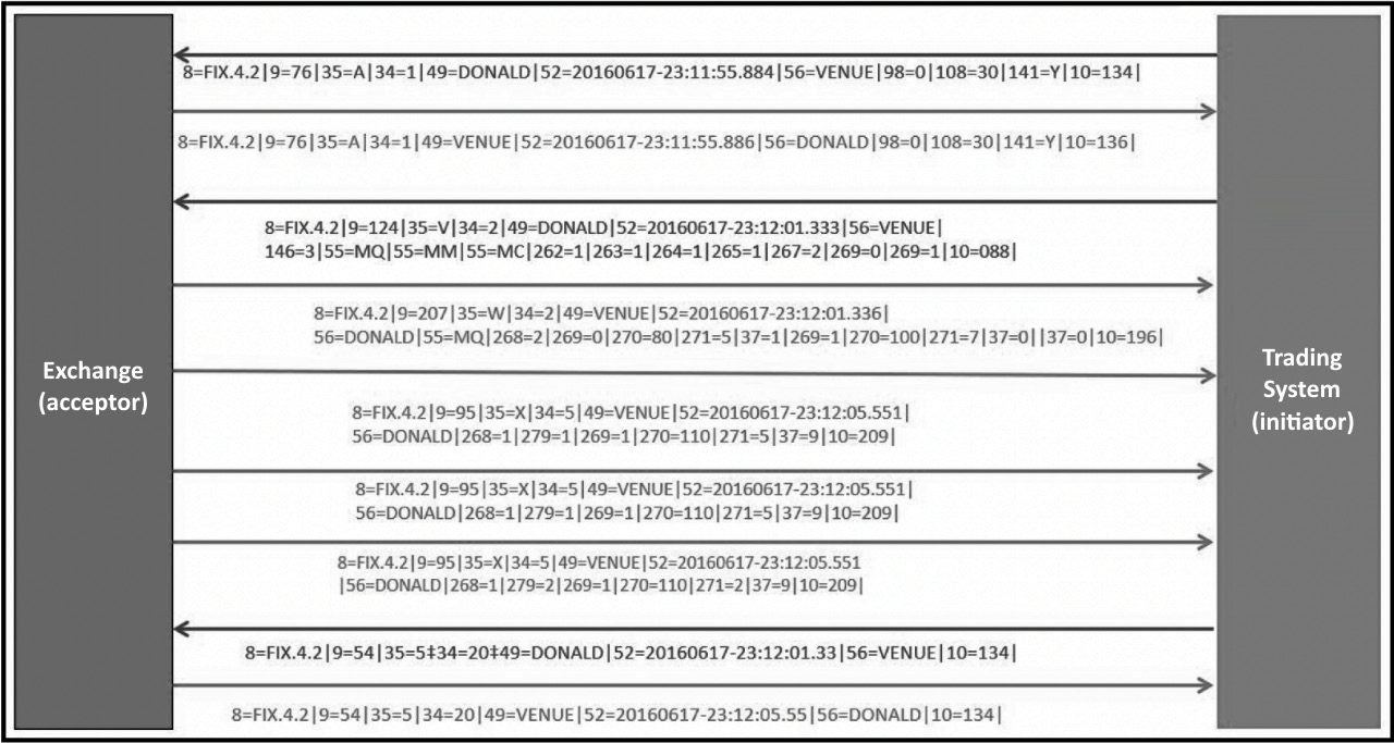
Figure 5.14 – Trading system using FIX protocol to get price updates

When the trading system receives these price updates, it updates the books and places orders depending on the signal.

Orders

The second feed that a trading system needs is communication with the exchange for the order side. The trading system (initiator) will establish communication with the exchange (receiver). Once the communication is established, the initiator will send orders to the exchange. When the exchange needs to send updates about an order, it will use this channel to communicate.

By initiating a trading session with the exchange, the trading system will send orders to the exchange. Order communications will be delivered to the exchange while this active trading session is open. The exchange will use FIX messages to transmit the status of these orders. This is depicted in the following diagram:

Figure 5.15 – Trading system sending an order to the exchange

The FIX messages that are sent between the initiator and the acceptor are depicted in the following screenshot:

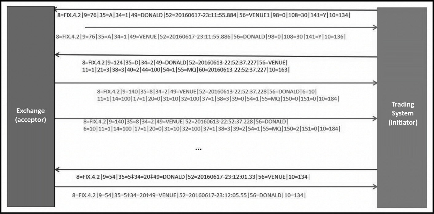
Figure 5.16 – A trading system using the FIX protocol to send an order to the exchange

Because the FIX protocol is string-based, parsers can take some time to process the stream. The FAST protocol has been developed to be faster than the FIX protocol.

FAST protocol

The FAST protocol is the high-speed version of the FIX protocol. Market data is transmitted from exchanges or feed handlers to market participants via the FAST protocol, which operates on top of UDP. FAST messages feature a variety of fields and operators for transporting meta- and payload data. FAST has been designed to use as little bandwidth as possible. Hence, it makes use of a variety of compression techniques, as outlined here:

• The first essential approach is delta updates, which offer just changes—such as the current stock price and the previous one—rather than continually transferring all stocks and their accompanying data.
• The second approach uses variable-length encoding for each data word to compress the raw data. While these strategies allow for keeping up with the increased data speeds given by feed handlers, they significantly increase processing complexity.

The compressed FAST data stream must be decoded and analyzed in real time to convert it into processable data. If the processing system cannot keep up with the data flow, critical information is lost.

Furthermore, decompressing the data stream increases the amount of bandwidth that must be handled successfully. As a result, two distinct criteria must be met to design a high-performance trading accelerator, as follows:

• First, the various protocols' decoding must be done with the shortest possible delay.
• Second, it must sustain data processing at a given data rate. A deeper look at the FAST protocol is necessary to examine the data rates of modern trading systems.

The UDP protocol is used to send FAST messages. Multiple FAST messages are packed in a single UDP frame to decrease UDP overhead. FAST communications do not provide any size information or a framing definition. Instead, each letter is specified by a template that must be understood before decoding the stream. Most feed handlers design their FAST protocol by offering distinct template requirements. Care must be taken because a single decoding error will drop the entire UDP frame. Templates define a set of fields, sequences, and groups. These groups specify a set of fields.

FAST belongs to a family of protocols developed to improve the bandwidth and the speed of communication named Simple Binary Encoding (SBE). We will now talk about protocols that are way more efficient than string-based protocols for communication.

ITCH/OUCH protocol

ITCH and OUCH are considered binary protocols. OUCH is usually over TCP, and ITCH is multicast or TCP. ITCH is mainly for market data, while OUCH is made for the orders. Nasdaq created these protocols in 2000 after a patent infringement lawsuit impacted FAST. ITCH-based exchange feeds are widely used in the industry. Because many different exchanges than Nasdaq use it, it has different versions. The Chicago Board Options Exchange (CBOE) is also another major exchange that heavily uses a variant of ITCH (such as the CBOE protocol).

Let's study another one—the Chicago Mercantile Exchange (CME) market data protocol.

CME market data protocol

CME also created its SBE protocol optimized for HFT.

Additionally to the prior protocols, many other proprietary binary protocols are famous for low-latency venues. All these protocols are considered exterior protocols that are responsible for connecting/interacting with exchanges. We will now talk about the difference between exchange protocols made for exterior networks and protocols made for internal networks.

Interior networks versus exterior networks

When looking at Figure 5.8, we can observe two different levels of the network. There is the level of network talking to the outside world using the prior protocols, and there is the networking within the company network (interior network). The following diagram illustrates the main difference between the exterior and internal networks in trading and exchange networks:

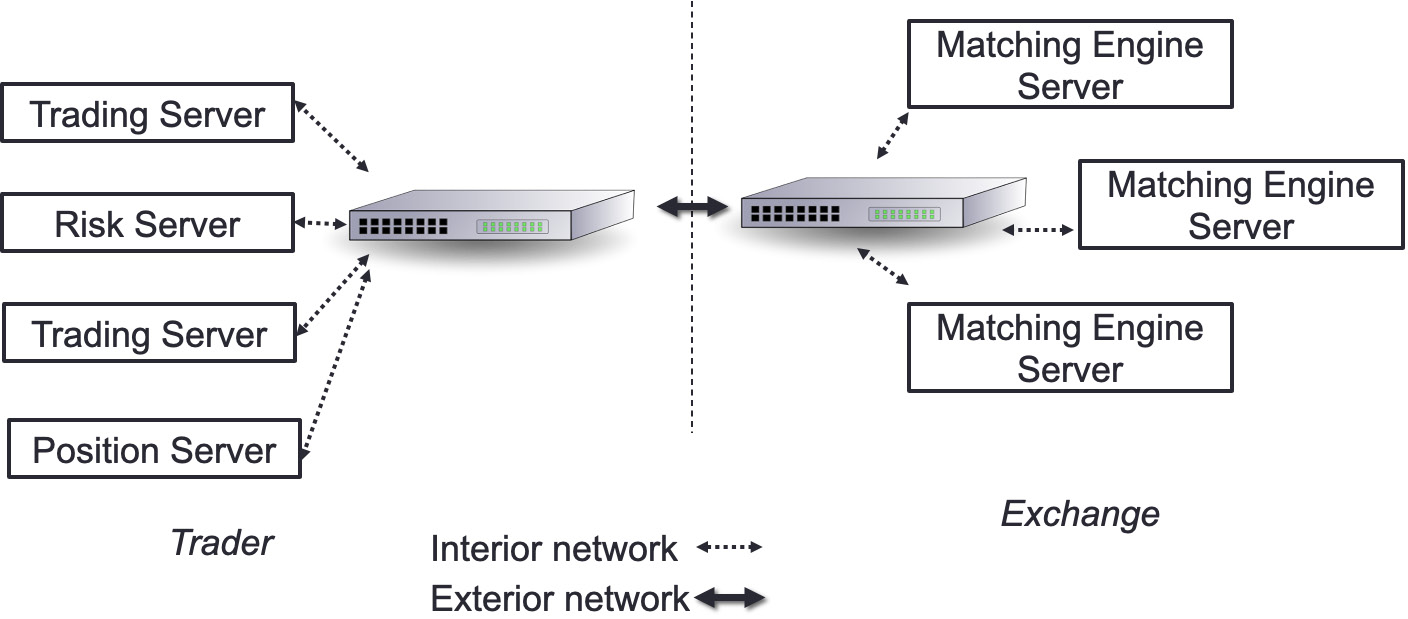
Figure 5.17 – Interior network and exterior network

A trading server communicating with the risk server uses the interior network, while the trading system on the left side of the preceding diagram will be connected with the exchange through the external network.

The internal network will be for the following activities:

• Internal market data distribution
• Signal sharing
• Order entry

It is essential in this network to minimize hops between hosts (servers). The best system will be a system where there is a segue into systems that exist purely on the NIC (in other words, a field-programmable gate array (FPGA), which we will discuss in Chapter 11, High-Frequency FPGA and Crypto. The choice of switches and routers is decisive for the network latency.

The external network will be for the exchange native protocol for order entry and market updates.

We are now aware of which network can be considered interior and exterior. We also know which hardware a packet will use to go from one place to another. In the next section, we will describe the structure of a packet and dig further into the life cycle of a packet and what happens as a packet moves from one point to the other.

Understanding the packet life cycle

In the Learning about network conceptual models section, we explained that to optimize the communication between the exchange and trading systems, we will use copper or optical wire. This wire is connected to the NIC. This wire will transport the packets containing market data from the exchange and orders going to the exchange.

We first need to discuss which message we are passing on this wire. This section will use the FIX protocol we defined in this chapter. Let's consider the following example of a FIX message:

8=FIX.4.2|9=95|35=X|34=5|49=NYSE|52=20160617-23:12:05.551|56=TRADSYS|268=1|279=1|269=1|270=110|271=5|37=9|10=209|.

This FIX message will be the payload of the packet shown in Figure 5.18.

The packet has two main parts. The headers contain information for each layer of the OSI model and a payload containing the FIX message, as shown here:

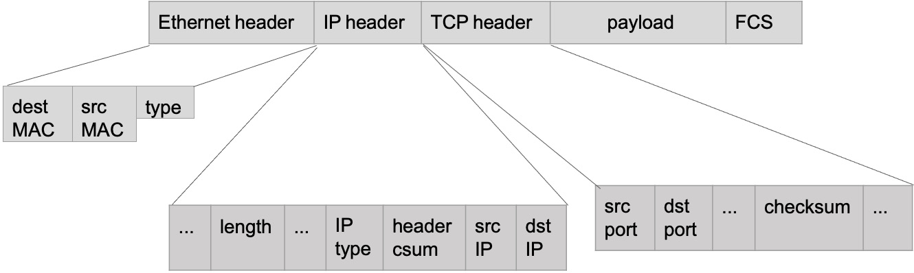
Figure 5.18 – Packet headers

The Ethernet layer will represent the data link layer (as shown in Figure 5.19), the IP header for the network layer, and the TCP header for the transport layer. The FCS is an error-detecting code added to this packet. As we described earlier, each layer of a packet (or a frame) contains information for each layer. We will specify in Figure 5.20 how this packet is processed in the machine, but first, observe the following diagram:

Figure 5.19 – Headers and OSI layers

In the following diagram, you can follow the life of a packet carrying a market data update getting through the system to reach the trading system (one of the applications running on this architecture):

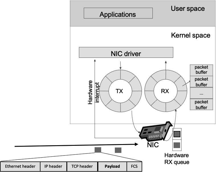
Figure 5.20 – Market data moving through the operating system

We will talk in detail about all the necessary steps to get the packet from the wire to the application—our trading system. We will first talk about the send/receive path.

Comprehending the packet life in the send/receive (TX/RX) path

The exchange connected to the trading system sends a packet to the trading system. The copper wire will transfer this packet to the machine. Here are the steps that the packet will follow:

1. The NIC receives the packet and verifies if the MAC address (unique identifier (UID) assigned to a NIC) address corresponds to its MAC address. If that is the case, this NIC will process this packet.
2. Then the NIC validates that the FCS is correct (checksum operation).
3. When these two verifications are completed, the NIC will use a direct memory access (DMA) operation to copy the packet to the buffer in charge of receiving data (receive (RX) buffer).
4. In Figure 5.20, the RX buffer is a circular buffer (or ring buffer), which is a data structure using a fixed-size buffer, connected E2E (mainly used to avoid using locks). DMU speeds up memory operations by allowing an I/O device to transmit or receive data directly to or from the main memory, bypassing the CPU.
5. The NIC then triggers an interrupt for the CPU to take care of this packet. Interrupt handlers are typically broken up into two halves—a top half and a bottom half. The top half handles any work that needs to be done urgently, and the bottom half deals with all other processing. The top half will manage activities such as acknowledging the interrupt and moving data from the network to a buffer for subsequent processing by the bottom half. The processor will switch from the user space to the kernel space, look up the interrupt descriptor table (IDT), and calls the corresponding interrupt service routine (ISR). Then, it will switch back to the user space. These operations are done at the NIC driver level.
6. The CPU will then initiate the bottom half when free (the soft interrupt request (soft-IRQ)). We will switch from the user space to the kernel space. The driver allocates a socket buffer or SK-buff (also called SKB). The SKB is an in-memory data structure containing the packet headers (metadata). It includes pointers to the packet headers and, obviously, the payload. For all packets in the buffer (RX buffer), the NIC driver dynamically allocates an SKB, updates the SKB with the packet headers, removes the Ethernet header, and then passes the SKB to the network stack. The socket is the endpoint to send and receive data on the software level.
7. We will now address the network layer. We know that the network layer contains the IP address. This layer will verify the IP address and the checksum and remove the network header. When verifying the IP address, the address will be compared against the route lookup. If some packets are fragmented, this layer would be in charge of recombining all the fragmented packets. Once this is done, we are taking care of the next layer.
8. The transport layer is specific to the TCP (or UDP) protocol. This layer handles the TCP state machine. It will enqueue the packet data to the socket read queue. Then, at the end, it will signal that a message can be read in the reading socket.

We will conclude this section by talking about the software layer in charge of writing and reading network data.

Software layer receiving the packet

Once the payload is written in the reading socket named read queue, the only missing step is to have the application (trading system) read the payload. We know that the operating system schedules the application to read data from the socket when possible (fairness rules). Once the trading system (the application) reads the payload (which is in this example the FIX message in the Understanding the packet life cycle section), it will start parsing the different tags and values of the message.

When we review all the steps that a trading system must do just to read market data, HFT is predominantly concerned with the amount of time required for an operation to complete in microseconds or nanoseconds. Therefore, we will see how to improve this path.

Since the network is critical in terms of speed, we need to be able to monitor it. In the next section, we will talk about monitoring techniques.

Monitoring the network

The network is critical for HFTs. Saving microseconds from the critical path to send orders in the network is key. When the network is built and the system is running, it is essential to analyze network traffic. In HFT, security is not a real issue since the network is located in a co-location most of the time. The part of the monitoring that we will give more weightage to is analyzing the amount of data loss, latency, and interruption. We need to ensure that the network is up and running and delivers the best possible performance.

Packet capture and analysis

Capturing Ethernet frames for examination or analysis is referred to as packet capture. The word can also refer to the files produced by packet-capture programs, commonly saved in the .pcap format. Capturing packets is a typical network troubleshooting tool, and it's also used to look for security vulnerabilities in network traffic. Packet captures give crucial forensic information that enhances investigations following a problem with the number of orders rejected, which could seem like a network latency problem.

What is packet capture and how does it work?

A packet can be caught in a variety of ways. Packet captures can be performed via networking equipment such as a router or switch with specific hardware known as a test access point (TAP) (which we will describe in the following section). The final aim determines the method utilized. Regardless of the mechanism used, packet capture works by creating copies of some or all packets traveling through a given place in the network.

The simplest method to get started is to capture packets from your system, but there are a few limitations. Network interfaces handle only traffic destined for them by default. You can put the interface in promiscuous mode or monitor mode for a more comprehensive view of network activity. Remember that this method only captures a portion of the network. For example, on a wired network, you'll only observe activity on the local switch port to which your computer is attached.

Port mirroring, port monitoring, and switched port analyzer (SPAN) are capabilities on routers and switches that allow us to duplicate network traffic and transmit it to a specific port. Much network equipment has a packet-capture feature that may be used to diagnose problems directly from the hardware's command-line interface (CLI) or the user interface (UI).

A dedicated network TAP can be ideal for doing a packet capture on a particularly big or busy network. TAPs are an expensive way to collect packets, but there is no performance impact because they are dedicated hardware. To make the TAP effective, it is necessary to capture both directions (transmit (TX) and RX). We need to tap both the RX and TX side to build a complete picture.

Ethernet TAPs – passive versus active TAP trade-offs

A network TAP is the most precise technique to reproduce traffic for monitoring and analysis. There are a variety of network TAPs, each with its own set of advantages for network uptime and analytical dependability. This method can be passive and active network TAPs. The distinctions between passive and active TAPs might be perplexing.

Passive network TAP

A device with no physical separation between its network ports is referred to as a passive network TAP, as shown in the following diagram. This implies that traffic can continue to flow across network ports, maintaining the connection even if the device loses power:

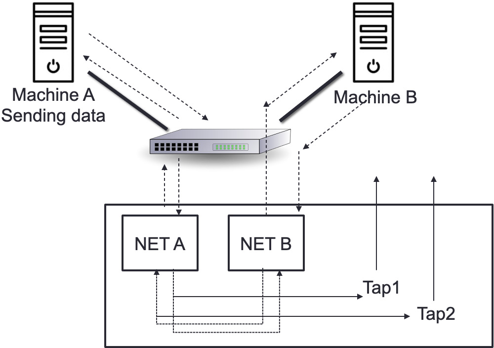
Figure 5.21 – Passive network TAP

This is true for network TAPs with 10/100-meter (10/100M) copper interfaces and fiber TAPs. Fiber TAPs work by dividing the incoming light into two or more pathways and do not require electricity. When utilized, 10M or 100M copper TAPs require electricity, although they are entirely passive due to a lack of physical separation between network ports. In their situation, the link remains operational during a power loss with no failover time or link restoration delay.

Active network TAP

Because of the electrical components utilized inside the TAP, active TAPs have a physical separation between network ports, unlike passive TAPs. As a result, they require a fail-safe mechanism to ensure that the network remains operational even if the TAP loses power. The system works by keeping a set of relays open when the gadget is turned on. These relays switch to a direct traffic flow through the TAP when the power goes out, ensuring that the network operates. You can see an illustration of this in the following diagram:

Figure 5.22 – Passive network TAP

These two TAPs will help capture market data to analyze latency and troubleshoot issues in the network. Getting this data will not be sufficient if the time of this data is not accurate. It is essential in HFT to measure time accurately. In the next section, we will explain how to do so.

Valuing time distribution

As you certainly understood with this book, HFT fights with time. This is the most critical resource we have to be sure to get our trading models right. Because we send orders that can be executed or not depending on the arrival time, we need to be confident when we build trading strategies that the time we will use to make them fits the time that the exchange is using. We will need to use time-synchronization services to accomplish this measurement accuracy.

Time-synchronization services

Before starting this section, we need to talk about getting precision time. Anywhere in the world, we can have precise time without engineering timing distribution. We use the Global Positioning System (GPS) or the Global Navigation Satellite System (GNSS), as they use atomic clocks.

The Network Time Protocol (NTP) service is one of the most widely used to synchronize the uptime of our computers with a time server. This service has a few layers called strata, as described in more detail here:

• Stratum 0: The highest layer, this uses GNSS satellites
• Stratum 1: The layer that gets the time servers, having a one-on-one direct connection with the stratum 0 clock. You can accomplish a microsecond-level synchronization with this layer.
• Stratum 2: The layer that connects to multiple servers of stratum 1.

There are up to 15 layers that help get different types of accuracy. The returned timestamp is as large as a 64-bit timestamp and can accurately be in the order of picoseconds. There will be a day in the near future when a 128-bit timestamp will be in place, and we might even get an accuracy of femtoseconds.

The Precision Time Protocol (PTP) is a network-based time synchronization standard that strives for nanosecond—or, perhaps, picosecond—precision. PTP equipment employs hardware timestamping rather than software, and it is designed for one unique purpose: keeping devices synchronized. PTP networks provide far higher time resolutions than NTP networks. PTP devices, unlike NTP devices, will timestamp the amount of time synchronization messages spend in each device, allowing for device latency.

These two synchronization mechanisms use pulse-per-second (PPS) signals from satellites, giving high accuracy. These signals have an accuracy going from 12 picoseconds to a few microseconds per second.

Why does timing matter so much in HFT?

When inserting timestamps in orders, HFTs require accurate Coordinated Universal Time (UTC) to follow orders in the market. Most HFTs run many computer systems on dedicated LANs, with each LAN utilizing a single PTP grandmaster clock and each computer on the LAN synced to that grandmaster. A grandmaster takes its time from an external source, and it is necessary to have a grandmaster per physical location. These parallel, high-speed computer systems must be coordinated for the algorithms to handle market buy-side and sell-side data. In network analysis of log files and all trading activity, timestamps and computer synchronization are also utilized.

Understanding and analyzing LAN latency is critical to HFT performance. HFTs would struggle to optimize both hardware and software if time synchronization were not exact to the microseconds. For non-co-located traders, real-time market data travels via cables, switches, and routers, with a delay ranging from 1 millisecond to 5 milliseconds. When compared to traders who are not co-located, co-located HFTs cut latency to below 5 microseconds, allowing them a substantial amount of time to process market data.

It is critical to measure market behavior and algorithm signals accurately, therefore the accuracy of measurement must be very high.

Summary

During this chapter, we talked about the importance of communication and networking. We learned about the network components of HFTs. We talked in depth about the Ethernet protocols adapted to fast communication. We described the design of financial protocols, and we finished by talking about the value of time distribution. You are now equipped with the knowledge to understand networking in HFT.

In the next chapter, we will finally start talking about how to optimize all the pieces of the puzzle we talked about during this chapter and the previous chapters.