Chapter 7: HFT Optimization – Logging, Performance, and Networking

In the previous chapter, we investigated a lot of lower-level HFT optimization tasks and optimization tips and techniques. In this chapter, we will continue the discussion and look at more topics in HFT optimization. The focus here will be on kernel and user space operations and optimizations related to them. We will also explore kernel bypass as well as optimization topics related to networking, logging, and measuring performance.

Some of the operations and constructs that we will discuss will be memory, disk, and network access operations at the operating system (OS) and server hardware levels and network architectures between data centers in different physical locations (microwave/fiber options). We will also discuss topics related to logging and statistical metrics around real-time performance measurement. Including the topics covered in the last chapter, by the end of this chapter, you will have a very good understanding of all the modern performance optimization tools, technologies, and techniques involved in HFT trading architectures.

In this chapter, we will cover the following topics:

• Comparing kernel space and user space
• Using kernel bypass
• Learning about memory-mapped files
• Using cable fiber, hollow fiber, and microwave technologies
• Diving into logging and statistics
• Measuring performance

  Important Note

  In order to guide you through all the optimizations, you can refer to the following list of icons that represent a group of optimizations lowering the latency by a specific number of microseconds:

  : Lower than 20 microseconds

  : Lower than 5 microseconds

  : Lower than 500 nanoseconds

  You will find these icons in the headings of this chapter.

It is important to understand these topics well since no modern HFT system is complete without incorporating these techniques to maximize performance. Understanding these topics is essential to building a competitive HFT business.

Comparing kernel space and user space

We touched upon the concepts of kernel and user space in the previous chapter. To refresh our memory, some privileged commands/system calls can only be made from kernel space, and this design is intentional so that errant user applications cannot harm the entire system by running whatever commands they want. The inefficiency from the perspective of an HFT application is that if it needs to make system calls, it requires a switch to kernel mode and possible context switches, which slows it down, especially if the system calls are made quite often on the critical code path. Let's formally wrap up the discussion in this section.

What is kernel and user space?

The kernel is the core component of all modern OSs. It has access to all the resources – memory, hardware devices, and interfaces, essentially everything on the machine. Kernel code has to be the most tested code that is allowed to run in kernel mode or kernel space to maintain machine stability and robustness. User space is where normal user processes run. The OS kernel still manages user space applications and polices the resources they are allowed to access. The virtual memory space is also divided into kernel space and user space. While the physical memory does not distinguish between the two spaces, the OS controls access. User space does not have access to kernel space, but the reverse is true, that is kernel space has access to user space. The diagram that follows will help you to understand the layout of these components:

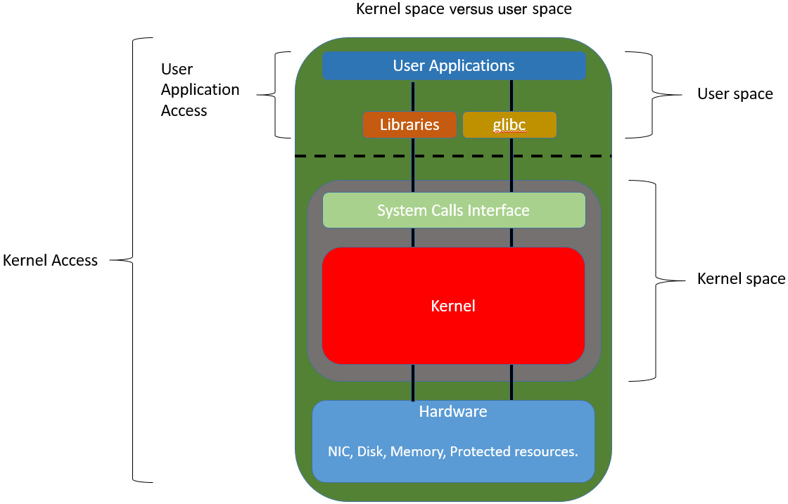
Figure 7.1 – Communication between kernel space and user space components

When processes running in user space need to execute system calls such as disk I/O, network I/O, and protected mode routine calls, they do so via system calls. In that design, system calls are the part of the kernel interface exposed by the kernel to user space processes. When a system call is invoked from a user space process, first an interrupt is sent to the kernel for the system call. The kernel finds the correct interrupt handler for the system call and launches the handler to handle the request. Once the interrupt handler is finished, processing continues onto the next set of tasks. This is not the only case where there are switches made between kernel and user space; some instructions invoked by a process running in user space also force a transition into kernel mode. For most systems, this switching does not invoke a context switch, but for some systems that might happen when switching between user and kernel mode.

Investigating performance – kernel versus user space

In general, code that runs in kernel space runs at the same speed as code in user space. The difference in performance comes into play when system calls are made – code executing in kernel space executes more quickly when system calls are involved and code executing in user space executes more slowly since when it encounters a system call, it needs to switch to kernel/supervisor mode and that switch is slow and can trigger even more expensive context switches. So, for user applications, it makes sense to minimize the use of system calls and try to eliminate them altogether if possible.

Another example is gettimeofday() and clock_gettime(), which, under the hood, invoke system calls. Since HFT applications update time very frequently, this can add up to a lot of system calls. Alternatives to that approach that would eliminate system calls are rdtsc() instructions, and on some architectures, even chrono time calls are able to avoid system calls.

Overall, there can be many opportunities during HFT application development where it is possible to eliminate or minimize (the latter being more realistic) system calls invoked from the user space application. You just need to give some thought to what methods are being called, if they invoke system calls, and if there is a better way to have the same functionality but without invoking system calls – at least as far as code in the critical hot path is concerned.

We will see an example of eliminating system calls in the section on Learning about memory-mapped files. By loading up the file into memory and allowing the processes to make changes directly to the memory and delay/throttle how often changes get committed to disk, the design minimizes system calls. Another example of eliminating systems calls altogether for network read/write operations is kernel bypass, which we will discuss shortly in the Using kernel bypass section.

We will discuss the latency improvements achieved by using that technique; however, you should know that a part of the improvement is achieved by eliminating unnecessary copies of data buffers. Before we look into the details, we will present some data here regarding the improvements. UDP read/write times without kernel bypass range between 1.5 to 10 microseconds, and with kernel bypass, range between 0.5 and 2 microseconds. TCP read/write times also have similar performance increases, except a tiny bit slower. Let's start by discussing the details of kernel bypass technology and its benefits next.

Using kernel bypass

In this section, we will discuss using the kernel bypass technique to improve the performance of User Datagram Protocol (UDP) sockets to process inbound market data updates from the exchanges and Transmission Control Protocol (TCP) sockets to send outbound order flow/requests to the exchange. Fundamentally, kernel bypass looks to eliminate the expensive context switches and mode switches between kernel mode and user mode as well as duplicate copying of data from the Network Interface Card (NIC) to user space, each of which ends up reducing the latency quite a bit.

Network processing driven by system calls/interrupts in the non-kernel bypass design, threads, or processes that want to read incoming data on UDP or TCP socket block on the read call, as described in the Understanding context switches – interrupt handling section in the previous chapter. That leads the blocked thread or process being context switched out, and then it is woken up by the interrupt handler when data is available on the socket. We discussed in the previous chapter, how the context switching of threads and switches between kernel mode to user space are inefficient since it adds latency on every single packet read.

For HFT applications that process market data and order responses, millions of such packet reads occur throughout the day and hence the delay adds up and causes significant performance degradation. Additionally, data is copied from the NIC buffers from kernel space to application buffers in user space, so the additional copy is another source of latency. A similar copy mechanism exists on outgoing UDP or TCP packets (TCP is the most common protocol for HFT applications, but outgoing UDP packets can exist depending on how the applications are designed).

Understanding why kernel bypass is the alternative

The alternative to eliminate the latencies incurred in traditional socket programming, which make it a bad fit for HFT, has two aspects: spinning on a CPU core in user space and zero copy of incoming and outgoing data. Both require special NICs and accompanying Application Programming Interfaces (APIs) that support these features – some examples are Solarflare NICs and the OpenOnload/TCPDirect/ef_vi API to support kernel bypass, Mellanox NICs and Mellanox Messaging Accelerator (VMA) APIs, and Chelsio adapters and WireDirect/TCP Offload Engine (TOE) APIs. Let's look at them in more detail in the following sections.

User space spinning

The alternative to the blocking and context switching design is for the calling thread or process to spin in user space while constantly polling the UDP and/or TCP sockets that are enabled for kernel bypass. This comes at the price of constantly polling and utilizing 100% of the CPU core. The good news is that polling is strictly in the user space, that is, no system calls or kernel time and CPU cores are plentiful in modern HFT trading servers, so this is a good trade-off. In this design, the NIC buffer mirrored into user space is polled constantly for new packets/data.

Zero copy

After user space spinning, the second part of the optimization eliminates the need to copy from the NIC kernel space buffers to the process's user space buffers. This is also part of the NIC, and the NIC buffers are just forwarded/duplicated straight into user space as soon as packets arrive (or packets are sent out); there is no extra copy step involved. This lack of copying is referred to as zero copy in the kernel bypass lingo.

Presenting kernel bypass latencies

UDP read/write times without kernel bypass latencies range between 1.5 to 10 microseconds, and with kernel bypass, latencies range between 0.5 to 2 microseconds. TCP read/write times have a similar performance increase, except a tiny bit slower. Peak latencies have an even better performance increase for UDP and TCP read/write. Over the course of millions of UDP reads and thousands of TCP reads/writes, the performance adds up and makes an enormous difference.

In this section, we introduced kernel bypass technologies to move NIC reads/writes to user space. We also discussed advanced kernel bypass techniques and presented empirical evidence of the achievable latency reductions. While single-digit microsecond latency reduction might seem small, for HFT applications it makes a big difference. We will dive into this in more depth in the Reducing latencies with FPGA section in Chapter 11, High-Frequency FPGA and Crypto, where we will look at nanosecond-level performance. In the next section, we will dive into more details about using memory-mapped files which allows us to eliminate/reduce system calls and boost performance for HFT applications.

Learning about memory-mapped files

In this section, we will discuss memory-mapped files, which are a neat abstraction that most modern OSs provide and have some benefits in terms of ease of use, ease of sharing between threads and/or processes, and performance compared to regular files. Due to their improved performance, they are used in HFT ecosystems, which we will discuss in the Applications of memory-mapped files section, after we investigate what they are and their benefits and drawbacks.

What are memory-mapped files?

A memory-mapped file is a mirror of a portion (or all) of a file on disk that is held in virtual memory. It has a byte-for-byte mapping in virtual memory corresponding to a file on disk, or a device, or shared memory, or anything that can be referenced through a file descriptor in UNIX/Linux-based OSs. Due to the mapping between the physical file and the memory space associated with it, it allows applications consisting of multiple threads/processes to read/modify the file by directly reading/modifying the memory that the file is mapped to. Behind the scenes, the OS takes care of committing changes to the memory to the file on disk. It updates the memory mapping when the file on disk changes, among other tasks. The application(s) themselves do not have to manage any of these tasks.

In C, memory-mapped files are created using the mmap() system call, which lets us read and write files on disk by reading and writing memory addresses. The two primary modes supported here are private to the process (the MAP_PRIVATE attribute) and shared between processes (the MAP_SHARED attribute). In the private mode, changes made to the memory map are not written to the disk, but in shared mode, changes made to the memory map are eventually committed to disk (not instantaneously, because that would be just as inefficient as reading/writing to the file on disk directly).

Types of memory-mapped files

There are two types of memory-mapped files:

• Persisted memory-mapped files
• Non-persisted memory-mapped files

Let's look at each of these in detail in the following sections.

Persisted memory-mapped files

Persisted memory-mapped files should be thought of as memory maps for which the files do/will exist on disk. When the application finishes working with the memory map of the file, then changes are committed to the actual file on disk – the functionality we have been discussing so far. This is a convenient and efficient way to work with large files or for applications where some end-of-process/end-of-day data needs to be saved to a file.

Non-persisted memory-mapped files

Non-persisted memory-mapped files are more like temporary files that only exist in memory and are not associated with an actual file on disk. So, these are not files at all – they are simply memory blocks that look like memory-mapped files, and they are used mostly for temporary data storage as well as sharing data using shared memory between processes – Inter-Process Communication (IPC). This option is used in cases where memory-mapped files are just protocols that two or more processes communicate over but the data does not need to be saved/persisted.

Advantages of memory-mapped files

Let's look at some of the advantages of memory-mapped files – most of which are related to performance and access latency, which are quite important for HFT applications.

Improving I/O performance

The primary benefit, which should be obvious by now, is improving I/O performance. Accessing memory-mapped files is orders of magnitudes faster than a system call to read/modify something on disk, which takes an extremely long time compared to an operation in the main memory, as we saw in the previous chapter in the Pre-fetching and pre-allocating memory, Memory hierarchy, and Inefficiencies with memory access sections. Also, since the OS handles reloading/writing files to disks, it can do so efficiently and at optimal times (for example, when the system is not too busy with other tasks).

Understanding random access and lazy loading

Accessing a specific location in a large file on disk is slow because it involves seeking operations to find the correct location to read from/write to. However, with memory-mapped files, this is much faster since applications have direct read/write access to the data in the file in memory. Updates are also in-place, that is, they do not need additional temporary copies. Seeking a location in memory is fast since when page boundaries are crossed, the entire next page is brought into memory (which is slow) but then in-memory operations to that page following that are super-efficient.

Lazy loading is another benefit of memory-mapped files where tiny amounts of RAM can support large files. This is achieved by loading small page-sized sections into memory as data is being accessed/modified. This avoids loading a huge file into memory, which will cause other performance issues, such as cache misses and page faults.

Optimized OS-managed page file management

Modern OSs are extremely efficient at memory mapping and paging processes since that is the system that also deals with critical virtual memory management tasks – the virtual memory manager. For this reason, the OS can manage the memory mapping process very efficiently and select optimal page sizes (sizes of memory blocks/chunks), and so on.

Parallel access

Memory-mapped regions allow concurrent read/write access to different sections of the file from multiple threads and/or processes. Thus, parallel access is possible in this case.

Disadvantages of memory-mapped files

We saw the concept of cache misses in the previous chapter in the Understanding context switches – Expensive tasks in a context switch section. Cache misses are basically when code/data that a running process needs is not available in the cache bank and needs to be fetched from main memory. Page faults are a similar concept, except here the OS has to fetch data from the disk when it is not available in main memory. Page faults are the biggest concern with memory-mapped files. This is often the case where memory-mapped files are not being accessed sequentially. A page fault makes the thread wait until the I/O operation finishes, which slows things down. If address space availability is an issue (for instance, in a 32-bit OS), then too many or large memory-mapped files can cause the OS to run out of address space and make the page fault situation worse. Due to the extra operations and address space overhead described previously, sometimes standard file I/O can beat memory-mapped file I/O performance.

Applications of memory-mapped files

The most well-known application for memory-mapped files is the process loader that uses a memory-mapped file to bring the executable code, modules, data, and other things into memory.

Another well-known application for memory-mapped files is sharing memory between processes: IPC, as we discussed in the Types of memory-mapped files section under Non-persisted memory-mapped files. Memory-mapped files are one of the most popular IPC mechanisms to share memory/data between processes. This is used quite heavily in HFT applications, often in combination with lock-free queues, which we discussed in the previous chapter in the Building a lock-free data structure section. That design is used to set up a communication channel between different processes sharing high-throughput and latency-sensitive data. This is usually the non-persisted memory-mapped file option. Memory-mapped files in HFT applications are also used to persist information between runs using the persisted memory-mapped file option. This section covered the concepts, benefits, and applications of memory-mapped files that are used in a bunch of places in an efficient and performant HFT ecosystem. In the next section, we will transition from discussing low-latency communication options between processes on the same server/data center to network communication between different servers possibly in different locations.

Using cable fiber, hollow fiber, and microwave technologies

Another key (but extremely expensive) area of competition in HFT is that of setting up connectivity between data centers sitting in different geographical locations – for example, Chicago, New York, London, Frankfurt, and so on. Let's take a look at the options that enable this connectivity:

• Cable fibers are a standard option – they have high bandwidth and extremely low packet losses, and they are slower and more expensive than some of the other options.
• Hollow fiber is a modern technology that is an improvement on solid cable fibers and provides lower latency for signal/data propagation between data centers.
• Microwave is another option, but it is often used for very specific purposes. It has extremely low bandwidth and suffers from packet losses in certain weather conditions and because of interference from other microwave transmissions. However, microwaves are the fastest way to transfer information and are cheaper to set up and move than the other two options.

Now that we have introduced the different network technologies that we shall be discussing, in the next section, let's look at the evolution of those technologies.

Evolution from cable fiber to hollow fiber to microwave

Let's quickly discuss the evolution of cable fiber to hollow fiber and microwave. It is important to see how the arms race to achieve ultra-low latencies in HFT drove the evolution from cable fiber to hollow fiber to microwave technologies because HFT will continue to evolve with technological improvements. Hollow fiber is the next step in the evolution of fiber optic cables. Hollow fibers are made of glass and carry beams of light that encode the data being transmitted. However, they are not solid like regular cable fibers: they are hollow (hence the name) and have parallel air-filled channels (we will see why shortly).

Microwave is an old technology, but it suffers from not having a lot of bandwidth and losing data during rain/bad weather. Microwave technology was abandoned in favor of solid cable fibers due to the reliability and huge bandwidth availability for most applications.

However, with the rise of HFT, a lot of participants realized that latency arbitrage strategies can rake in billions of dollars by employing microwave networks to transmit data a few milliseconds or microseconds faster than solid cable, even though they suffer from low bandwidth and experience much more frequent packet losses.

Finally, another advance in the landscape of HFT competition is hollow fiber, which still supports the high bandwidth and low packet loss behavior but is slightly faster than solid fiber cables. A while back, a company called Spread Networks laid a fiber-optic cable line from Chicago to New York, and the transmission latency for the route was 13 milliseconds. A few years after that, microwave networks were set up on the same route and reduced the transmission latency to less than 9 milliseconds.

How hollow fiber works

Hollow fiber technology simply tries to make better use of the fact that light travels 50% faster in air than in solid glass. There are some design limitations, however, so in practice, sending data through hollow fiber takes about 65% of the time of sending it through a standard fiber. As mentioned before, hollow fiber cables are hollow instead of solid, like standard fiber cables, and have parallel air-filled channels to allow light to travel through air and not glass.

In HFT, hollow fiber cables are used for brief stretches – several hundred yards at most – and are commonly used to connect data centers with nearby communication towers from where the rest of the path is connected via microwaves. Using hollow fiber cables results in speed-ups of a few hundred to a thousand nanoseconds – not a massive improvement, but still big enough to make a significant impact on the profitability of purely latency arbitrage trading strategies.

How microwave works

As mentioned before, microwave transmission technology is quite old (dating back to the 90s) and was abandoned for solid fiber cable transmission (since for most applications, that was the correct choice). However, HFT traders have found novel ways to utilize microwave transmissions between geographically distributed data centers to save microseconds and milliseconds and profit from being able to beat the competition by a tiny amount of time.

The reason for the lower latencies is two-fold – first, light travels 50% faster in air than it does in solid glass, and second, with microwaves it is possible to beam the signal from one location to another in a straight line, whereas with solid fiber cables, that is not possible in practice. With solid fiber cables, each time the path turns and deviates from a straight/optimal path, it introduces delays. In practice, microwave networks use line-of-sight transmissions and the sending and receiving microwave dishes must be able to see each other. For that reason, over long distances the earth's curvature means additional towers are required a few miles apart to relay the signal, and the towers need to be as tall as possible to use as few relay hops as possible.

Advantages and disadvantages of microwaves

So far, based on the discussion, it should be becoming obvious where microwave transmission has the upper hand on solid/hollow fiber cables and where it might suffer from some drawbacks. Let's formalize the advantages and disadvantages of microwave and fiber transmission in this section.

Advantages

The most important advantage of microwave transmission that makes it so useful in HFT is obviously the speed of transmission. This allows HFT traders to execute a few microseconds or milliseconds ahead of their competition and profit from that. Basically, being second in this game means losing the competition altogether.

Disadvantages

One of the disadvantages of microwave transmission is its extremely limited bandwidth. The extremely low bandwidth availability means HFT networking architecture and strategies need to be designed in such a way as to send only the most important/critical data over microwaves as well as engineering techniques to reduce the size of packet payloads as much as possible (we will look at this shortly).

The other big issue with microwave transmission is the reliability of the transmission link, especially in scenarios where anything that hampers the quality of the signal being sent makes it unusable. Anything from mountains, skyscrapers, rain, clouds, planes, and even other microwave networks operating around the same frequency can cause the signal to be dropped or garbled/corrupted. This leads to extra engineering requirements, such as larger dishes, hydrophobic coatings on the dishes, fail-over protocols (often in conjunction with a much more reliable transmission method, such as cable fiber), drop/corruption detection mechanisms in the network (packet) and HFT application layer, and so on.

Impact of microwave

Based on the speed of light, the theoretical limit for sending information between Carteret, New Jersey and Aurora, Illinois is 3.9 milliseconds. The theoretical limit is computed from the shortest straight line distance between Carteret and Aurora and the speed of light in a vacuum. Right now, the state-of-the-art among microwave service providers is about 3.982 milliseconds. The high-speed fiber-optic network between London and Frankfurt takes around 8.3 milliseconds and the microwave transmission network is less, 4.6 milliseconds, which means competitors with the microwave network will always beat cross-colocation latency arbitrage HFT participants who do not have access to the microwave network or do not have the best microwave network.

We are yet to figure out what the future of this space will look like, but there are efforts being made to use laser beam military technology to cut this latency down even further. This might show up between Britain and Germany or between New York and exchange locations around New York. In either case, the competition continues to tighten and HFT participants in the cross-colocation HFT latency arbitrage space continue to fight in the realm of nanoseconds.

In the next section, we will move on to mechanisms and techniques used for logging and statistics computation in HFT systems. Since HFT applications trade in the nanosecond and microsecond performance space, it is important to have an extremely robust and efficient logging system. Also important is a statistics computation system to gain insights into the strategy/system behavior and performance.

Diving into logging and statistics

Logging (outputting information from the various HFT components in some format and using some protocol/transport) and statistics generation (offline or online) on various performance data are less glamorous aspects of the HFT business but they are quite important, nonetheless. Implemented poorly, they can also bog down the system or reduce visibility into the system, so it is important to build a proper infrastructure for that. In this section, we will discuss logging and statistics generation from the perspective of the HFT ecosystem.

The need for logging in HFT

Logging in most software applications serves to provide the users and/or developers insights into the behavior and performance, alerting them to unexpected situations that might be a concern/need attention as far as the operation of the applications is concerned. For HFT applications, especially where thousands of complex decisions are being made each second, complex software components interact with each other, and a lot of money is at stake, proper logging and a proper logging infrastructure are extremely important. Logs generated by HFT applications vary in severity levels – critical errors, warnings, periodic logs, usual performance statistics – and they vary in verbosity as well. The less frequent the log types, the more verbose they might be – but this is not necessarily required to be true.

The need for online/live statistics computation in HFT

HFT applications execute thousands of instructions each second and make thousands of complex decisions related to processing market data, generating trading signals, generating trading decisions, and generating order flow, handling all of that every second. Also, HFT trading strategies in general do not seek to have a small number of trades on a few trading instruments that make a lot of money per trade but instead have an enormous number of trades across many trading instruments that make an average of tiny amounts of money per trade.

Given the nature of the HFT trading strategies' behavior/performance, summary statistics for various components in the system is an important way to evaluate system functionality. These summary statistics can apply to software latency performance statistics and statistics on trading signal outputs (per individual trading signal and aggregated across different signals and/or trading strategies). Additionally, there are statistics pertaining to order flow and/or executions on orders, statistics for trading strategy performance (Profit and Loss (PnL)) statistics, trading fee statistics, position size statistics, position duration statistics, passive versus aggressive trading, and so on – anything that provides insights into the strategies' behavior/performance. Many other statistics can be generated continuously in an online computed fashion or in an offline fashion (at the end of a trading session).

Problems with logging and live statistics

The fundamental issue with logging and statistics computation with regard to HFT applications is that they are extremely slow operations. Logging involves disk I/O at some level, which, as we saw in the section on memory hierarchy, is the slowest operation by far.

Offline/online computation of statistics can be expensive due to the nature of the computations themselves, which can be complex/expensive. Another reason for the slow computation of statistics is that they often involve a rolling window of past observations. These properties make both tasks too inefficient to be performed on the hot/critical thread.

HFT logging and statistics infrastructure design

Let's discuss the architecture/design of an efficient logging and statistics infrastructure that would be suitable for the processes that make up an efficient HFT system.

First, it is best to move the logging and the statistics computation threads or processes out of the critical trading thread or process. Then we can control how often the logging and stats computing threads are active by varying the sleep times, checking for system usage, deciding how real-time we want the logging and stats computation to be, and so on – factors that depend on the specific nature and expected utilization of the HFT system in question.

We will ideally avoid locks by using lock free-data structures and non-persistent memory-mapped files to transfer data from the critical threads to the logging threads, avoid context switches on the hot path by pinning the logging and statistics computation threads or processes to their own set of isolated CPU cores, and reduce the amount of time spent on disk I/O using persistent memory-mapped files and controlling when the write to disk occurs.

This is the overall architecture for the optimized logging and statistics computation framework for HFT applications. We saw parts of it in the previous chapter in the Applications of lock-free data structures section. However, there are some alternative design choices that we have seen in our experience. Instead of flat files, we can use different interfaces, such as SQL databases, especially when it comes to recording structured datasets for statistical computations. We have also seen the use of UDP- and TCP-based reliable multicast publishing-based logging setups to send log records over the network, the motivation here being to have them in a single centralized location, publish to trading/monitoring GUIs, and so on. We do not use kernel bypass for this network traffic since it is not that latency sensitive and, overall, this is not the most popular design we have seen.

Measuring performance

No text on HFT optimization would be complete without discussing performance measurement. Due to the ultra-low latency nature of HFT applications, performance measurement infrastructure is often something that is built early on and maintained throughout the evolution of the HFT system. In this section, we will discuss in more detail why performance measurement is such a critical aspect, tools and techniques to measure performance for HFT systems, and what insights we can glean from the output of the measurements.

Motivation for measuring performance

Since HFT applications are incredibly reliant on super low average latency performance and low variance on the latency of their components, measuring the performance of each of their components on a regular basis is a particularly important task. As changes and improvements are made to the various components of an HFT system, there is always the possibility of introducing unexpected latency, so not having a robust and detailed performance management system can cause such detrimental changes to slip under the radar.

The other nuance of measuring performance, especially for HFT applications, is that the components of HFT applications themselves operate in the nanosecond and microsecond space. The implication is that the performance measurement system itself will have to make sure to introduce extremely few additional latencies. This is very important to make sure that invoking the performance measurement system does not change the performance itself.

Due to these reasons, performance measuring tools and infrastructure for HFT have the following characteristics:

• They are very precise in their measurements.
• They have extremely low overhead themselves.
• They often invoke special CPU instructions for target architectures to be very efficient.
• They sometimes resort to some non-trivial methods to measure performance such as mirroring network traffic and capturing it, inserting fields in outbound traffic to link with inbound traffic, and using hardware timestamping at NICs and switches.

One important principle when it comes to approaching HFT application (or any application) performance optimization is the 90/10 rule, which states that the program spends 90% of its run time in 10% of its code. This heuristic implies that certain code blocks/paths are executed very rarely, hence should not really be the target for optimizations (unless they are insanely inefficient/slow) and that certain code blocks/paths are executed very frequently, and these hot paths should be the targets for the majority of the optimization efforts. The key to finding these hot paths/critical code sections is measuring performance accurately, efficiently, and regularly. In the next section, we will cover the available tools to measure and profile Linux-based application performance. We will limit the tools to ones available on Linux since it is the most common platform for deploying/running HFT applications.

Linux tools for measuring performance

In this section, we will look at some tools/commands available in Linux that can be used to measure the performance of an HFT application. They vary widely in various ways:

• Ease of use
• Accuracy and precision
• Granularity of measurement (that is, measuring overall application performance, methods in applications, lines of code, instructions, and so on)
• Application overhead introduced by the measurement process by which resource utilization is tracked – cache, CPU, cache, stack memory, heap memory, and so on

It is important for you to get familiar with these tools and commands because application performance measurement is a key part of HFT system maintenance and improvement. The tools and commands are presented next.

Linux – time

This is a Linux command that requires code changes or compilation/linking changes. It can be used to determine the run time of a program, separately counting user time and system time, and CPU time and clock time. You can find more information here: https://man7.org/linux/man-pages/man1/time.1.html.

GNU Debugger – gdb

This is the GNU Debugger (gdb). While this is not a traditional profiling tool, letting an application run and then break periodically and randomly can be used to see where the application spends most of its time. The probability of breaking at a specific code section is a fraction of the total time spent in that code region. So, performing these steps (randomly breaking in gdb) a few times is a good starting point. You can check out this link for reference: https://www.sourceware.org/gdb/.

GNU Profiler – gprof

The GNU Profiler (gprof) uses instrumentation inserted into the application by the compiler and runtime sampling. Instrumentation (adding additional code around function calls with the purpose of measurement) is used to gather function call information and sampling the measurements is used to gather profiling information at runtime. The Program Counter (PC) is checked at regular intervals by interrupting the program with interrupts to check the time since the last time the PC was probed. This tool outputs where the application spends its time and which functions are calling which other functions while it is executing. It is similar to callgrind (which we will discuss shortly), but it is different in that unlike callgrind, gprof does not do a simulation of the run. There are tools to visualize the output of gprof such as VCG tools and KProf. You can access gprof here: https://ftp.gnu.org/old-gnu/Manuals/gprof-2.9.1/html_mono/gprof.html.

Performance analysis tool for Linux – perf

perf is another Linux tool that is used to collect and analyze performance and trace data. This can operate on an even lower level than gprof by reading from hardware registers and getting an accurate idea of CPU cycles, cache performance, branch prediction, memory access, and so on. It uses a similar sampling-based approach to gprof in that it polls the program to see what functions are being called. You can refer to this link for further reading: https://man7.org/linux/man-pages/man1/perf.1.html.

Linux Trace Toolkit: next generation – LTTng

Linux Trace Toolkit: next generation (LTTng) is used for tracing Linux kernels and applications to get information regarding which kernel calls and application methods are called when an application runs to understand the system, libraries, and application performance. You can access it here: https://lttng.org/.

valgrind, cachegrind, and callgrind

valgrind and its suite of tools is a well-rounded set of tools that support the following:

• Debugging
• Profiling
• Detecting memory management and threading bugs
• Profiling cache and branch prediction performance (cachegrind)
• Collecting call-graphs and data on a number of instructions, correlating them with source code, functions callers and callees, frequency of calls, and so on (callgrind)
• Profile heap usage to try to reduce an application's memory usage/footprint (massif)

So, it is an instrumentation framework for everything you might need to debug and profile your applications. It acts as a virtual machine. It does not run the compiled machine code directly but instead simulates the execution of the application. It also has a bunch of visualization tools to analyze the output of the valgrind suite of tools (KCachegrind would be one particularly good example of a visualization tool). You can access valgrind here: https://valgrind.org/.

Google perftools – Gperftools

This is another set of tools from Google that helps analyze and improve performance, and it can work on multi-threaded applications as well. Offerings include a CPU profiler, memory leak detector, and heap profiler. You can access it here: https://github.com/gperftools/gperftools.

In this section, we looked at existing out-of-the-box solutions to measure HFT application performance. Next, we will explore custom techniques to instrument HFT code and measure performance. These involve adding/enabling additional architecture/OS/kernel parameters and adding additional code to the applications.

Custom techniques for measuring performance

We have seen some Linux tools that can help us profile most applications. It is common to add custom instrumentation code into the HFT applications in critical sections of the code. We have already discussed logging and statistics computation, and we mentioned that the latency performance of the different components/code paths of HFT applications is another application for that. Additionally, the data inside the HFT application that gets fed to the logging/stats infrastructure is often from custom timestamping/performance-measurement code.

In this section, let's discuss a few additional techniques to measure HFT application performance – how to make the performance measurement setup as consistent as possible between runs, C++ specific instrumentation libraries/functions, and finally, Tick-To-Trade (TTT), which is a standard and important way to measure an HFT system's end-to-end performance with as much granularity as required.

Getting consistent results on benchmarks

As with any process driven by repeated experiments and accurate readings from the experiments, performance measurement of HFT applications needs to be precise and consistently repeatable, that is, the experimentation process itself should not introduce too much noise/variance. Modern CPU, architecture, and OS features are intended to increase performance on higher demand, but they introduce non-determinism and higher variance in performance latencies. Non-deterministic performance is when similar input data and code paths trigger slightly different performance due to factors outside of the application developers' control, such as data in cache, memory, and instruction sets. For the purposes of benchmarking HFT application performance, we need to take steps to reduce the variance introduced by these features as much as possible (often by turning these features off). In summary, when doing benchmarking experiments, we disable potential sources of non-deterministic performance. A couple of the major features that can cause non-determinism are discussed next.

Intel Turbo Boost

Turbo Boost is a feature specific to Intel processors and architecture that raises CPU frequency when under heavy CPU load. While this is a good feature for most applications, when profiling/benchmarking extremely low-latency HFT applications, it introduces variance in the performance data by turning on and off at various times outside of the applications' controls, so it is best to disable it. This is achieved through the Basic Input/Output System (BIOS), which basically is used to control hardware parameters when booting up.

Hyper threading

Hyper threading allows modern CPU cores to have two threads of simultaneous execution inside a single physical core. Another feature that makes total sense for most applications except when benchmarking HFT applications' performance. Here some of the architecture resources – ALUs, caches, and so on are not replicated exactly as they should be. What this means is that one may observe non-deterministic behavior if, say, threads randomly get scheduled that steal resources from the process being measured. This is another modern feature that needs to be disabled when benchmarking HFT applications, which is another configuration option in the BIOS.

CPU power-saving options

When power-saving options are enabled, the kernel/OS can decide if it is better to save power and throttle. Disabling this feature is recommended to avoid sub-nominal CPU clocking kicking in unpredictably and causing degradation in performance (and performance measurements).

CPU isolation and affinity

We have touched upon this in the previous chapter under Techniques to avoid or minimize context switches in the Pinning threads to CPU cores section, but this is to make sure critical threads are pinned/bound to a specific CPU core and non-critical threads have no chance of interrupting those threads and causing context switches. This results in significantly greater determinism and lower variance in performance data.

Linux process priority

In Linux, we can change process priority using the nice command (more about the tool can be found at https://man7.org/linux/man-pages/man1/nice.1.html ). By increasing process priority using the nice command, the process can get more CPU time. Additionally, the Linux scheduler prioritizes it above processes with normal/lower priority.

Address Space Layout Randomization

Address Space Layout Randomization (ASLR) is a security technique to prevent exploits based on memory locations of different sections (code, static data, constant data, stack, and so on) staying the same across multiple runs. A simple example of such an exploit/attack would be a malicious virus that steals or corrupts data written to a memory location if the memory location stays the same across application executions. The simple solution that ASLR adopts to prevent this is to randomly arrange the address space positions of key data areas of the process. But this introduces non-determinism and variance in performance data, so for the purposes of benchmarking HFT applications, this security feature needs to be disabled.

Measurement data statistics

Choosing the correct statistic for the performance data is also a key component. This can depend on a lot of factors, but the primary one is the objective of the optimization process: are we looking to reduce latency on an average, reduce maximum or minimum latency ever incurred, or somewhere in between (averages or percentiles such as 50% (median), top 90% latencies, and so on)? Depending on these factors, we might want to compute and compare any of the various statistical measures available – mean, median, variance, inter-quartile region, min, max, skew of distribution, and so on.

In the next section, we will discuss some additional performance measurement techniques specifically for the Linux environment when developing C++ applications, which is the optimal language and platform choice for HFT.

C++/Linux specific measurement routines/libraries

In this section, we will discuss some of the libraries/routines that can be used to insert instrumentation directly into source code when building HFT applications. Here, we will only cover Linux and C/C++ since that is the most common HFT setup, but analogous methods exist for most platforms and programming languages. For instance, a comprehensive guide to profiling applications running on Windows can be found at https://docs.microsoft.com/en-us/visualstudio/profiling/profiling-feature-tour?view=vs-2022.

gettimeofday

This has been used for a long time in C. It returns the time elapsed since 00:00:00 UTC on January 1st, 1970 (often called Epoch time). It returns both seconds and microseconds, but not nanoseconds. This is not the timestamping mechanism of choice in modern HFT applications C/C++ anymore, since this method invokes system calls and has larger overhead than more modern timestamping mechanisms.

Time Stamp Counter (TSC) using rdtsc

This is another method that was a high-resolution and low-overhead way to get CPU timing information but is no longer really accurate/used with multi-core, multi-CPU, and hyper-threaded processor architectures. The chrono library, which we will see next, overcomes the limitations mentioned here. rdtsc() is a CPU instruction that reads the Time Stamp Counter (TSC) register and returns the number of CPU cycles elapsed since reset. This cannot be directly used to extract the current time but can be used to calculate how many CPU cycles have elapsed between subsequent calls to rdtsc() and then that can be used (using CPU frequency) to compute how many microseconds have elapsed between the two calls to rdtsc() between the two locations in the code being measured.

chrono

This is the standard library in C++ used nowadays and it is easy to use and portable, has access to a multitude of clocks and resolutions, and needs C++ 11 or later versions. Std::chrono::high_resolution_clock from the <chrono> header file (available within the chrono library) contains a method called now() for extracting the current time using different clock resolutions, the most common of which is the high_resolution_clock, which provides the highest resolution clock so is the best fit for measuring HFT application performance.

End-to-end measurement – Tick-To-Trade (TTT)

We have seen a lot of performance measurement methods where the HFT application is profiled in a benchmark lab and/or simulation setting. But the thing that matters with performance measurement at the end of the day is how the application will run in a real production setting. We use the techniques mentioned in the previous section on C++/Linux-specific measurement routines/libraries with a combination of lock-free data structures, memory-mapped files, and the discussion in the Diving into logging and statistics section to build an end-to-end latency measurement system.

We measure the latencies of the various components (hops) in the system on the critical path, starting from when the market data update leaves the exchange infrastructure, hits the participants' trading server NIC, gets processed by the market data feed handler, gets transported to the trading strategy, gets processed in the sub-components inside the trading strategy (book building, trading signal updates, execution logic, order management, risk checks, and so on), then gets sent over to the order gateway, and finally sent out on the NIC to the exchange. This is referred to as Tick-To-Trade (TTT), where the tick is the incoming market data update and the trade is the outgoing order request to the exchange.

Here is a diagram that shows an example TTT measurement system. This assumes all trading decisions are made based on market data updates, which is not necessarily true but was assumed here for the sake of simplicity. The differences between the timestamps ( to ) taken on various hops on the critical path can be used to derive the latencies of the various components of the system.

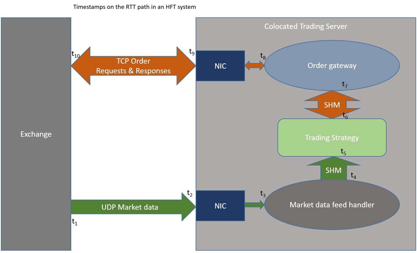
Figure 7.2 – Hops on the round trip path from the exchange to a participant and back to the exchange

The following table describes the different timestamps on the round trip path in greater detail. This outlines the different hopes when a single market data update generated from the exchange reaches a market participant and gets processed. On the path from the participant to the exchange, it describes the different hops for the order sent in reaction to the market update.

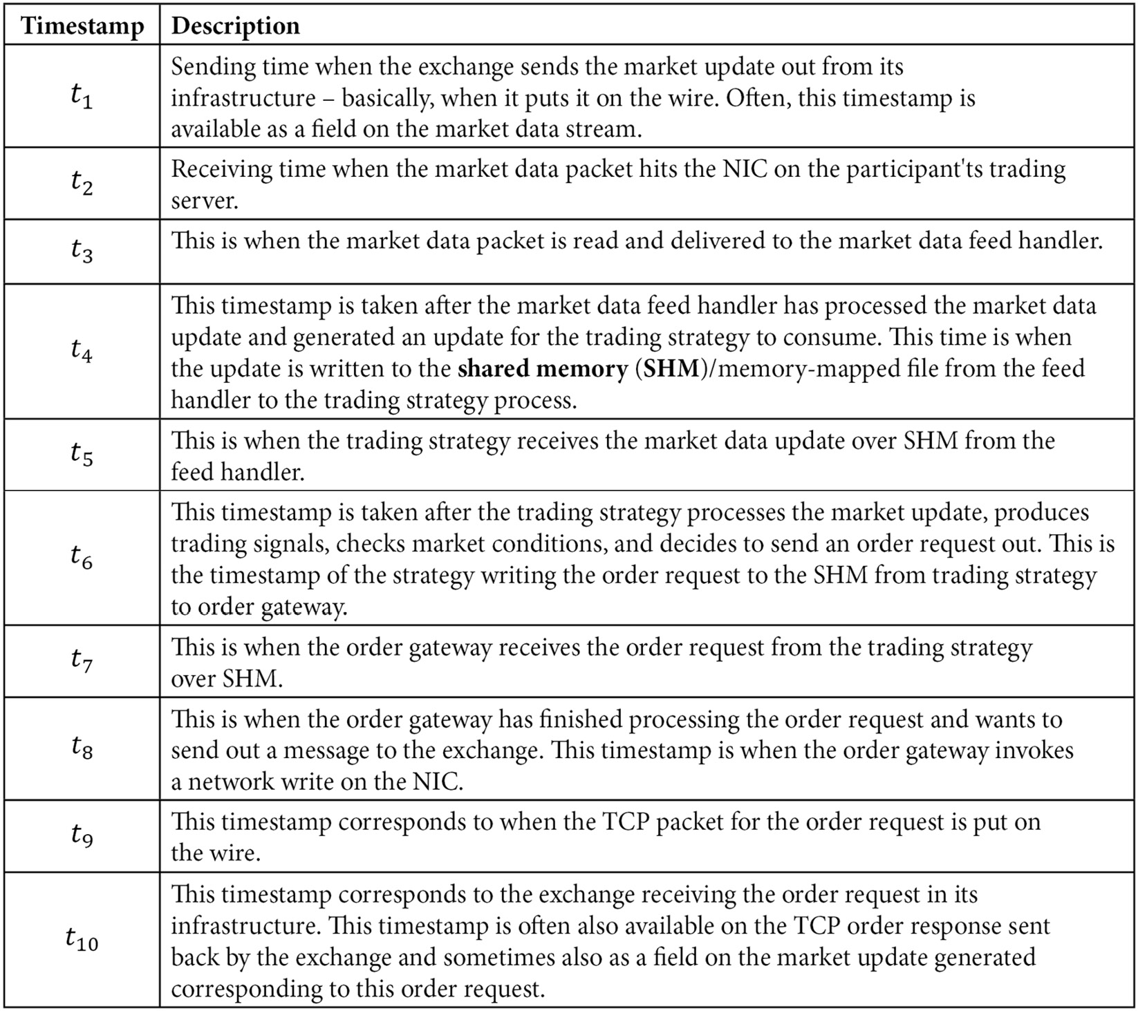
Figure 7.3 – Details of timestamps captured at different hops on the round trip path between the exchange and a market participant

This section described a typical end-to-end measurement system for an HFT ecosystem. We also investigated the different timestamps captured on the hops between market participants and the exchange in detail.

Summary

We discussed the implementation details of various computer science constructs, such as memory access mechanisms, network traffic access from the application layer, disk I/O, network transmission methods, and performance measurement tools and techniques.

We also discussed the implications that these features have on HFT applications and found that, often, the default behavior that works best for most applications is not the optimal setup for HFT applications.

Finally, we discussed approaches, tools, techniques, and optimizations for optimal HFT ecosystem performance. We hope this chapter provided insights into advanced HFT optimization techniques and their impact on the HFT ecosystem's performance.

You should have a good idea of all the important optimization considerations in an HFT ecosystem. We also discussed in great detail the different performance measurement and optimization tools and techniques you can use to profile the performance of your HFT system and maintain and improve on it.

In the next chapter, we will dive into modern C++ programming language details, specifically with the goal of building super-low-latency HFT systems that use all the power that modern C++ has to offer.