Chapter 9: Java and JVM for Low-Latency Systems

When people think about high-frequency trading (HFT), Java does not often come to mind. The Java virtual machine (JVM) warm-up, the fact that it is running on a virtual machine, and the infamous garbage collector have been big deterrents for programmers. However, if you smartly understand those limitations and code, Java can be used in a low-latency environment. You will then be able to benefit from all the advantages that come with Java:

• A very active and deep offering of free third-party libraries.
• Write it once, and compile and run it everywhere.
• Greater stability, avoiding the infamous segmentation fault due to bad memory management.

In this chapter, you will learn how to tune Java for HFT. The performance at runtime is largely based on the performance of the JVM. We will explain in depth how to optimize this critical component.

We will cover the following topics:

• Garbage collection
• JVM warm-up
• Measuring performance in Java
• Java threading
• High-performance data structures
• Logging and Database (DB) access

  Important Note

  In order to guide you through all the optimizations, you can refer to the following list of icons that represent a group of optimizations lowering the latency by a specific number of microseconds:

  : Lower than 20 microseconds

  : Lower than 5 microseconds

  : Lower than 500 nanoseconds

  You will find these icons in the headings of this chapter.

Before getting into the optimization, we would like to remind you how Java works. In the next section, we will describe the basics of Java.

Introducing the basics of Java

Java was created by Sun Microsystems in 1991. The first public version was released 5 years later. The main purpose of Java was to be portable and highly performant in internet applications. Unlike C++, Java is platform independent. The JVM ensures any architecture and operating system's portability.

Figure 9.1 shows the compilation chain for Java. We can observe that the Java compiler doesn't produce an executable but a bytecode. JVM will run this bytecode to run the software.

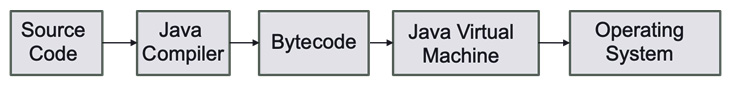
Figure 9.1 – Java compilation chain

We recommend reading the Packt book Java Programming for Beginners, written by Mark Lassof, to learn the characteristics of this language in detail. In this chapter, we will talk about the factors that will affect the performance of HFT. As we described for C++, one critical component is the memory management structure. Unlike C++, where the developer must handle memory manually, Java has a garbage collector (GC). The main purpose of the GC is to free objects (memory segments) from the heap when these objects are not used anymore.

Figure 9.2 describes how the memory is divided into different functional parts. The heap area is created when the JVM starts. To improve the data structures, objects at runtime are added to the heap area. In the section on the GC, we will see how to resize the heap to improve the performance at runtime. Like the heap, the method area is created at startup and stores class structures and methods.

Figure 9.2 – JVM memory area parts

When we create a thread, the JVM stack is used. This part of memory is used to store data temporarily. Native stack and PC registers are also created when the JVM starts but will not be a critical component for performance in HFT.

The component that is critical for performance is the GC. JVM triggers the garbage collection to automatically deallocate the memory of objects that are not used anymore in the heap.

Figure 9.3 represents the organization of the Java heap memory. The garbage collection will manage the object allocation on this part of the memory.

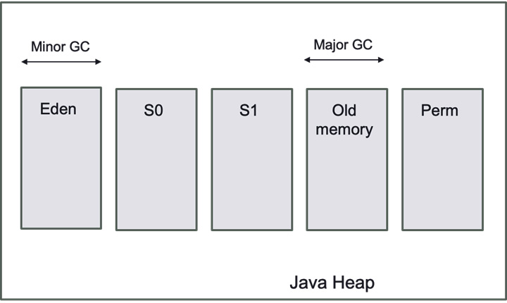
Figure 9.3 – JVM heap memory model

The two main parts to remember for HFT are Eden and old memory. When we create new objects, they go to the Eden part, while the objects remaining for the longest time will stay in the old memory. Allocating and deallocating objects takes time; that's why the garbage collection will be the main performance component in HFT.

We will now talk about garbage collection.

Reducing the impact of the GC

When Java was released in 1996, one of the big promises was the end of the dreadful segFault error, so familiar to all C/C++ developers. Java decided to remove all the objects and pointer life cycle out of the hands of the developer and entrust the logic to the JVM. This gave birth to the GC.

There is not a single type of garbage collection. There have been multiple versions developed; all have different specifications to offer either low-latency pauses, predictability, or high throughput.

One of the biggest parts of tuning Java is to find the most appropriate GC for your application as well as the best parameters for it. The main GC algorithms are as follows:

• Serial GC: Recommended for the small dataset or single-threaded with no pause time requirements.
• Parallel/throughput collector: Recommended for peak performance and not pause time requirements.
• Concurrent Mark Sweep collector: Recommended for minimum GC pause time.
• G1 GC: Recommended for minimum GC pause time.
• Shenandoah collector: Improved version of G1 GC, where pause time is no more proportional to the heap size. You can find more information here: https://wiki.openjdk.java.net/display/shenandoah.
• Z GC (Experimental): Recommended for high response time, very large heap, and small pause time. You can find more information here: https://wiki.openjdk.java.net/display/zgc/Main.
• Epsilon GC (Experimental): For the bold and brave, this is known as Java's no-op GC. It has the lowest number of GC interventions possible with no memory reclamation. It is recommended for people that understand the complete life cycle of objects created in their application.

It is beyond the scope of this book to exactly recommend a specific GC. If you would like to have more information, we recommend Packt's Garbage Collection Algorithms by Dmitry Soshnikov (https://www.packtpub.com/product/garbage-collection-algorithms/9781801074629). In a high-frequency environment, the less often and the less time we spend in the GC state, the better. That is why we will prefer using concurrent algorithms such as Concurrent Mark Sweep, G1, Shenandoah, and Z.

The only way to choose the best GC for your needs is to try all of them. It is important to measure performance to establish which algorithms will work the best. When testing performance, we want to enable the different GCs and run in an environment as close as the one running in production. Each GC algorithm also comes with a multitude of options that will allow you to control and tweak its behavior. There are no options that are better than the others; you will need to experiment to find the ones that have the best results for your application. We will find the right balance between the frequency and the duration of the GC. Do you prefer GC for 2 ms every 30 minutes or 4 ms every 60 minutes? These are questions you will need to answer. For a more in-depth look at the different GC algorithms and options, you can refer to the latest documentation on the Oracle website: https://docs.oracle.com/en/java/javase/18/gctuning/index.html.

We will now look at how we can limit the GC events as much as we can.

What to do to keep GC events low and fast

In HFT, we want to limit the effect of the GC. When a GC is triggered, it is difficult to keep control of the execution. The performance can be impacted whenever the GC is triggered. Therefore, it is important to keep the number of GC interventions low, and when the intervention is inevitable, we need to make it fast. The best way to reduce the number and the duration of the GC depends on the coding style. The more objects you create, the more pressure you are going to put on the GC. It is important to keep in mind that the creation of an object on the critical path may end up in the removal of this object at some point. The key is to pre-allocate objects that will live during the entire execution of the software to avoid allocation/deallocation triggering the work of the GC. Your primary goal is to avoid the frequent creation of short-lived objects.

You first need to identify the hot paths (functions or pieces of code that are constantly called at a very high frequency) in your program; once identified, you need to look for all the object creations in that path. If you know you will be creating thousands of objects for a very short time span, you will need to consider adding these objects to a cache pool. They will be first allocated and will be used afterward. Ideally, the hot path is single-threaded and spinning on a specific core (as we explained in the Reducing the number of contexts switched section in Chapter 6, HFT Optimization – Architecture and Operating System. This design will remove the need for any locks on the pool, and a simple counter to get and return the object will be enough. In some situations, even if it is multithreaded, it might still be good to use a pool even though you will need a lock. We can offset the cost of using a lock with a smaller GC time. By caching, we will increase the heap size. It is important to consider the tradeoff between the number of objects created with the heap size.

We will continue this section by talking about other Java features increasing the number of objects allocated that can potentially trigger the use of the JVM.

Limiting the autoboxing effect

Another critical coding style to pay attention to is autoboxing. Moving back and forth between a primary type and its object wrapper will create a lot of unnecessary objects. When the compiler automatically converts the primitive types into their corresponding Java object wrapper, it is called autoboxing. For example, converting int to an Integer, double to a Double, and so on. Inboxing is when the conversion goes the other way. Even though some wrappers contain a cache, it is relatively small. For example, for Integer, it only caches values between -127 and 127. If you need to use a wrapper, it is recommended to use Integer, because it is the only wrapper that allows you to extend the cache (-XX:AutoBoxCacheMax).

By default, Java offers a multitude of Collection, List, and Set implementations that will solve most of your needs. Unfortunately, all those structures only support objects as parameters, and most of them are also creating new objects on each insert in order to implement the desired behavior. When coding, you need to keep this in mind. You can also use some third-party libraries (https://fastutil.di.unimi.it/ or https://github.com/real-logic/agrona) that will implement the Java collection using the Java primary type. Depending on your needs this could greatly reduce the object creation in your program.

You also need to be mindful of the different objects that are created by either the code 's Java classes or any third-party libraries. You need to be aware of the object creations of which the Iterator is a perfect example. It will create a new object each time you call it. This is why you might give preference to a structure that supports a simple loop for each iteration. Another example is the libraries used to connect to databases. They are very dynamic but they could create a ton of objects on each insert.

The GC may be tweaked to reduce latency while increasing memory usage. After Oracle Java 11, the Epsilon option appeared. This option sets a GC that manages memory allocation but doesn't implement a memory reclamation mechanism. The JVM will shut down whenever the available Java heap is depleted. At the price of memory footprint and speed, this Epsilon provides a passive GC approach with a defined allocation limit and the lowest possible latency overhead. However, introducing manual memory management features in the Java language was not a goal.

Stop-the-world pause

In general, GC does not necessitate a stop-the-world (STW) pause. It means all the active threads pause and only the memory cleaner thread is running. It is called a stop-the-world pause because during that time, your program is not actively running. There are JVM implementations that do not have any pauses. Azul Zing JVM is one of them. The algorithm it employs determines whether or not JVM needs STW to collect trash.

Mark Sweep Compact (MSC) is a standard algorithm that is used by default in hot spots (a critical part of a code). It contains three steps and is implemented in an STW fashion:

• Mark: Traverses the live object graph to mark things that are accessible
• Sweep: Searches memory for unmarked memories
• Compact: Defragments memory by moving designated things

The JVM should fix all references to this object when shifting items in a heap. The object graph is inconsistent throughout the relocation process, so a STW pause is essential. An object graph is a list reporting the relationship between the different objects created. It allows them to know which objects are still needed and which ones are not referred to by any other and are free to be collected.

Concurrent Mark Sweep (CMS) is a HotSpot JVM technique that does not need the STW pause to gather old space (not the same thing as a full collection).

CMS does not use Compact and instead uses a write barrier (the trigger that acts each time you write a reference in the Java heap) to construct a concurrent version of Mark. Lack of compaction can cause fragmentation, and if background trash collection is not quick enough, the program may be halted. CMS will resort to STW MSC collection in certain circumstances.

We will now talk about how the Java primitive types can improve the garbage collection.

Primitive types and memory allocation

In addition to the previous methods to reduce the GC intervention, we can consider optimizing memory allocations. When primitive types are available, one technique to minimize latency is to employ them. Primitive types (often called primitives) use less memory than their object equivalents, which has the following benefits:

• It allows fitting more data into a single cache line. If the data the processor needs is not in the current cache line, a new 64-byte cache line will be loaded. If the CPU cannot anticipate the memory access, the retrieval operation might take 10 to 30 nanoseconds.
• If we can utilize less memory, we can keep the maximum heap size short, which means the collector has fewer live roots to search while doing a full GC with a lesser number of objects. A complete GC can easily take 1 second/gigabyte.
• Primitives decrease the amount of waste generated by a program. Most of the items you make will need to be gathered at some point. A minor GC is very quick at disposing of dead items; in fact, disposing of dead objects takes essentially no time at all because only living things are moved between (and into) the surviving areas; nonetheless, copying the live objects uses resources that may be utilized to conduct business logic.
• Assigning to a primitive is faster than generating a new object on the heap. Object creation in Java is extraordinarily fast, even faster than malloc in C, identifying a suitable portion of the main memory. The object is constructed in Java in the next accessible spot in a pre-existing buffer, referred to as the Eden space.
• Many functions return double values rather than a single number when building a pricing system. In a perfect world, objects would be preferred; however, this is not feasible because our computations occasionally fail, and we must produce an error or status code. If we need to return an object, in some cases, it could be re-used, so we could just pass it in the function as an argument.

We saw how primitives can help optimize the garbage collection; we will now talk about the profiling of memory.

Memory profiling

We talked about how to keep object creation to a minimum, but how do you keep track of the number of objects created by your program? The best way to do this is to use a Java profiler. There are many solutions (licensed or free) available:

• Profiler (https://www.ej-technologies.com/products/jprofiler/overview.html)
• Java Profiler: https://www.yourkit.com/java/profiler
• Visual VM: https://visualvm.github.io
• Apache NetBeans – Java profiler: https://netbeans.apache.org/kb/docs/java/profiler-intro.html

These software will give reports and graphs; they will be the primary visual evidence of a performance problem. Some will report the hotspots where most of the objects are created. They also incorporate performance measurement tools that could be helpful to find inefficiencies in your code. It is not recommended to use profiling software in a production environment. These tools are intrusive in terms of performance. They should run in a simulation environment, where we can recreate a mock of the production environment to make sure we explore all the paths in our code. We do not have to pound it with tons of data; profiling is not made to find what your system can handle, but how efficient it is with the resources.

Figure 9.4 represents the output of a Java profiler. We can actually see with the bars which part of the code is most time-consuming.

Figure 9.4 – Example of a Java profiler result

In this section, we talked in depth about the GC and its impact on performance. We saw how to limit its intervention by using coding techniques. We will now talk about the JVM warm-up, which is required to have performant code.

Warming up the JVM

Compileable languages, such as C++, are so named because the provided code is entirely binary and can be executed directly on the CPU. Because the interpreter (loaded on the destination machine) compiles each line of code as it runs, Python and Perl are referred to as interpreted languages. In Figure 9.1, we showed that Java is in the middle; it compiles the code into Java bytecode, which can then be turned into binary when necessary.

It's for long-term performance optimization that Java doesn't compile the code upon startup. Java builds frequently called code by watching the program run and analyzing real-time method invocations and class initializations. It might even make some educated guesses based on past experience. As a result, the compiled code is extremely quick. The main caveat for having an optimal execution time is to call the function many times.

Before a method can be optimized and compiled, it must be called a particular number of times to exceed the compilation threshold (the limit is configurable but typically around 10,000 calls). Unoptimized code will not run at full speed until then. There is a trade-off between getting a faster compilation and getting a better compilation (if the assumptions that the compiler takes in terms of execution were wrong, there would be a cost of recompilation).

We're back to square one when the Java application restarts, and we'll have to wait till we reach that threshold again. The HFT software has infrequent but crucial methods that are only called a few times but must be incredibly quick when they are.

Azul Zing solves these problems by allowing the JVM to store the state of compiled methods and classes in a profile. This one-of-a-kind feature, known as ReadyNow!®, ensures that Java programs always execute at maximum performance, even after a restart. You can find more information on ReadyNow on this website: https://www.azul.com/products/components/readynow.

When we resume a software (such as a trading system) with an existing profile, the Azul JVM remembers its prior decisions and compiles the described methods directly, which eliminates the Java warm-up problem.

We can also create a profile in a development environment to simulate production behavior. After that, the optimized profile can be deployed in production with the assurance that all key pathways have been compiled and optimized.

GraalVM recently also developed an ahead-of-time (AOT) project. We will not dive into the details, but it would allow you to pre-compile your binary code into native code. This would allow you to speed up the process at startup as the AOT native code would be used right away and until the tiered compilation kicked in. It was introduced in Java 9 as an experimental function. We will now explain how JVM optimizes the runtime using tiered compilation.

Tiered compilation in JVM

At runtime, the JVM understands and executes bytecode. In addition, just-in-time (JIT) compilation is used to improve performance. We had to manually pick between the two types of JIT compilers accessible in the HotSpot JVM in older versions of Java. One (C1) was designed to speed up application startup, while the other (C2) improved overall performance.

In order to attain the best of both worlds, Java 7 introduced layered compilation. For the most used parts, a JIT compiler converts bytecode to native code. HotSpot JVM gets its name from these parts, which are referred to as hotspots. As a result, Java may achieve performance comparable to a fully compiled language. There are two types of JIT compiler:

• C1 (client compiler), which optimizes the start-up time
• C2 (server compiler) is tuned for overall performance

In comparison to C1, C2 watches and analyzes the code for a longer length of time. This enables C2 to improve the compiled code's optimizations.

Compiling the same functions using the C2 compiler takes longer and uses more memory. However, it creates native code that is more optimized than C1. Java 7 was the first to introduce the idea of tiered compilation. Its objective was to achieve both rapid startup and strong long-term performance by combining C1 and C2 compilers.

Figure 9.5 shows the tiered compilation in JVM. When an application is first started, the JVM interprets all bytecode and accumulates profiling data. The acquired profiling information is then used by the JIT compiler to locate hotspots. To achieve native code speed, the JIT compiler first compiles the frequently performed parts of code using C1. When more profile data becomes available, C2 takes over. C2 recompiles the code using a more aggressive optimization algorithm.

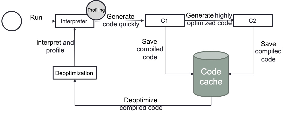
Figure 9.5 – Tiered compilation in JVM

Despite the fact that the JVM only has one interpreter and two JIT compilers, there are five layers of compilation, as shown in Figure 9.6. The reason is that the C1 compiler has three levels of operation. The quantity of profiling done is the difference between those three tiers.

Figure 9.6 – Compilation levels

We are going to describe the JVM compilation levels more in depth.

Level 0 – Interpreted code

The JVM understands all Java code the first time the code is run. When compared to compiled languages, performance is typically worse at this phase. However, following the warm-up phase, the JIT compiler kicks in and compiles the hot code at runtime. The profiling information gathered at this stage is used by the JIT compiler to conduct optimizations.

Level 1 – Simple C1 compiled code

The JVM compiles the code using the C1 compiler at this level, but without gathering any profiling data. For functions that are considered trivial (such as arithmetic operations), the JVM employs the compilation level 1. The C2 compilation would not make it quicker due to the minimal method complexity. As a result, the JVM believes that gathering profiling data for code that cannot be further optimized is pointless.

Level 2 – Limited C1 compiled code

At level 2, the JVM uses the C1 compiler with mild profiling to compile the code. When the C2 queue is full, the JVM switches to this level. To boost performance, the objective is to compile the code as fast as feasible. The JVM then recompiles the code on level 3 with full profiling afterward. Finally, the JVM recompiles the C2 queue on level 4 once it is less crowded.

Level 3 – Full C1 compiled code

At level 3, the JVM compiles the code with complete profiling using the C1 compiler. Level 3 is included in the standard compilation process. As a result, except for basic operations or when compiler queues are full, the JVM utilizes this level of compilation in all circumstances. In JIT compilation, the most typical case is that the interpreted code goes straight from level 0 to level 3.

Level 4 – C2 compiled code

On this level, the JVM uses the C2 compiler to build the code for the best long-term performance. Level 4 is likewise included in the standard compilation process. Except for simple methods, the JVM compiles all methods at this level. The JVM stops gathering profiling information because level 4 code is considered completely optimized. It may, however, decide to deoptimize the code and return it to level 0.

To summarize, the JVM interprets the code until a method reaches Tier3CompileThreshold. The method is then compiled using the C1 compiler, while profiling data is still being gathered. When the method's invocations reach Tier4CompileThreshold, the JVM compiles it using the C2 compiler. The JVM may eventually decide to deoptimize C2 compiled code. That implies the entire procedure will be repeated.

Each compilation threshold is associated with number of iterations. To find out the default value we can ask the JVM to print them using -XX:+PrintFlagsFinal:

intx CompileThreshold = 10000

intx Tier2CompileThreshold = 0

intx Tier3CompileThreshold = 2000

intx Tier4CompileThreshold = 15000

You can change those values using the JVM options if you want to lower or increase them. There is no magic number, each program is unique, so it is best to monitor the performance using different parameter combinations and choose the one that best satisfies your performance requirements.

We will now show how to optimize the JVM as soon as we start the software.

Optimizing the JVM for better startup performance

In HFT, we don't want to be able to get the best performance as soon as we run the software. We will explain the different methods we can use to avoid intermediate compilation.

Tiered compilation

We can run the JVM with the -XX:-Tiered Compilation option. It disables intermediate compilation tiers (1, 2, and 3) so that a method is either interpreted or compiled at the maximum optimization level (C2):

• ReservedCodeCacheSize:

The -XX:ReservedCodeCacheSize=N option specifies the maximum size of the code cache. The code cache is controlled in the same way as the rest of the JVM's memory: it has an initial size (given by -XX:InitialCodeCacheSize=N). The initial size of the code cache is allocated, and when the cache fills up, the size is increased. The code cache's initial size is determined by the architecture. This setting is useful because it has a small impact on speed.

• CompileThreshold:

The value of the -XX:CompileThreshold=N option triggers standard compilation. Java can run in client or server mode, and the default value will depend on that mode; it is 1,500 for client applications and 10,000 for server applications. Lowering this number could speed up the compilation to native code. It needs to be tuned based on the needs of each application; pick a number too small and the JVM will generate native code with limited profiling information and maybe not create the most optimized code for the long term. The threshold is determined by adding the total of the back-edge loop counter and the method entrance counter, despite the fact that there is only one flag here.

• Warm up your code:

You could write your own code warmer. As you are aware of the hot path in your program, you could write a wrapper that would execute that hot path in order to reach the minimum number of iterations for bytecode optimization. In an HFT system, the market data process is usually not an issue as you will very quickly reach the iteration threshold with the sheer amount of data you will receive. You should focus on the less frequent events such as new orders or execution of code that are called periodically, but you do not want to have them slow down your hot path. You need to be extremely careful about JVM warm-up in a live environment. To warm up the JVM, we can utilize a variety of techniques. The Java Microbenchmark Harness (JMH) is a toolkit that assists us in appropriately implementing Java microbenchmarks. For HFT, it could be a function on the critical path, such as the function in charge of sending orders. Once loaded, it continually executes a code snippet while keeping track of the warm-up iteration cycle. JMH was created by the same team that created the JVM. You can read about it here for your reference: https://www.baeldung.com/java-jvm-warmup.

The quickest approach to get started with JMH is to use the JMH Maven prototype to create a new JMH project. We will dive more into the details of JMH in the following section.

Measuring the performance of a Java software

JMH is a toolkit that assists you in appropriately implementing Java microbenchmarks. Let's now discuss them in detail.

Why are Java microbenchmarks difficult to create?

It's difficult to create benchmarks that accurately assess the performance of a tiny area of a bigger program. When the benchmark runs your component in isolation, the JVM or underlying hardware may apply a variety of optimizations to it. When the component is operating as part of a bigger application, certain optimizations may not be available. As a result, poorly designed microbenchmarks may lead you to assume that your component's performance is better than it actually is.

Writing a good Java microbenchmark often requires avoiding JVM and hardware optimizations that would not have been done in a genuine production system during microbenchmark execution. That's exactly what it is about. Benchmarks that correctly measure the performance of a tiny part of a larger application are challenging to come up with.

We are not going to dive into the details of how to implement JMH. There are multitudes of very good sources already available over the web. A must-read is the JMH GitHub (https://github.com/openjdk/jmh), which will provide you with instructions on how to install JMH but also has a multitude of examples. The JMH framework helps to reduce the warm-up period of an application. It could also be used to measure offline performances; it will help you in your design decisions. If you are hesitating between multiple design options or thinking about some optimizations, JMH can help you evaluate the performance and help confirm your choices. As we said a few times in this book, the key to optimization is to be sure that we measure the performance accurately to ensure that the optimization works. We will now talk about how to measure real-time performance.

Real-time performance measures

Harness testing will only allow you to make a decision on what is the best design to achieve the best throughput or speed. Once your code is released in a production environment, you need to keep track of the performance of the critical parts of your application.

A good measure that will not give you a pure performance report, but will let you spot quite easily changes in performance behavior, is to keep a revolutions per minute (RPM) on your hot threads. In an HFT application, you always have one or multiple threads that will be spinning on a core. You could keep a simple counter that will increment on each spin. If for any reason you have some code in that loop that starts misbehaving and it starts to add some drag, you will be able to detect it by observing a change in the RPM behavior.

The next measure to keep is latency. You want to keep simple latency measures in the critical part of your code, and if you have a distributed system, you also want to measure the communication latency between the different processes.

We need to be smart about collecting the latency and the RPM statistics. The last thing we want is to create more overhead and latency than in your standalone code when capturing statistics.

For this reason, the statistics collector should have very light and basic logic. There must be no lock or object creation at any time in the logic. You should have cumulative, incremental, and descriptive (min, max, avg, and pctXX) statistic collectors, as they will cover most of your needs.

Here are the different types of counters that we can use:

• Cumulative is an easy counter that could be incremented by any values.
• Incremental is a simple counter that can only be incremented by one.
• Descriptive keeps track of the minimum, maximum, average, and percentile X over the collection period.

You now need to collect the statistics for the period and store them to be able to analyze them. The best course of action is to have a periodic thread that awakens every X minutes (1 minute is a good number) that will grab and reset the statistics from all the collectors. It will then store the statistics to be able to visualize or analyze them. The storing must also be made in a smart way. Speed is not critical but object creation is; logs or database storage will generate a lot of object creations. A good solution is to send those statistics to a different process through either Inter-Processing Communication (IPC) or the User Datagram Protocol (UDP) and let the remote process take care of the storing. It is easy to send data to a remote process without creating any lock or object.

On the remote server, you are now free to use any software to store statistics and access the data easily, including databases and time-series data (for example, Graphite: https://grafana.com/oss/graphite/).

To visualize the stored data, a good option is the Grafana dashboard (https://grafana.com/grafana/). It is a frontend that can be linked to multiple data sources using different plugins. It will let you access those statistics through a nice website with lots of graph options and alert triggers. The raw data will be available on the box where Grafana is running or through a web API. The next section will talk about the performance that we can achieve with threading.

Java threading

Threads are the basic unit of concurrency in Java. Threads provide the advantage of reducing program execution time by allowing your program to either execute multiple tasks in parallel or execute on one portion of the job while another waits for something to happen (typically input/output (I/O)).

HFT architecture heavily uses threads to increase the throughput, as we mentioned in Chapter 7, HFT Optimization – Logging, Performance, and Networking. Multiple threads are created to do tasks in parallel. Adding threads to a program that is completely CPU bound can only slow it down. Adding threads may assist if it's totally or partially I/O bound, but there's a trade-off to consider between the overhead of adding threads and the increased work that will be done. We know that the underlying hardware (CPU and memory resource) will limit this throughput. If we increase the number of threads beyond a certain limit (such as the number of cores or the number of threading units), we deteriorate the performance by increasing the memory footprint (potentially decreasing the cache usage) or by increasing the number of context switches. If we notice that the latency of our trading system has been impacted and the memory usage has sharply increased, monitoring the number of threads will be required.

As we explained in Chapter 8, C++ – The Quest for Microsecond Latency, the rule of thumb to optimize HFT software is to be aware of bottlenecks. For instance, if an algorithm is susceptible to cache contention between multiple CPUs, it has the ability to wreak havoc on the thread's performance. When employing many CPUs to run a highly parallelized algorithm, cache contention is a critical consideration. There is no magic number for thread count; the goal is to minimize them while achieving the best throughput.

The use of a Java profiler will show the number of threads and list the GC threads that will be used within the trading system. This graphical tool has many features that could be useful to find objects or data structure being the contention of the tasks accomplished by the threads (finding bottlenecks). When using this tool, it is important to keep in mind that any profiler can be intrusive. There are simpler alternatives to query the number of threads in an application; for a Linux-based operating system (OS), the best one is htop (https://htop.dev/). It will give you an immediate view of how many threads are running within your Java process. For a Linux-based OS and other useful command-line tools, sending a kill –3 pid command will force the JVM to dump a list of all the threads in your program as well as what they are executing at the time of the call. This is a useful tool to use to diagnose blocked threads or unexpected behaviors.

Using a thread pool/queue with threads

Threads in Java are mapped to system-level threads, which are the resources of the OS. Creating too many threads can impact the performance, reduce the cache efficiency, and we can run out of these resources quickly. Because the OS will handle the scheduling of these threads, it is easy to conclude that these threads will have less time to do actual work.

The goal of the thread pool is to help resources and contain the parallelism in a certain capacity. When using thread pools, we write concurrent code that will be called in parallel when submitting tasks. The thread pool will perform these tasks by re-using threads. We will not pay the thread creation cost and we will be able to limit the number of threads. Figure 9.7 represents code (a submitter) submitting tasks to a thread pool. The thread pool will handle these tasks. We can see that the number of threads is important since it will increase the concurrent executions of these tasks:

Figure 9.7 – Tasks with a thread pool

It is a good practice to keep two distinct pools of threads: a smaller one in charge of running the short-lived task, and a bigger one for the long tasks (I/O access, DB, and logging, for example), the one that could take multiple seconds or even used in a forever-spinning loop.

There is also the concept of the scheduler in Java, where you can schedule a task to run at a specific time or at a constant interval. The scheduler usually runs on its own thread, and when triggered, delivers the task to the thread pool. It is helpful when you add your task to the scheduler to designate the pool it should be assigned to. You could also designate the tasks that will take a couple of microseconds to run directly in the scheduler thread. A typical example would be a triggered task that adds an event in a lock-free event queue. There is no need to handle the add logic in an external intermediary thread.

We will now talk about the different types of executors that can help to create thread pools.

Executors, Executor, and ExecutorService

We will simplify the explanation of the Executors by saying that they contain methods to create preconfigured thread pool instances. We use them to work with different thread pool implementations in Java. The ExecutorService interface includes a significant number of ways for controlling task progress and managing service termination. We may submit tasks for execution and manage their execution using the returned Future instance using this interface.

Thread map

In an HFT system, there is always a hot path that logic should be bound to a specific looping thread, and that thread should be pinned to a core on the OS. If one thread is not enough to process the amount of data, we can start other spinning threads and assign to each of them a subset of the data to process. The spinning thread should never access blocking I/O or avoid any OS call or lock. OS calls could be blocked by other OS calls coming from other threads on the systems or the OS itself.

When it comes to thread affinity, we need to also be conscious of the CPU architecture: the number of cores, Non-Uniform Memory Access (NUMA) domain, and network card core binding. If threads need to communicate with each other or some other application over shared memory or network traffic, they should all be running on the same NUMA domain. When processes are running on the same NUMA domain, they are sharing the same memory cache and avoiding crossing NUMA boundaries, which will cost us more in terms of performance. We also want to isolate the core at the OS level, which will prevent the OS from scheduling any other process on the reserved core. On a Linux-based OS, this is done using the isolcpu functionality. It will exclude the designated cores to be accessed by the OS.

Utility threads (logging, timer, DB, and others) do not need to be bound to specific cores; they just need to make sure they will not be running on a core shared with the OS.

A very nice library to allow us to bind our Java thread to a specific core is found here: https://github.com/OpenHFT/Java-Thread-Affinity.

This library will allow you to pin threads to specific cores directly from Java. It is a pretty excellent tool with a simple API that will let you acquire a core when starting a thread. We have multiple options where you can ask for the next available core on the socket or lock a specific core number, or even pre-allocate a set of cores and have them assigned in the order of acquisition.

Let's see an example:

IRunnable command = new IRunnable() {

                    @Override

                    public void run() {

                             Affinity.acquireLock(true); // Acquire the next free lock from the preallocated list

           s_log.info("Cpu Lock:" + Affinity.getCpu());

        s_log.info("On Next Core The assignment of CPUs is
: " +         AffinityLock.dumpLocks());

                        while (true) {

                                   processInternalEvent();

                        }

                    }

                };

A Linux-based OS offers another alternative: we could use htop (please see the previous reference) to manually assign a core for each thread. This is not ideal as it is a manual process and we need to redo the mapping each time the process is restarted. The advantage of this solution is that the assignment of the core is not final, so you could move your thread around to a different core. It is also a quick way to test the performance improvement or changes that your application could achieve when you are binding a thread to a core.

Taskset (https://man7.org/linux/man-pages/man1/taskset.1.html) on a Linux-based OS can also be used to limit which cores the Java application-free threads will be allowed to run on. This will apply to the main thread and all Java threads that are not bound to a core.

In Figure 9.8, the diagram is the best-case scenario:

Figure 9.8 – Ideal scenario to execute a parallel program

We can run the entire program on one NUMA domain. If we start our Java application using tasket --cpu-list 6-8, the main starting thread and all non-bounded threads will be limited to run on CPU cores 6, 7, and 8, keeping them on the same NUMA domain.

In HFT, the principal component for performance is the data structure. We will now study which data structure we should use in Java to build an HFT system.

High-performance task queue

To achieve performance, any trading system must have processes and threads working in parallel. Processing many operations at the same time is a way to save time. The communication between processes is very challenging in terms of speed and complexity. As we saw in Chapter 6, HFT Optimization - Architecture and Operating System, it is easy to create a segment of shared memory and share data between them. As we know, there is a problem with the synchronization of the access to the data because shared memory doesn't have any synchronization mechanism. The temptation of using a lock is high but performance will be affected by this kind of object.

In this section, we are going to review the different Java data structures that we use in HFT. The first one is the simplest: the queue.

Queues

Queues generally have a write contention on the head and tail and have variable sizes. They are either full or empty but never operate on the middle ground where the number of writes is equivalent to the number of reads. They use locks to deal with the write contention. The lock can cause context switches in the kernel. Since any context switches save and load the local memory of a given process, the cache will lose the data. In order to use caching in the best way, we need to have one core writing. However, if two separate threads are writing, each core will invalidate the cache line of the other.

In Chapter 6, HFT Optimization - Architecture and Operating System, in the Using lock-free data structures section, we showed how lock-free data structures are the way to go for HFT. The circular buffer or ring buffer enables processes or threads to transfer data without any locks. We are going to talk first about the circular buffer.

Circular buffer

There are several names for a ring buffer. Circular buffers, circular queues, and cyclic buffers are all terms you've probably heard of. They all imply the same thing. It's essentially a linear data structure with the end pointing back to the beginning. It's simple to think of it as a circular array with no end.

A ring buffer, as you might expect, is mostly used as a queue. It has read and write positions, which the consumer and producer utilize separately. The read or write index is reset to 0 when it reaches the end of the underlying array. The problem comes when a reader is slower than a writer. We have two options: the first is to overwrite the data if we do not need the data anymore or to block the writer from writing (potentially having a write buffer).

The option to increase the size of a circular buffer is feasible. However, it must be done only if the read/write is blocked. In this situation, resizing will require moving all the elements to a newly allocated bigger array. This operation is very expensive and slow. It cannot be done on the critical path.

One of the implementations of the circular buffer is made by LMAX, and is called the LMAX disruptor.

LMAX disruptor

Disruptor uses a circular buffer. All events are broadcast (multicast) to all consumers for consumption concurrently via distinct downstream queues. Disruptors are similar to a multicast graph of queues in which producers send items to all consumers for concurrent consumption via distinct downstream queues. The consumer could be a chain of event handlers, allowing you to run multiple handlers for each consumed message. When we examine the network of queues more closely, we can see that it is actually a single data structure called a ring buffer. It is required to synchronize the dependencies between the consumers since they are all reading at the same time.

A sequence counter is used by producers and consumers to identify which slot in the buffer they are presently working on. Each producer/consumer can create their own sequence counters, but they may read the sequence counters of other producers/consumers. Producers and consumers check the counters to confirm that the slot they wish to write in is unlocked.

The disruptor is designed to address internal latency issues in Java processes. It is not a permanent store; messages remain in memory, and it is primarily intended to reduce latency between two or more worker threads serving as producers or consumers. It's faster than using ArrayBlockingQueue, which is Java's standard thread-safe class for this purpose. If we work with a high-throughput system that also has to ensure that each message is delivered as rapidly as feasible, this library becomes more appealing.

The disruptor is a lock-free data structure. The benefits are the same as the ones we described in Chapter 6, HFT Optimization – Architecture and Operating System, in the Using lock-free data structures section. In terms of Java, when compared to LinkedList, the disruptor ensures that elements are stored in a single contiguous block of memory and that elements are pre-fetched/loaded into the local CPU cache. Each logical item in memory is physically assigned to the next, and values are cached before they are needed. When compared to LinkedList, values are dispersed broadly across the heap memory when allocated, resulting in the loss of valuable CPU cache hits. A predetermined number of container objects are also pre-allocated in the ring buffer.

Because these containers are reference types or objects, they will reside on the heap, but they will be re-used once a buffer space is reclaimed. Because of this constant re-use, containers last indefinitely and are unaffected by the GC's STW pauses. To avoid indirectly allocating to the heap, we must remember that nested values on those objects are preserved as primitive values.

This section studied the LMAX disruptor; we will now review the conversant disruptor, another candidate for lock-free data structures.

Conversant disruptor

We will first talk about the design of a conversant disruptor. The underlying data structure of this disruptor is a ring buffer and a queue. The main advantage is to flush the entire queue as a batch using CAS comparison.

The conversant doesn't require any extract code; it is based on the Java BlockingQueue interface and is not domain-specific. It also works without the need for memory pre-allocation. The performance to push-pull an object in the multithreaded versions is 20 nanoseconds, whereas the push-pull variant takes 5 nanoseconds. This intrinsic quickness is primarily due to mechanical sympathy and simplicity. This implementation takes into account hardware specificities.

The conversant disruptor is different from the LMAX disruptor and is not a fork of the LMAX disruptor. They are essentially diverse in design and implementation, but they both have similar functionality. It makes sense to utilize the LMAX disruptor's implementation if we use the domain model. The conversant disruptor is the ideal choice for the typical use case of using a Java BlockingQueue interface as a fundamental data structure at the center of an application.

Agrona circular buffer

This is another available solution provided by the Agrona Project (https://aeroncookbook.com/agrona/concurrent/). Like the LMAX disruptor, it uses a specific interface, and we cannot simply swap classes that implement the Java queue interface with it. It offers one producer-one consumer (OneToOneRingBuffer), or many producers-one consumer (ManyToOneRingBuffer) solutions. It provides multiple options for the idle strategy, giving you more control over your reader and writer thread behavior. We reviewed the different lock-free data structures we can use in Java. We will now talk about the last part of this chapter, the logging and the DB access specific to Java programming.

Logging and DB access

As we explained in Chapter 7, HFT Optimization – Logging, Performance, and Networking, logging is critical for any trading system. It enables users to debug strategies, improve the return, compare theoretical and actual profit and loss, and store information in databases. It always requires a costly input/output. Therefore, logging cannot be done on the critical path. Like C++, a specific technique is needed to achieve performance in Java.

When creating a log, it can store trades in a database or build a string in a flat file. When generating a string to be pushed in the logging system, creating a string is a very time-consuming construction. It is essential to consider the speed of the system and the object's reaction. For instance, log4j zeroGC is a zero object creation logging framework, but it will generate the log message before putting it on the logger thread queue (in this case, the disruptor from LMAX). Your main application thread will need to generate the news, and this will have a cost on the performance. Nevertheless, this is still an acceptable solution for HFT systems.

You could develop your logging framework; we can still use the disruptor but store the unformatted log messages in the disruptor queue and then do the string creation in the consumer thread. You need to have objects added to the queue but writing the formatted logs into the appender can be done in a non-critical thread using a buffer without generating a string object.

We can find many frameworks, including java.util.logging, log4j, logback, and SLF4J. If we are building a microservice or another application with complete control over the execution environment, we oversee choosing a logging framework. Changing logging frameworks is usually as easy as searching and replacing, or in the worst-case scenario, a more complicated structural search and replace accessible in more powerful IDEs. If logging speed is crucial, which is the case in HFT, a logging API will always be better.

Choosing a framework will imply doing some benchmarking. When comparing the different frameworks, we need to keep in mind that the java.util.logging philosophy is that logging should be rare rather than the rule, while log4j 2.x and logback have a design for permanent logging.

Java util logging is less efficient than the logging API framework on the performance side because there is no buffer management, which affects logging speed significantly. The ability to buffer file I/O has the biggest influence on performance when configuring logging. The downside of activating buffer handling is the risk that the data is not pushed to disk if the process of writing this log fails. Another issue with buffering is that it might make it challenging to monitor the system in real time by tailing the log files. Buffering with a guaranteed maximum duration before flushing would be helpful if the various logging frameworks provided it. Having a flush every 100 ms would not have as large of an impact on system performance as flushing after each log statement, and it would allow humans to follow the log in real time.

Once we find the best logging infrastructure, we need to think about where to store the data. We can have a flat file or a database using the system logging framework.

We can review the advantages of these different media:

• file: Good for development and testing environments, but impacts the performance by the number of I/Os for the production environment. If the use of files is needed, we recommend a memory map file, which is blazing fast but not persisted.
• Database: Easy to retrieve and query but slow. The interaction with databases creates many objects. It might be better to send it on the wire (UDP or shared memory) and have an external process to do the logging. The downside is the need to ensure that the remote process keeps running.
• Syslog: Lets you send data on a UDP socket and is fast with low memory usage. We can configure Syslog in multiple ways. The logs can be kept locally or sent to a central server (https://github.com/syslog-ng/syslog-ng).

Let's see which process to choose for logging and database interactions.

External or internal thread?

When it comes to logging and database interactions, we have two choices: keep the logic in the main program using a dedicated thread or send the information to a reliable process using a straightforward and fast communication technique (UDP or shared memory).

If we choose to use logic in the main program, we add reliability, but we risk putting more pressure on the GC because of the object creations.

If we rely on a specialized external process, we risk sending information in an insecure way as we cannot guarantee that someone isn't listening on the other end. The benefit is that your main program does not need to worry about object creations coming from the logging or DB framework. We can send all the information from our main program as byte-encoded messages, which could be done with zero object creation. We are now free to code in the specialized node without worrying about having the GC kicking in too often. An excellent library to handle all the binary encoding can be found at https://github.com/real-logic/simple-binary-encoding.

For logging, fully encoding large messages could be too costly. A solution is to use a dictionary of the different messages assigned with numeric codes. When we want to send information to a specialized process, you encode the code and the values carrying the information. This can be done with zero objection creation and is amazingly fast. On the other hand, the specialized node is free to insert the data into the DB or recreate the string to log without having to worry about the pressure the object creation can have on the GC.

Summary

This chapter showed that JVM eases software developers' lives but impedes a trading system's performance. We demonstrated that by understanding how the JVM behaves under the hood, following good coding practice, and tuning the JVM, we could use Java as a serious programming language candidate for HFT. We studied in detail how to measure performance with Java. We know that measuring the execution time is the only evidence that code performs better after optimization. As we did with C++, we introduced high-performance data structures helping to get a performant code. We combined these data structures with the use of threads and thread pools. We concluded by discussing logging and database access, which are vital in HFT.

C++ and Java are the most used languages in HFT. The next chapter will talk about another programming language: Python. We will see how Python can be used in HFT and run fast using external libraries.