14

Signal Transforms

The idea of exploiting sampling randomization to achieve the capability of alias-free signal processing in a wide frequency range is attractive and often attracts attention. However, to achieve good results processing of nonuniformly represented signals must be carried out using special algorithms that take into account the specifics of this sampling approach. While this may seem to be obvious, it is less clear what criteria are required for evaluating the degree of matching the specifics of signal sampling and processing. This is not a trivial question. The following discussions explain to some extent why this is so. More about this is discussed in Chapter 18.

14.1 Problem of Matching Signal Processing to Sampling

These discussions will start by considering an example. Suppose that the mean power P_x of a wideband signal x(t) component at frequency ω_i that exceeds the mean sampling frequency ω_s has to be estimated. The application of random sampling is clearly indicated. At first glance it seems that this task can be solved by estimating the Fourier coefficients a_i and b_i at the frequency ω_i on the basis of the often applied formulae

The required estimate is then given as

Although these equations look like their conventional counterparts, they are in fact modified versions because the sample values of the signal and the functions cos ωt and sin ωt are taken irregularly and simultaneously at the random time instants {t_k}. This is done in an attempt to realize processing of the nonuniformly sampled signal in a proper manner. If the sampling operation is performed in accordance with the additive random point process, then, as shown in Chapter 6, the estimates are virtually unbiased and consequently they and the estimate _x contain only random errors.

Now the question may be asked as to whether the processing algorithm in this case is matched to sampling or not. On the one hand, the answer to this question could be affirmative: to some extent this estimation method is matched to the specifics of random sampling. The absence of the bias errors might be considered as evidence showing this to be the case. On the other hand, the answer to this question could just as well be negative. The degree of match between sampling and processing could be regarded as poor, first of all because the processing algorithm considered, which was initially developed for estimating the orthogonal signal components, in this case is applied to estimating signal components that after random sampling are no longer orthogonal. However, this fact is ignored.

The mutual unorthogonality of the randomly sampled functions sin ω_it_k and cos ω_it_k means that the estimation of one is influenced by the other. Moreover, these two randomly sampled functions are also nonorthogonal with regard to all of the other signal components. Consequently, the so-called random estimation errors in this case are not really random at all. They are actually caused, at least partly, by the interaction of all the signal components.

This sort of cross-interference between signal components is a basic phenomenon playing a significant negative role in processing of nonuniformly sampled signals. It must not be ignored. A particular approach to digital processing of signals that helps to get rid of this disadvantage is based on unorthogonal transforms. The mathematical apparatus of unorthogonal transforms is a powerful tool for dealing with many problems arising in advanced processing of irregularly sampled signals. Although many signal processing tasks may be reduced to unorthogonal transforms, application of them is effective only under certain conditions.

When the conditions for signal processing meet the requirements of correct unorthogonal transforms, the obtained results are really good. Then the distortions of the signal processing results due to the impact of sampling irregularities are taken out completely, which is demonstrated in this chapter. In other cases when it is not applicable, adapting signal processing to the specific nonuniformities of the sampling process might be attempted, as shown in Chapter 18.

14.2 Bases of Signal Transforms

Suppose that a signal, represented by the function x(t), can be given as

where φ_i(t) are functions from a system

Depending on the properties of the function system Φ, the coefficients {c_i} of the series (14.2) are obtained in different ways. The equations establishing the relationships between x(t) and the coefficients {c_i} of the respective system Φ define the corresponding signal transform.

The usefulness of such signal transforms is obvious. First of all, they can be applied to decompose the signals into their components, whose definition will depend on a priori information about signal properties and signal source. Solving most signal processing tasks, such as filtering, signal enhancement and extraction from noise, spectral analysis, identification and recognition, data compression and many others, involves some kind of signal transform and it can be shown that conventional orthogonal transforms do not always provide the best results.

14.2.1 Required Properties of the Transform Bases

The function system Φ is the basis of the corresponding signal transforms. There are certain requirements that it has to satisfy:

1. Completeness. A system Φ is considered to be complete for a certain space of functions if any function x(t) from this space can be represented by the series given by Equation (14.2).
2. Linear independence. All functions {φ_i(t)} of the system Φ should be linearly independent.

To prove this, consider the case when, for instance, φ_i(t) is linearly dependent on other functions of the corresponding system. Then

Substitution of Equation (14.4) into Equation (14.2) gives

which means that it is possible to express the function x(t) by all other functions of the corresponding system Φ without the function {φ_i(t)}. Hence this function, when it linearly depends on the other functions of the system Φ, is redundant.

It seems that no more than these two conditions have to be satisfied for a correct application of the signal transforms discussed here. The discussion of when and why the orthogonality of the basis functions is required follows.

14.2.2 Transforms by Means of a Finite Number of Basis Functions

According to Equation (14.2), the signal x(t) is in general represented by an infinite series. In practice, the number of terms of such a series is always finite. Therefore, it is more appropriate to talk about approximating the signal. To do this, the series

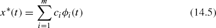
has to be constructed, so that x*(t) approximates x(t) sufficiently closely. The least squares approximation error can be used as a criterion for evaluating this closeness.

Now the approximation task both for analog and digital signals will be considered.

Analog Processing

The coefficients {c_i} for the series (14.5) can be determined by solving the following minimization task:

To find the minimum of the integral (14.6), all the individual derivatives of {c_j} should be considered as being equal to zero. Then

Therefore m linear equations are obtained, which can be incorporated into the following system:

This system of equations can be represented by

where

Solving the equation system (14.8) provides the coefficients {c_i}, . Obviously, the number of linearly independent functions of the system Φ = {φ₁(t), φ₂(t),..., φ_m(t)} is equal to the number of linearly independent equations of system (14.8).

Digital Processing

The above minimization task in this case is given by

which leads to the following equation system:

This system can also be represented by system (14.8), although in this case

A system of digital functions Φ = {φ(t), k = } cannot contain more than N linearly independent functions. To check this, assume that, contrary to this statement, the system Φ contains (N + 1) linearly independent functions. Express the (N + 1) th function φ_N+1(t_k) through the other functions as

where {d_i}, i = , are unknown variables. Each of the digital functions φ_i(t_k), k = , can be considered as an N-dimensional vector and the matrix of the equation system (14.15) represents these vectors in such a way that the ith column defines the ith vector φ_i(t_k), k = . According to the assumption all N vectors are linearly independent, the determinant of system (14.15) differs from zero and this equation system has only one solution. The kth equation of this system can be written as

which shows that the function φ_N+1(t_k), k = , represents a linear combination of the other N functions. As this contradicts the assumption, the initial statement is proved to be correct.

Thus, in the case of the discrete transforms, the number m of the functions of series (14.15) is limited by the number N of the signal sample values processed and the following unequality should be satisfied:

14.3 Orthogonal Transforms

The linearly independent functions of the system Φ = {φ₁(t), φ₂(t),..., φ_m(t)} are orthogonal if in the time interval [0, Θ] the following conditions are satisfied:

Denote √α_ii by ||φ_i(t)||. This parameter of the function φ_i(t) is considered to be its norm. If for all i

the corresponding system of functions is described as orthonormalized. In the case of digitized signals, conditions (14.17) become

Now consider solving the equation system (14.18) in the case when the basis functions are orthogonal. Then

and the equation system in question is reduced to the following system of equalities:

Thus we come to the conclusion that the orthogonal basis functions are a particular case of linearly independent basis functions and their application considerably simplifies the corresponding signal transforms. The coefficients {c_i} calculated in the course of the orthogonal transforms can be obtained directly without solving the equation system under consideration.

14.3.1 Analog Processing

It follows from Equations (14.10) and (14.20) that the coefficients {c_i} in the case of the orthogonal transforms are given as

where the norm

Note that in this case the number m of the approximation terms is unlimited, as long as the orthogonality conditions are satisfied.

14.3.2 Digital Processing

Similarly, it follows from Equations (14.14) and (14.20) that

where

The theory of discrete orthogonal transforms is well developed and their properties, with emphasis on the positive aspects, are well known. It can even be said that modern signal processing techniques are to a large extent founded on the concepts of discrete orthogonal transforms. They are so popular, and so widely discussed in numerous publications, that it is not necessary to discuss them here in detail. This category of transforms is considered first of all for the purpose of a survey to indicate the role of orthogonal transforms in the general scheme of signal transforms as a whole.

There can be no doubt that discrete orthogonal transforms have significant advantages. They can be carried out by performing relatively few multiplication and summing operations, and they are well suited to the application of so-called fast algorithms. On the other hand, discrete orthogonal transforms also have considerable drawbacks. The following are a few of these:

1. The orthogonal transforms of signals actually represent their approximations within a given time interval, and these approximations are not applicable for extrapolating or predicting the signals outside this interval.
2. When they are used, it is difficult, or sometimes impossible, to gain from a priori information about the input signal source or structure.
3. Orthogonal transforms do not allow signals to be decomposed into their true components if the latter are mutually unorthogonal.
4. This category of transforms is not applicable to irregularly sampled signals.

The last disadvantage calls for comment. Sometimes the fact that a signal has been sampled randomly or irregularly can be ignored and the orthogonal transforms can be applied. In this case additional estimation errors will result from sampling irregularities. If this is acceptable, irregularly sampled signals can be transformed in this way.

14.4 Discrete Unorthogonal Transforms

A signal transform is considered unorthogonal if the system of functions Φ = {φ_i(t_k), k = }, applied to perform the transform, is unorthogonal. It is agreed that the system Φ does not contain any functions identically equal to zero. Under this condition, ||φ_i(t)||² > 0 for all i = .

A few typical signal processing applications will now be mentioned where the signals need to be transformed on the basis of unorthogonal transforms:

1. Signal transforms carried out by means of a system of analog functions, which are originally orthogonal and become unorthogonal in the course of digitizing, as when the sampling applied is irregular. As an example to illustrate this case, refer to Chapter 15, where the discrete Fourier transforms of randomly sampled signals are discussed.
2. Short-time periodic signal spectrum analysis, when the signals have to be transformed under the condition that the observation time interval [0, Θ] is shorter than the given period of the signal. In this case the frequencies of the true signal components are known but the system of the functions {φ(t)}, chosen correspondingly, is unorthogonal.
3. Spectrum analysis of quasi-periodic signals, which are actually nonstationary with a slowly varying period.
4. Spectrum analysis of signals containing components at frequencies irregularly spaced along the frequency axis.
5. Decomposing signals into true components, which are mutually unorthogonal.

Even this incomplete list of unorthogonal transform applications shows that the problems approached in this way are significant. In this book, the most interest lies in the first application.

Now consider a system of functions Φ = {φ_i(t_k), k = }, i = , which is unorthogonal. Some nonzero coefficients α_ij, j ≠ i, which are not placed on the diagonal of the corresponding matrix defined by the equation system (14.12), definitely exist. For this reason, this equation system cannot be reduced to the system of equalities (14.20). Hence, the coefficients {c_i}, i = , have to be calculated on the basis of the equation system (14.12) and the condition (14.16) should be met.

The equation system (14.12) can be represented in the form of the following matrix equation:

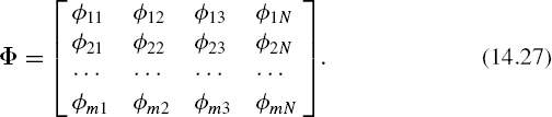
where the matrix

is square and contains (m × m) elements. It follows from definition (14.13) of its elements α_ji that this matrix is also symmetric. The vectors of the coefficients {c_i}, i = , and their estimates {c_i} are given by the respective columns

where the estimates {ĉ_i} are defined by Equation (14.14). It follows from Equation (14.23) that

where A⁻¹ is the inverse of matrix A.

It can be seen from Equation (14.14) that each estimate {ĉ_j} is obtained from a scalar multiplication of the vectors {x(t_k)} and {φ_j(t_k)}, k = . To obtain the coefficients themselves, the vector C according to Equation (14.25) should be multiplied by the matrix A⁻¹. Hence,

where α*_ji are elements of the matrix A⁻¹.

Thus, to carry out such unorthogonal transforms, all the elements of the matrix A should be determined while the estimates {ĉ_j} are being calculated; then the matrix A should be inverted in order to obtain the coefficients. As the inversion of such matrices is time consuming, this unorthogonal transform procedure is not suitable for real-time applications. Fortunately, it is often possible to compose the matrix A and invert it beforehand. Then the coefficients {ĉ_j} can be calculated much more quickly.

Such an approach can be applied when the unorthogonal transforms are performed in order to eliminate the errors due to sampling irregularities. If the sampling point process {t_k} is generated pseudo-randomly, all the functions of the system Φ are fully defined and the matrix A and its inverse can be obtained beforehand. Although in this case there are no problems and this method of performing unorthogonal transforms can be widely applied, it can still be improved, as the next section will show.

14.5 Conversion of Unorthogonal Transforms

Suppose that a signal is sampled pseudo-randomly and that the sampling point process {t_k} is fixed, Denote the values φ_j(t_k) by φ_ik. Then the system Φ of the given values can be written as

If the digital signal is represented as

it follows from Equation (14.14) that

Substitution of expression (14.28) into Equation (14.23) yields

Multiply both sides of this equation by the inverse matrix A. Then

where

It follows from Equation (14.30) that

where Φ^T is the transpose of matrix Φ. Hence

Substitution of this expression into Equation (14.30) yields

As A is a square m × m matrix, the inverse matrix A⁻¹ is also square and also contains m × m elements.

The matrix Φ, as can be seen from its definition (14.27), is a rectangular m × N matrix. Hence the matrix Ψ is also rectangular and contains m × N elements. This matrix can be given as

It follows from Equations (14.29) and (14.33) that

Equations (14.33) and (14.35) lead to the following conclusion. If the initial system Φ of the unorthogonal basis functions is replaced by the equivalent system Ψ, defined by Equation (14.33), the unorthogonal transforms can be calculated directly.

This method of performing the unorthogonal transforms is especially efficient under conditions where the functions {ψ(t_k)} can be calculated beforehand, so that the corresponding data can be stored in a memory. When the unorthogonal transforms are used for excluding the errors caused by sampling irregularities, these functions can be determined only for given particular realizations of the sampling point processes and, for this reason, it is convenient to use pseudo-random sampling.

Note that when the unorthogonal transforms are performed according to this approach, this method can be implemented by the same electronic devices that are commonly used for the DFT. The only difference is that when they are applied for calculating the unorthogonal transforms, the discrete values of {sin ω_it_k, cos ω_it_k}, which are kept stored in a memory unit, should be replaced by the sample values of the functions {ψ(t_k)}. Even the operational characteristics, like the number of operations per second and the accuracy of the results obtained, will be the same in both cases. The only disadvantage of performing the unorthogonal transforms in this way is that there are no fast algorithms for calculating them. At least, they have not yet been discovered.

Bibliography

Bilinskis, I. and Mikelsons, A. (1992) Randomized Signal Processing. Prentice-Hall International (UK) Ltd.