4
Randomized Quantization
Quantizing is usually defined as a rounding-off operation and this definition fits both the deterministic and the randomized versions of this operation. The quantization process is always carried out according to the same generalized scheme, given in Figure 4.1. To quantize a signal, instantaneous values are first roughly measured and then the measurement results are rounded off. The differences lie in how in these procedures are implemented, leading to various properties of the quantized signals. While the signal instantaneous values are always measured by comparing them with some reference threshold levels, the latter are kept in fixed positions for deterministic quantizing and are randomly varied for randomized quantizing. This means that the rounding-off function in both cases is carried out in two different ways. It is deterministic in the first case and probabilistic in the second case. Realization of the second approach seems to be and usually is more complicated than the first. However, under certain conditions it pays to perform quantizing of signals in this more complicated way as the properties of the quantized signals are quite different, which leads to various potential desirable benefits. On the other hand, the errors of randomized quantizing are typically distributed in an interval that is twice larger than those of comparable deterministic quantization. Essentials, advantages and drawbacks of this quantization approach are discussed in this chapter.
4.1 Randomized Versus Deterministic Quantization
Assume that the signals to be quantized are within the signal amplitude range [−Am, Am]. To perform B-bit quantizing, this range is subdivided into 2(2B−1 – 1) elementary intervals q, which are known as quantization steps. In the course of quantizing, the instantaneous values of signals have to be measured and rounded off, so the quantized signal is represented in the following form:

Figure 4.1 Essence of the quantizing operation
![]()
where
![]()
4.1.1 Basics
Everything said so far applies to both deterministic and the most popular versions of randomized quantizing. However, if the quantization operation is considered in some detail, then the deterministic and randomized quantizing of course differ. To continue this discussion, look at Figure 4.2, where the time diagrams illustrating deterministic quantizing of a unipolar signal are presented. The levels q, 2q, 3q, ..., to which input signal instantaneous values are rounded off, are shown in Figure 4.2(a) by dashed lines. They are in fixed positions. The distance between them is equal to the quantization step q.
To express the instantaneous values of the input signal in terms of q, they are first compared with another set of reference levels. In the case illustrated by Figure 4.2(a) these levels are constant. The distance between two of them is also equal to q, but the whole set of reference levels is located so that the first of them is elevated above the x axis by half the quantization step q. The measurement procedure is accomplished by comparing the signal with these reference levels and counting the number n of them that are below the signal's instantaneous value. When the signal being quantized is analog, as it is in the case shown, the quantized signal changes its value stepwise whenever the input signal crosses one of the reference thresholds. As can be seen from the diagrams, rough deterministic quantization is a typical nonlinear operation insensitive to small changes in the input signal.
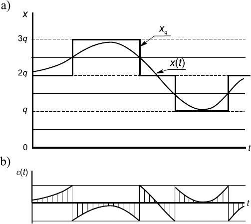
Figure 4.2 Time diagrams illustrating uniform deterministic quantizing: (a) original and quantized signals; (b) quantization noise
Randomized quantizing follows the same procedure, but in this case the reference levels are not fixed: they change continuously or step by random step from one quantizing instant to the next, as can be seen in Figure 4.3. Randomly (or pseudo-randomly) quantized signals are henceforth denoted by ![]() . The notation
. The notation ![]() is used because it is simple. However, it should be noted that
is used because it is simple. However, it should be noted that ![]() does not denote the estimate of the corresponding signal value, unlike other similar notations used in this book. Then
does not denote the estimate of the corresponding signal value, unlike other similar notations used in this book. Then
![]()
Formally, the rounded-off values of a randomly quantized signal are determined in the same way as for deterministic quantizing, i.e. the randomly changing threshold levels below the respective signal sample value are counted and the quantized signal ![]() k is defined as being equal to nkq. However, the essence of this roundingoff operation in the case of randomized quantizing is quite different. As explained further, for randomized quantizing this operation is probabilistic. This means that one and the same instantaneous value of a signal with probabilities depending on that signal value might be rounded off to various digital levels. As a result, the properties of a randomly quantized signal differ significantly from the properties of a deterministically quantized signal.
k is defined as being equal to nkq. However, the essence of this roundingoff operation in the case of randomized quantizing is quite different. As explained further, for randomized quantizing this operation is probabilistic. This means that one and the same instantaneous value of a signal with probabilities depending on that signal value might be rounded off to various digital levels. As a result, the properties of a randomly quantized signal differ significantly from the properties of a deterministically quantized signal.

Figure 4.3 Illustration of randomized quantizing
Note that there are two seemingly different approaches to randomization of quantizing. While in the quite popular cases of so-called dithering, mentioned in Chapter 1, noise is added to the signal at the input of a deterministic quantizer, the quantization operation could also be randomized as explained above by just forming time variable sets of reference levels and using them for rounding off the input signal instantaneous values. Electronic implementations of these randomized quantization schemes are indeed different. However, the essence of them is equivalent. It does not matter exactly how the randomness is introduced at quantizing. The results are exactly the same.
4.1.2 Input–Output Characteristics
The essentials of various quantization models can also be illustrated by specific representation of the quantized signals, including their input–output characteristics, shown in Figure 4.4. While deterministic quantization has one fixed input–output relationship (Figure 4.4(a)), randomized quantization, in general, is characterized by different input–output relationships depending on the specific quantizing model used. Moreover, the outcome of such quantizing, even for a specific quantizing model, is determined by instantaneous input–output characteristics. On the other hand, these instantaneous relationships are, of course, impractical. Instead, averaged input–output characteristics may be used. They are more convenient and appropriate for characterizing randomized quantizing. They may also be considered as input–expected output characteristics. The characteristics of the quantization case illustrated in Figure 4.5 are given in Figure 4.4(b). They are specific in the sense that they do not provide an exact answer to the question of what quantized signal value will be indicated in a particular case of a given input signal value. The answer to this question is obviously probabilistic. The input–expected output characteristic indicates the probabilities that specific quantized signal values will be assigned to a given input signal value. Figure 4.5 explains how these probabilities could be evaluated.

Figure 4.4 Input–output characteristics: (a) for deterministic quantizing and (b) inputexpected output characteristic for randomized quantizing
The expected value E[![]() ] of the quantized signal after correctly executed randomized quantizing is equal to the input signal value. In the case illustrated in Figure 4.5, x = E[
] of the quantized signal after correctly executed randomized quantizing is equal to the input signal value. In the case illustrated in Figure 4.5, x = E[![]() ] = 4.37. However, at any given time instant the quantized signal can assume one of two possible values. In the case of this example, these values are 4 or 5. Figure 4.5 shows how to determine the probabilities p(
] = 4.37. However, at any given time instant the quantized signal can assume one of two possible values. In the case of this example, these values are 4 or 5. Figure 4.5 shows how to determine the probabilities p(![]() = 4q) and p(
= 4q) and p(![]() = 5q).
= 5q).
Even these brief descriptions of deterministic and randomized quantizing clearly show that the deterministic and randomized approaches used to execute the quantization operation differ significantly. The properties of the quantized signals obtained as a result of these two types of quantizing operation also differ greatly.
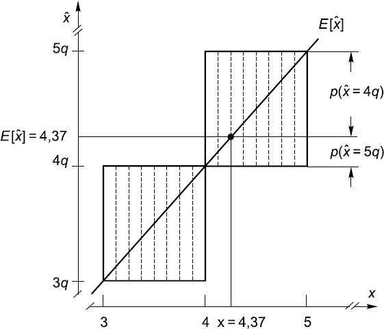
Figure 4.5 Illustration of quantizing performed according to Model 2 in detail.
4.1.3 Rationale of Randomizing
The positive effect due to randomizing the quantization operation is actually obtained as a result of two procedures: randomizing the rounding off of signal instantaneous values and processing the randomly quantized signal. The simplest processing is simply averaging. Naturally, the deterministically quantized signals might be processed in this way as well. It is therefore of some interest to evaluate and compare the effect obtained when averaging is applied to both deterministically and randomly quantized signals.
In addition, it can be said that randomized quantizing is a linear operation if it can be accepted that the output signals are represented in statistical terms, i.e. as estimates of the expected quantized signal values. This obviously requires averaging of the particular quantized signal samples, which may or may not be appropriate from the viewpoint of subsequent signal processing.
Unlike deterministic quantizing, randomized quantizing is sensitive to small increments of signals, which cause proportional increases in output Ê[![]() ]. This kind of quantizing can therefore be used for applications where it is desirable to use rough quantizing. It is of practical interest not only from the viewpoint of reducing the bit streams representing quantized signals. What is more important is the fact that quantizers, when they contain only a few comparators, can be built as extremely broadband devices. Such quantizers, or specialized ADCs, could be very valuable for ultra-high frequency applications. Moreover, this type of relatively simple specialized ADC can be successfully used even for relatively complicated signal processing such as correlation and spectral analysis.
]. This kind of quantizing can therefore be used for applications where it is desirable to use rough quantizing. It is of practical interest not only from the viewpoint of reducing the bit streams representing quantized signals. What is more important is the fact that quantizers, when they contain only a few comparators, can be built as extremely broadband devices. Such quantizers, or specialized ADCs, could be very valuable for ultra-high frequency applications. Moreover, this type of relatively simple specialized ADC can be successfully used even for relatively complicated signal processing such as correlation and spectral analysis.
Rough deterministic and rough randomized quantizing schemes differ noticeably. A single-threshold level deterministic quantizer does not give much information about the input signal. While it is possible to measure the time intervals between signal crossings of the threshold level, none of the signal basic parameters can be estimated. The randomized single-threshold level quantizing process is much more informative. By processing the randomly quantized signals presented in the form of stochastic bit streams it is possible to estimate the mean value of the original signal and to measure its peak or amplitude values.
4.2 Deliberate Introduction of Randomness
Randomness is deliberately introduced into the quantization process to perform the rounding-off operation in a probabilistic way. This means that a signal instantaneous value xk within a range (0, q) is rounded off to the values 0 or q depending on results of comparing it to a randomly generated value ξk uniformly distributed within the same range. If xk< ξk, the value of xk is rounded off to 0 and if xk> ξk then the result of rounding-off is equal to q. Therefore the outcome of the probabilistic signal rounding-off depends not only on the signal value itself but also on the random variable ξ. Even a small signal value with some probability may be rounded off to q and when that happens the particular quantization error is large. Such randomization of quantizing can be beneficial only under certain conditions. It does not make sense to randomize the quantization of separate uncorrelated signal sample values as it would then lead to worse, not better, results. On the other hand, the properties of the signal quantized in this way, as shown below, are attractive. In general, this approach might be advantageous for applications where sampled signals are quantized continuously for some duration of time and the quantized signals are later properly processed. This can be implemented in various ways.
4.2.1 Various Models
If the idea is accepted that it is possible to use time-variant threshold levels for performing signal quantization, various models for randomized quantization might be suggested. They differ first of all in the underlying statistical relationships, according to which sets of random threshold levels are formed. In some other cases the definitions of the quantized signals differ as well. Three models of randomized quantization have been selected from a relatively large quantity considered over a long period of time. They are discussed below and recommended for practical applications. In fact, they are versions of one and the same basic Model 1, illustrated in Figure 4.5.
Model 1
The intervals between the reference threshold levels (Figure 4.3), according to this model, are random and each set of levels used at time instants tk−1, tk, tk+1, tk+2, . . . differs from every other set. The threshold level ordinates qki should therefore be denoted by double indices indicating the time instant (first index) and the respective threshold level ordinate (second index). The threshold level sets are formed in such a way that
![]()
where τki is a realization of the random variable.
Note that Equation (4.3) actually describes the same relationship as the one on which the additive random sampling scheme is based. As with random sampling, the intervals between the randomly positioned threshold levels {qki, qk(i−1)} should also be identically distributed and mutually independent. This is required to ensure that the quantized signal values ![]() k are unbiased, i.e. to ensure that E [
k are unbiased, i.e. to ensure that E [![]() k] = xk. In the case of Model 1,
k] = xk. In the case of Model 1,
![]()
where nk is the number of threshold levels below the corresponding signal value xk and ![]() is the mean value of the intervals between the threshold levels.
is the mean value of the intervals between the threshold levels.
It is apparent from Figure 4.3 that implementation of this quantization scheme is not simple. Since it makes sense to randomize the quantization of mostly highfrequency signals, the threshold level sets needed for that have to be generated during short time intervals {tk+1 – tk}. This is not easy because the required statistics of those levels should satisfy certain requirements. For instance, the reference value in this case is the mean value of the intervals between the threshold levels ![]() . Therefore the stability of this parameter has to be secure. This threshold forming process will not be dealt with in detail because quantization in accordance with Model 1 is not really recommended for analog-to-digital conversions of time-variant signals. This approach is much better suited for quantization of short time intervals, phase angles and other related physical quantities. For these applications, the quantization thresholds are in the form of short pulses generated at proper time instants and the involved techniques are those used for randomized sampling. They are considered in Chapter 6.
. Therefore the stability of this parameter has to be secure. This threshold forming process will not be dealt with in detail because quantization in accordance with Model 1 is not really recommended for analog-to-digital conversions of time-variant signals. This approach is much better suited for quantization of short time intervals, phase angles and other related physical quantities. For these applications, the quantization thresholds are in the form of short pulses generated at proper time instants and the involved techniques are those used for randomized sampling. They are considered in Chapter 6.
The randomized quantization of time intervals can therefore be analysed using virtually the same relationships as those derived in Chapter 6 for randomized sampling. Of course, this is also true for amplitude quantization performed in accordance with Model 1. For instance, it can written that the expected value of the quantized signal is
![]()
The expected number of threshold levels within the interval [−X0, xk] can be determined by applying the function derived in Chapter 3. In this case,
![]()
Substituting Equation (4.6) into expression (4.5) gives
![]()
Therefore the expected value of a quantized signal value is equal to the corresponding signal value. In this sense the quantization is a linear operation. Such quantization is unbiased, which holds even for very crude quantization.
To ensure the correct performance of quantizers built according to the requirements of Model 1, only one parameter of the random threshold level sets, namely the mean value ![]() , should be kept constant at a given level. Other statistical parameters may slowly drift so long as they remain within some relatively broad limits. Instantaneous input-output characteristic is given in Figure 4.6.
, should be kept constant at a given level. Other statistical parameters may slowly drift so long as they remain within some relatively broad limits. Instantaneous input-output characteristic is given in Figure 4.6.
Model 2
This model is more versatile and practical. In fact, this is a version of the generic Model 1, characterized by σ/![]() ⇒ 0, where σ is the standard deviation of the intervals {qki – qk(i−1). Under these conditions, the intervals between thresholds are constant and equal to the quantization step q. Randomized quantization performed in accordance with this model is also illustrated by Figure 4.3. This time diagram is given for quantization of a unipolar signal. The equidistant threshold level sets change their positions randomly at time instants tk−1, tk, tk+l, ....
⇒ 0, where σ is the standard deviation of the intervals {qki – qk(i−1). Under these conditions, the intervals between thresholds are constant and equal to the quantization step q. Randomized quantization performed in accordance with this model is also illustrated by Figure 4.3. This time diagram is given for quantization of a unipolar signal. The equidistant threshold level sets change their positions randomly at time instants tk−1, tk, tk+l, ....

Figure 4.6 Instantaneous input-output characteristic of Model 1.
To ensure that the quantized signal value
![]()
the interval q0k between the zero level and the first threshold above it should be distributed uniformly within the range [0, q]. Note that the random interval q0k at each quantization instant tk determines the positions not only of the first but also of all the other evenly spaced threshold levels of the respective set. This means that only one random variable has to be generated and stabilized, which simplifies the implementation of this quantization method considerably. The quantization results in this case are, of course, unbiased.
Model 3
This model is also a version of Model 1, differing from it only by the definition of the reference value. Instead of relying on a relatively inconvenient basic measure ![]() , this quantization scheme relies on a reference that can be stabilized more accurately: a constant voltage level X representing the upper boundary of the signal range. The quantized signal in this case is given as
, this quantization scheme relies on a reference that can be stabilized more accurately: a constant voltage level X representing the upper boundary of the signal range. The quantized signal in this case is given as
![]()
where mk is the number of threshold levels falling at the time instant tk within the interval [0, X]. It follows from this equation that a quantization scheme such as this does not require the stability of the involved random processes. This is certainly a desirable feature, making this technique well suited for practical applications including short time interval measurements.
Note that the quantized signal values calculated according to Equation (4.5) are in fact biased. To confirm this, the quantized signal ![]() can be considered as a function of the variables n and m. The Taylor expansion of this function around the point (E[n], E[m – n]) is
can be considered as a function of the variables n and m. The Taylor expansion of this function around the point (E[n], E[m – n]) is

where R is the remaining term.

This means that the bias of the quantised signal ![]() is equal to E[R].
is equal to E[R].
Calculations show that in many cases this bias can be ignored because it is relatively small. For instance, when ![]() = 0.5X and
= 0.5X and ![]() = 0.2X the error due to this bias is no more than 3.5% and 0.27% of the maximal statistical error value respectively (99% confidence level). Moreover, this bias error rather nontypically decreases when the quantized signal values are averaged.
= 0.2X the error due to this bias is no more than 3.5% and 0.27% of the maximal statistical error value respectively (99% confidence level). Moreover, this bias error rather nontypically decreases when the quantized signal values are averaged.
It is shown in Chapter 19 that this randomized quantization model is especially well suited for measuring short time intervals with nanosecond or even picosecond resolution. At these applications, the quantizing stream of pulses generated at random time instants in accordance with the given relationships is used as an instrument for comparing the time interval being measured with a reference interval. The point is that the characteristics of the used random pulse sequence may drift around their nominal values without degradation of the measurement precision as long as the reference interval is kept stable.
4.3 Quantization Errors
Whatever quantization principle is applied, the following can always be written:

where∊(t) is quantization noise. An illustration of∊(t) produced by the deterministic quantization of a signal is shown in Figure 4.2(b). When sampled signals are quantized, expression (4.12) is slightly modified. Then

and the quantization noise is represented by the sequence of respective quantisation errors ∊k.
Quantization techniques are usually characterized not only by the time diagrams and input–output relationships described but also by the properties of the corresponding quantization errors or noise. In the case of deterministic quantizing, the errors {∊k} are usually assumed to be uniformly distributed in the range [−0.5q, 0.5q]. It is also assumed that
![]()
It follows from these assumptions that there are no bias errors and that statistical quantization errors have the following variance and standard deviation:

or, in terms of Equation (4.1),

These simple formulae are appropriate for quantizer evaluations in rough calculations and for other simplified calculations. For many multibit quantizer applications a more complicated analysis is often not required.
However, the assumption that the quantization errors are distributed uniformly does not hold in cases where rough quantization is applied or when signal amplitudes are comparable with the quantization step q. The quantization processes then need to be characterized in more detail.
4.3.1 Probability Density Function of Errors
Rough randomized quantization may often substitute multibit deterministic implementation of this operation. In many cases such randomized quantization proves to be more efficient because it allows the required level of precision to be achieved by processing a smaller volume of bits. However, at the same time the application success of this technique depends on the attention paid to details. Consider the vital error characteristics of such a rough randomized quantization performed by using relatively few threshold levels. An essential characteristic is the probability density function of errors defining the distribution of the quantization errors of the quantization models.
Model 1
The probability density function for an input signal x (t) ∊ [0, X] is denoted by ϕ(x). Assume that at the quantization instant the signal is equal to x. Then the probability that there will be n threshold levels inside the interval [0, x]is
![]()
where P(n) is the probability distribution function of the nth threshold level. For any value of the signal, x = n![]() + ∊ can be written. Hence the probability density function of the quantization error is defined as
+ ∊ can be written. Hence the probability density function of the quantization error is defined as

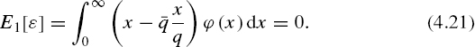
Note that the indices at Ψ1 (∊) and other parameters following indicate the number of the corresponding quantization model considered. The expected value of the quantization error may be given as

To simplify the equation it is worthwhile to introduce and use the following function:

When −X ⇒ ∞, H(x) = x/![]() . In addition,
. In addition,

If these considerations are taken into account,
The variation of the quantization error
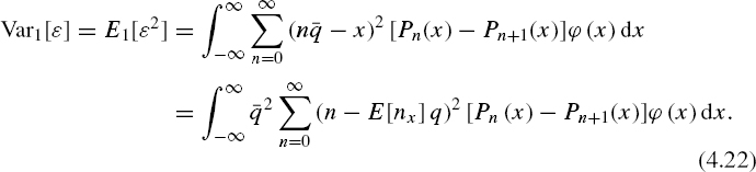
As it can be written that

Equation (4.22) may be given in the following form:

On the basis of function (4.19), the variation Var[nx] is defined as

Model 2
In this case ∊ ∊ [−q,q] and the following equalities hold:

The probability density function Ψ2(∊) of the quantization error can be obtained on the basis of these relationships. By analogy with Equation (4.17), it can be written that

Equation (4.21) can be used to obtain the expected quantization error E2[∊]. Following the previous reasoning, it is easy to show that
![]()
The general expression for Var2[∊] is given by Equation (4.24). Substituting Equation (4.22) into Equation (4.24) yields

A particular average probability density function of a quantized signal is now introduced:
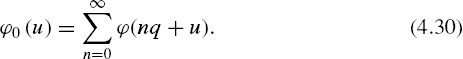
This function is obtained by stacking all the subintervals of ϕ(x) for x ∊ [nq, (n + 1)q] on the interval [0, q] and subsequently summing them. When relatively many threshold levels are used for quantizing, ϕ0 (u) ~ 1/q and it follows from Equation (4.29) that
![]()
The quantization error is characterized by this variance in cases where the probability density function for ∊ ∊ [−q, q] is triangular. Indeed, substituting ϕ0(u) into Equation (4.27) gives

It follows from Equations (4.17) and (4.27) that the probability density functions Ψ1(∊) and Ψ2(∊) in principle depend on the input signal x. When q decreases, i.e. when the number of threshold levels used for quantization increases, this dependence weakens and both of these functions tend to become triangular.
The probability density function Ψ2(∊) is illustrated in Chapter 5, where it is compared with analogous functions characterizing other quantization methods.
4.3.2 Variance of Randomly Quantized Signals
Two of the three quantization models considered here guarantee that the quantized signal values ![]() are unbiased and the quantization bias errors in Model 3 are usually negligible. Hence the dominating quantization errors are random and are characterized by the variance of
are unbiased and the quantization bias errors in Model 3 are usually negligible. Hence the dominating quantization errors are random and are characterized by the variance of ![]() . Of course, these errors depend on the particular quantization conditions described by Models 1, 2 and 3.
. Of course, these errors depend on the particular quantization conditions described by Models 1, 2 and 3.

Figure 4.7 Plots of variances Var[n] versus normalized signals characterizing various quantization schemes
Model 1
When randomized quantization is performed as defined by Model 1, ![]() = n
= n![]() x and
x and
![]()
Var1[n] is defined by Equation (4.25), which shows that this variation depends on the probability density function of the signal x, as well as on the standard deviation of the random intervals{qij – qi(k−1)}. The statistical quantization errors are apparently less significant for smaller values of σ/![]() . The dependence of Var1[n] on x/
. The dependence of Var1[n] on x/![]() is illustrated in Figure 4.7. These diagrams have been calculated on the basis of Equation (4.25). Curves 1 to 4 correspond to the randomized quantization carried out under the condition that the probability density functions of the intervals between the threshold levels are normal. They are given forσ/
is illustrated in Figure 4.7. These diagrams have been calculated on the basis of Equation (4.25). Curves 1 to 4 correspond to the randomized quantization carried out under the condition that the probability density functions of the intervals between the threshold levels are normal. They are given forσ/![]() = 0.3, 0.2, 0.1 and 0.05 respectively. Line 5 corresponds to extremely randomized quantization when the ordinates of the threshold levels at each time instant tk correspond to the Poisson point streams. Thus this line is really a boundary on the left-hand side. All other possible relationships characterizing randomized quantization performed according to Model 1 are to the right or below it. At this extreme quantization mode
= 0.3, 0.2, 0.1 and 0.05 respectively. Line 5 corresponds to extremely randomized quantization when the ordinates of the threshold levels at each time instant tk correspond to the Poisson point streams. Thus this line is really a boundary on the left-hand side. All other possible relationships characterizing randomized quantization performed according to Model 1 are to the right or below it. At this extreme quantization mode
![]()
Quantization, as carried out by this model, is characterized by curve 6. In this case, the variance of ![]() is defined as
is defined as
![]()
For x ∊ [nq, (n + 1)q] the function H(x) = n. In this case, it follows from Equation (4.25) that

Therefore, under these conditions, the variances of the quantized signals are represented by parabolas assuming zero values at points where x = nq.
Model 3
Variance Var3[![]() ], characterizing randomized quantization executed in accordance with Model 3, obviously depends on Var3[m], Var3[n], Var3[m – n]. All of these can be calculated from Equation (4.25). It follows from Equation (4.10) that
], characterizing randomized quantization executed in accordance with Model 3, obviously depends on Var3[m], Var3[n], Var3[m – n]. All of these can be calculated from Equation (4.25). It follows from Equation (4.10) that

As the covariance
![]()
then

4.4 Quantization Noise
Time sequences of quantization errors are known as quantization noise. When the quantization operation is performed on a sampled signal, quantization noise is a discrete-time random process. The properties of this noise determine the usefulness of the corresponding quantization scheme. For a further comparison of the deterministic and randomized quantization approaches this section will consider the respective quantization noises. It is assumed that randomized quantization is carried out according to Model 1. Realizations of the quantization noise characterizing deterministic and randomized quantization are given in Chapter 5. It is clear that the various types of quantization noise will differ considerably.
The noise of deterministic quantization varies within the range [−0.5q, +0.5q] and during some time intervals the envelopes of this noise repeat respective segments of the signal x(t). The polarity of the errors is determined only by the input signal values. The range of randomized quantization noise is twice as large, i.e. [−q, +q]. The envelopes of this noise also repeat the corresponding parts of the signal, although particular errors can assume either positive or negative values at random, i.e. the value of the error is either equal to ∊(+) or to ∊(−). At each quantization instant ∊(+)k + ∊(−)kk = q. The appearance of the larger error is less probable. It can be written that

where Pr[∊k = ∊(+)k] and Pr[∊k = ∊(−)k] are the probabilities of the error ∊k assuming positive or negative values respectively. Of course,
![]()
This uncertainty in error polarity, typical of randomized quantization, is beneficial because it decorrelates the input signal and its corresponding quantization noise.
4.4.1 Covariance between the Signal and Quantization Noise
Since the envelopes of quantization noise follow the corresponding parts of the input signal waveform, it seems that quantization noise is statistically dependent on the signal. To assess the degree of dependence between these two processes, consider a randomized quantization performed in accordance with the quantization Model 2. Statistical relationships of this kind are more pronounced in coarse quantization. Therefore, without loss of generality, one threshold randomized quantization scheme can be considered with x(t) ∊ [0, q].
If at the quantization instant tk the input signal is xk, the quantized signal ![]() k can be either 0 or q. Hence the quantization error ∊k =
k can be either 0 or q. Hence the quantization error ∊k = ![]() k – xk is either equal to −xk or to (q – xk). The probabilities of the respective events are
k – xk is either equal to −xk or to (q – xk). The probabilities of the respective events are

It can be written that the covariance between ∊k and xk is

This result is unexpected. Indeed, as can be seen from Equations (4.26), there is a strong dependence of ∊k on xk. It is therefore hard to accept that the corresponding covariance is equal to zero. Nevertheless, the covariance between ∊k and xk is equal to zero.
4.4.2 Spectrum
The extremely coarse quantization scheme is also convenient for determining the spectral characteristics of randomized quantization. Assuming that quantizing is performed according to Model 2 and taking into account Equation (4.39), the autocovariance function of quantization noise for all m ≠ 0(m = 0, 1, 2,...) is given as

where p(xk, xk+m) is the two-dimensional probability density function. It follows from this equation that

where σ2∊ is the variance of the quantization noise. This result also holds for multithreshold randomized quantization. Of course, the appropriate variance characterizing the particular quantization noise should be substituted into Equation (4.42).
It follows from Equation (4.42) that the spectral density function of quantization noise {∊ (kΔt)} is given as

Note that the covariance between the signal and quantization noise, as well as the autocovariance function of this noise, is obtained under the assumption that the signal is sampled periodically. Under this condition and taking into account the sampling theorem,

As quantization Models 1 and 2 show, quantizing according to Model 1 is randomized to a greater degree than quantizing as defined by Model 2. The randomization level for Model 1 is characterized by the ratio σ/![]() . When the value of this ratio decreases, the correlation between quantizing errors increases. However, even at σ/
. When the value of this ratio decreases, the correlation between quantizing errors increases. However, even at σ/![]() = 0, the quantization noise is white; hence it is also white for σ/
= 0, the quantization noise is white; hence it is also white for σ/![]() > 0 and Equation (4.44) is also true for quantizing performed according to Model 1.
> 0 and Equation (4.44) is also true for quantizing performed according to Model 1.
Bibliography
Bennet, W.R. (1948) Spectra of quantized signals. Bell Syst. Tech. J., 27(7), 446–72.
Bilinskis, I. (1976) Stochastic signal quantization error spectrum (in Russian). Autom. Control Comput. Sci., 3, 55–60.
Bilinskis, I. and Mikelsons, A. (1992) Randomized Signal Processing. Prentice-Hall International (UK) Ltd.
Brannon, B. (1996) Wide-dynamic-range A/D converters pave the way for wideband digital-radio receivers. In EDN, 7 November 1996, pp. 187–205.
Brannon, B. Overcoming converter nonlinearities with dither. Analog Devices, AN-410, Application Note.
Brodsky, P.I., Verjushsky, V.V., Klyushnikov, S.N. and Lutchenko, A.E. (1970) Statistical quantization technique using auxiliary random signals (in Russian). Voprosy Radioelektroniki Ser. obshchetekhnic, 3, 46–53.
Corcoran, J.J., Poulton, K. and Knudsen, K.L. (1988) A one-gigasample-per-second analog-to-ditial converter. Hewlett-Packard J., June, 59–66.
Demas, G.D., Barkana, A. and Cook, G. (1973) Experimental verification on the improvement of resolution when applying perturbation theory to a quantizer. IEEE Trans. Industr. Electron. Control Instr., IECI20(4), 236–9.
Gedance, A.R. (1972) Estimation of the mean of a quantized signal. Proc. IEEE, 60(8), 1007–8. Jayant, N. and Rabiner, L. (1972) The application of dither to the quantization of speech signals. Bell Syst. Tech. J., 51(6), 1293–304.
Rabiner, L. and Johnson, J. (1972) Perceptual evaluation of the effects of dither on low bit rate PCM systems. Bell Syst. Tech. J., 51(7), 1487–94.
Veselova, G.P. (1975) On amplitude quantization with overlapping of interpolating signals (in Russian). Avtomatika i Telemekhanika, 5, 52–9.