19

Estimation of Object Parameters

To achieve the best results, algorithms for processing digital signals should take into account the specific features of the digital signals to be processed. These features to a large extent depend on the chosen and used sampling and quantizing methods. The latter, in turn, depend on the given task to be solved. Thus the task actually dictates the requirements that have to be satisfied when choosing and using signal digitizing and processing techniques.

In the previous chapters an attempt has been made to show that signals could be digitized and processed in various ways and that it is essential to use appropriate methods and techniques. This helps to meet requirements of many different applications and the discussed methods for signal digitizing and processing actually cover a wide application field where good results can be achieved. On the other hand, in some areas it is easier to be successful than in others. One such application area where it is relatively easy to get good results at solving challenging tasks is considered in this chapter. This is the area where signal processing is carried out to identify objects and to evaluate their parameters by analysing the signals reflecting the reaction of these objects to some excitation signals. The parameters and characteristics of the excitation signals are usually known. Access to this valuable information makes it easier to keep algorithms relatively simple and to achieve high performance.

19.1 Measuring the Frequency Response of Objects

Identification of objects by observing and analysis of their reaction to specific test signals is a task often met. Many kinds of signal processing systems fulfil tasks in this category. The existing systems of this type in many cases are good enough. Nevertheless, with the advancement of high technologies, the requirements are growing in this area. The nontraditional signal processing techniques discussed in this book might prove to be beneficial for achieving significant widening of the frequency range where these systems could operate, simplification of the system designs and/or increasing their operational speed. Simplified block diagrams of basic and suggested typical systems of this kind are given in Figure 19.1.

Figure 19.1 Block diagrams of systems for measuring the frequency response of objects. (a) prototype; (b) improved version

The basic structure of the most popular system for measuring the frequency response, often considered as a network analyser and shown in Figure 19.1(a), is well known. Typically, it contains a variable frequency single tone generator and two vector voltmeters connected to the input and output of the electronic device to be tested by measuring its frequency response and other derivative parameters. The frequency response is measured by changing the frequency of the generated input signal step by step over the whole frequency range of interest. At each frequency setting, amplitudes and phase angles of the signals at the input and output of the device under test are measured and the data obtained in this way are used to calculate all needed parameters.

An improved version of this type of system is given in Figure 19.1(b). The structure and performance of it differs in the following ways:

1. A multifrequency signal source is used to speed up the whole measurement process by avoiding a repetition of the measurement process step by step for each separate frequency.
2. A spectrum analyser rather than a vector voltmeter is used for high-speed estimation of the frequency response of the electronic device being tested by processing a single shot of the output signal.
3. The multifrequency signal source generates the test signal using specified parameters, including the phase angles for all frequency components, leading to the possibility of using a single rather than two spectrum analysers and thus reducing the complexity and production costs of the system.
4. Pseudo-randomized sampling techniques are used to achieve and provide for a high-resolution vector spectrum analysis of wideband signals in the frequency range up to a few GHz.

While all the elements of the system determine its performance, the multifrequency test signal generator plays a special role. In an ideal case, the generated excitation signal contains discrete frequencies covering the required density for the whole frequency range within which the object behaviour is to be observed. It is not easy to cover all of it at one go if this frequency range is indeed wide. It is more realistic to generate multifrequency test signals covering some part of the whole frequency range of interest. Then the test measurement procedure has to be repeated several times. Obviously, much depends on the frequency band that could be covered by a single realization of the test signal.

There is some risk when just one channel spectrum analysis is used. Then most of the responsibility for phase-locking of the generated frequency components of the excitation signal in the predetermined positions is put on the excitation signal synthesizer. There may also be some hidden problems as various impedances may impact on the measurement accuracy. It is necessary to check whether this effect can be kept under control and whether one spectrum analyser measurement scheme can be applied in all cases.

All these considerations show that the performance of the whole test system depends to a large degree on the capabilities of the multifrequency test signal synthesizer. An approach to such signal synthesis, based on exploitation of the alias-free signal sampling techniques, is discussed in the next section.

19.2 Test Signal Synthesis from a Sparsely Periodically Sampled Basis Function

The task of analog signal synthesis from discrete data comes up frequently and the ways used to resolve it by using a DAC are well known. However, that is true only if and when the classical requirements are met, specifically when the corresponding discrete data block to be transformed into an analog signal is actually represented by a sample value sequence taken from a certain basis function under conditions where at least two sample values are taken in the time interval equal to the period of the highest frequency present in this function. Then no aliasing takes place and there are no problems. Therefore this is the preferred way to perform analog signal synthesis whenever the mentioned conditions can be satisfied. However, the operational speed of DACs is limited and, consequently, the highest frequency of the signal to be synthesized in this way cannot exceed a certain boundary determined by the switching speed of the sufficiently high bit rate DAC available. The accumulated experience of successful suppression of various negative effects due to aliasing suggests that it is worth looking for a way to avoid this synthesis limitation.

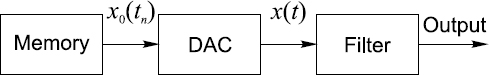
Figure 19.2 Generalized structure for continuous signal x(t) synthesis from digital data

The generalized model of the continuous signal x(t) synthesis from digital data is given in Figure 19.2. To obtain a continuous or analog signal x(t), a related basis function x₀(t) is formed. Typically that is done by a computer, forming it as a sum of a finite number of sinusoidal components. As parameters (frequencies, amplitudes and phase angles) depend in some way on the analog signal to be synthesized, their values, as well as the sampling frequency f_s, should be calculated on the basis of the algorithm used for synthesis. The approach to such analog signal synthesis will be discussed further. At this stage it should simply be noted that these signal component parameters are fixed and, consequently, sample values x₀(t_n), n = 1, 2,..., N, of the basis function can be calculated and stored in a memory. These digital values are than passed at the sampling rate f_s to a DAC performing their conversion into a kind of analog signal, which changes its values in an idealized stepwise way, as shown in Figure 19.3. The synthesized signal is taken off the output of the filter.

It can be seen from the diagrams in Figure 19.3 that the values of the basis function change continuously while the DAC output signal remains at some level for relatively long time intervals, which are longer than the period of the basis function. The DAC output signal certainly does not look similar to the given basis function. The question arises as to what kind of properties this staircase signal prossesses and whether it is possible to obtain such a signal with the required properties.

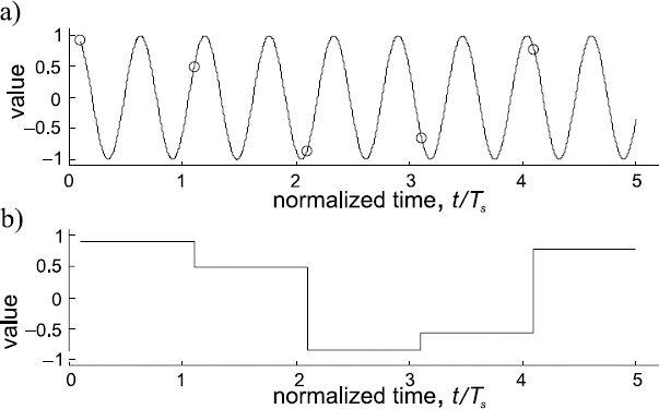
Figure 19.3 Illustration of analog signal synthesis in the case of periodic sampling; (a) basis function x₀(t) with its sample values x₀(t_n) indicated; (b) signal at the output of the DAC

The spectrum of the DAC output signal is obviously unlimited, even in the case of the low-frequency basis function x₀(t). On the other hand, this spectrum clearly depends both on the basis function and the sampling frequency f_s. This relationship determines the properties of the synthesized signal and analysis of it should provide the answer to the question of how feasible it is to achieve the possibility of developing a high-performance signal synthesizer. To find the answer to the question of how feasible it is to synthesize analog signals under conditions where the requirements of the sampling theorem are not met, it is necessary to establish how feasible it is to transfer the frequencies of the basis function to the DAC output signal, even when those frequencies exceed the sampling rate, and whether it is possible to synthesize a signal having the required frequencies not corrupted by aliases.

In order to get answers to these and other similar questions, there will be a focus on the estimation of the spectra of the stepwise DAC output signal that clearly depends on the sampled basis function and on sampling conditions.

19.2.1 Synthesis in the Case of Monoharmonic Basis

Assume that the basis function x₀(t) is monoharmonic:

It follows from the explained synthesis approach that the DAC output signal is given as

As sampling is periodic, t_n = nμ, where μ = 1/f_s is the sampling time interval. The spectrum of the signal x(t) in this case can be defined in the following way:

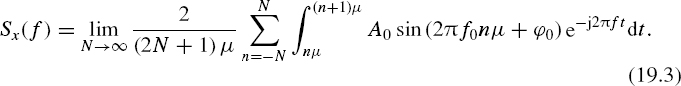
Consider the real a_x(f) and the imaginary b_x(f) parts of this Fourier transform separately. Then

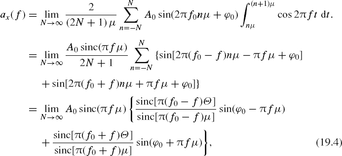
where Θ = (2N + 1) μ and sinc(x) = sin x/x. The coefficient b_x(f) is obtained in a similar way:

The transition N → ∞ is performed in Equations (19.4) and (19.5). Then

where r = 0, 1, 2, 3,... .

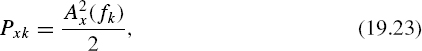
The Fourier transform module A_x(f), actually representing the amplitude of the signal x(t) at the frequency f, is derived from Equations (19.6) and (19.7) as

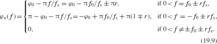
It follows from Equation (19.8) that the signal x(t) has discrete components: it contains the component at frequency f₀ and all aliasing frequencies corresponding to it and to the sampling frequency f_s. Equation (19.8) defines the amplitudes of these components. They decline in accordance with |sinc(π f μ)|. The component at the lowest frequency from the frequency row 0 < f = ± f₀ ± rf_s, rather than the component at the frequency f₀, has the maximal value amplitude. However, it should be noted that, in the case of periodic sampling, any frequency from the row 0 < f = ± f₀ ± rf_s, r = 0, 1, 2,..., is represented by one and the same data set at the time instants t_n, n = 1, 2,... . It follows from Equations (19.6) and (19.7) that the phase spectrum of the DAC output signal is given as

19.2.2 Synthesis in the Case of Multifrequency Basis

Consider the case where the basis function x₀(t) is actually a sum of a certain number of sinusoidal components:

As the Fourier transform is a linear operation, the Fourier coefficients a_x(f) and b_x(f) for the DAC output signal x(t) will differ from zero only at frequencies f_k, k = 1, 2,..., and at all corresponding aliasing frequencies:

Therefore the described synthesis transforms every sinusoidal component of the basis function into an infinite sum of sinusoidal components at frequencies defined by (19.11) and with amplitudes and phase angles determined by Equation (19.8) and (19.9) if f₀, A₀ and ϕ₀ are substituted by f_k, A_k and ϕ_k respectively. The component at the zero frequency or at frequencies equal to an integer number of f_s, i.e. if f_k = rf_s, r = 0, 1, 2,..., represents an exception. In this case, all discrete values of that component are the same and it is accepted that this is a constant level and, consequently, the DAC output signal is also constant. Therefore if the basis function contains a component at any of the frequencies f_k = rf_s, r = 0, 1, 2,..., it transforms into a constant level equal to A_k sin ϕ_k.

All of the basis function frequencies clearly have to be chosen so that they do not overlap the frequencies of the rest of the basis function components or their aliases. Therefore any frequency of a basis function component f_m, m = 0, 1, 2,..., K, has to meet the following condition:

where φ is an empty multitude while f_kr is determined by (19.11). The amplitude spectrum of the DAC output signal, for the case where the basis function is given by

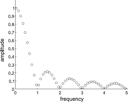
Figure 19.4 Amplitude spectrum of the DAC output signal in the case of a multifrequency basis function

is shown in Figure 19.4. The spectrum corresponds to the normalized frequency f_s = 1.

It can be seen from this analysis that when the frequencies of the basis function components cover the Nyquist range uniformly, the components of the DAC output signal cover uniformly the whole frequency axis. However, their amplitudes decline rather rapidly. If the basis function is represented by a sum of sinusoidal components, the DAC output signal has a discrete spectrum. Each of the basis function components at the frequency f_k, if f_k ≠ rf_s, r = 0, 1, 2,..., is transformed into a sum of an infinite number of sinusoidal components with precisely predetermined frequencies, amplitudes and phase angles. Even when the basis function is relatively simple, the obtained synthesized signal can have a rich spectrum with precisely predetermined parameters of all components.

19.3 Test Signal Synthesis from a Nonuniformly Sampled Basis Function

Consider the case where a monoharmonic basis function x₀(t) is sampled nonuniformly. The idealized DAC output signal x(t) formed in this case is shown in Figure 19.5.

Figure 19.5 Illustration of forming the DAC output signal in the case of nonuniform sampling of the basis function

The basis function x₀(t) with its sampled values marked at time instants t_k are shown in Figure 19.5 by a continuous line while the signal x(t) at the DAC output is given by a dashed line. The aim is to find what are the properties of the analog signal obtained in this case and how they differ from the properties of a similar signal formed in the case of sparse periodic sampling.

19.3.1 Spectrum of the Synthesized Signal

The spectrum of the analog signal x(t) at the DAC output in this case is defined as follows:

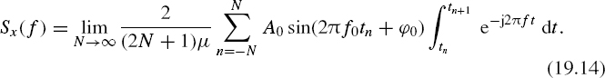
The notation μ_n = t_n+1 – t_n is introduced. The Fourier coefficient can be defined as

Suppose that the sampling intervals are formed as follows:

where the mean value of these intervals is μ = Mδ, M is a positive integer, δ is the digit for the intervals m_n, r_n = 0, ±1, ±2,..., ±m, and f₀ < ¹δ. Therefore ₂ there are (2m + 1) various intervals m_n. It is assumed that all of them are repeated for an equal number of times. The time instant t_n is defined as

This kind of sampling point process is statistically equivalent to a periodic point stream with random skips obtained in the case where the sampling frequency is equal to 1/δ. From Equation (19.15), by taking into account (19.16), it is found that

By taking into account the properties of the considered sampling point process, the following sum can be calculated:

Substitution of Equation (19.18) into Equations (19.17) yields

The second Fourier coefficient b_x(f) is obtained in a similar way:

Equations (19.19) and (19.20) lead to the module of the Fourier transform:

It can be seen from Equations (19.21) that the analog signal has a discrete component at frequency f₀ of the basis function and also has all aliasing frequencies corresponding to frequencies f₀ and 1/δ. Now it should be checked whether there are only discrete components present in the synthesized analog signal x(t) or whether there are also additional noisy components with a continuous spectrum. The frequencies of the discrete components in increasing order are the following:

Their power, on the basis of Equations (19.21), can be calculated as

where f_k is the kth frequency of the sequence (19.22).

If the pseudo-random sampling process is properly arranged, the power of the aliasing components is usually negligible. Therefore, almost all of the total power of all signal x(t) discrete components is concentrated within the first component at frequency f₀. However, the signal x(t) contains a component with a continuous spectrum, in other words, noise.

19.3.2 Multifrequency Signal Synthesis

The properties will be established of the DAC output signal in the case of a nonuniformly sampled basis function represented by a sum of a certain number of sinusoidal components, when the basis function is described by Equation (19.13) at K > 1. It has been already shown that when the basis function is sampled nonuniformly with the smallest time digit δ, any sinusoidal component of it transforms into a sum of an infinite number of sinusoidal components with given frequencies, amplitudes and phases, plus noise due to the cross-interference caused by sampling irregularities. If the value of the time digit is small enough, the aliases relative to the frequency 1/δ could be neglected as their amplitudes are very small. Therefore, in all practically significant cases, it could be assumed that any component of the basis function is transformed into a sinusoidal component at the same frequency and noise. The amplitude and phase angle of this discrete component in the DAC output signal is determined by Equations (19.19) and (19.20) if f₀, A₀ and ϕ₀ are replaced by f_k, A_k and ϕ_k, respectively. The noise has declining spectral density and its power is equal to (A²_k – A²_xk)/2, where A_xk is the amplitude of the DAC output signal discrete component.

Thus, when the basis function x₀(t) is a sum of several sinusoidal components, the obtained analog signal at the DAC output, due to the linearity of the Fourier transforms, will have components at all those frequencies with precisely predetermined amplitudes and phases (defined by Equations (19.19) and (19.20)) in a mixture with the cross-interference induced noise. The amplitude spectrum of the DAC output signal, corresponding to the nonuniformly sampled multifrequency basis function, is given in Figure 19.6(a) for the same basis function (19.13) used before as an example at the discussion of the periodic sampling case. The amplitude spectrum of the analog signal at the output of the DAC, shown in Figure 19.6(b), corresponds to the case of nonuniform sampling of the following basis:

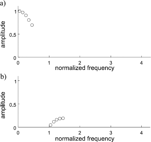
Figure 19.6 Amplitude spectra of the DAC output signal in the case of nonuniformly sampled multifrequency basis function: (a) in the case of basis function (19.13); (b) in the case of basis function (19.24)

As the same frequencies in Equations (19.13) and (19.24) (at the same k) are overlapping, these functions when sampled periodically are equivalent; therefore the corresponding analog signals at the DAC output including their amplitude and phase spectra are also equivalent.

That is not the case when the basis functions are sampled nonuniformly. Then the obtained analog signal contains only those frequencies that are in the spectrum of the corresponding basis function. The amplitudes of the analog signal components are lower for higher frequencies and, with frequencies growing, the power of the additional noise, due to the cross-interference, increases.

19.3.3 Amplitude Equalization

As shown in the previous section, it is possible to synthesize an analog signal from scarce data obtained under conditions when the well-known requirements of the sampling theorem are not met and when the frequencies of the signal to be synthesized exceed half of the DAC switching rate. However, there are also some problems and limitations. First of all, the amplitude of the synthesized sinusoidal signal mainly depends on its frequency. That might cause problems when the analog signal to be synthesized contains a number of frequencies. As that is exactly what is typically needed for the generation of multifrequency test signals, the feasibility of synthesizing such a multifrequency signal will be considered.

Apparently various types of multifrequency test signal are needed. In the context of the considered application, a group of frequencies typically has to be generated around a certain central frequency. Even in this case, there are a number of possible variations. Amplitude spectra of some of them are given in Figure 19.7.

Probably the most popular structure of a multifrequency test signal is the one shown in Figure 19.7(a). All frequencies of it are equidistanced on the frequency axis and amplitudes of all components are equal. However, as discussed further, the price of achieving the equality of amplitudes may sometimes be too high. Quite often it might be better to accept some amplitude variation. Such amplitude variations, if predetermined, should not represent a problem, especially if all component amplitudes are given with sufficiently high precision. This kind of multifrequency signal is given in Figure 19.7(b). The third type of multifrequency signals, illustrated in Figure 19.7(c), differs from the others by the location of the frequencies. In this case the signal components are placed on the frequency axis irregularly at arbitrary places. How beneficial this possibility could be is another question; here the fact is simply demonstrated that the suggested synthesis method would permit that possibility. When the traditional methods for generating such multifrequency test signals are used, it certainly is not simple to provide for this functional feature.

While there are no problems at synthesizing signals with specified frequencies, except that they cannot be placed too closely together, it is quite another situation with the synthesis of multifrequency signals with equal or specified amplitudes of their components. Direct application of the suggested synthesis approach leads to the synthesis of signals with component amplitudes defined by Equation (19.8) and illustrated by Figure 19.4. It follows from Equation (19.8) that when the frequency of a component grows its amplitude declines according to |sinc(π f/f_s)|, where f_s is the sampling frequency. In addition, the amplitudes of components close to frequencies f_s, 2 f_s, f_s,... are very small (frequencies f_s, 2 f_s,... cannot be used as they are transformed into a constant level). Therefore there may be considerable measurement problems at those frequencies where the components are small.

Figure 19.7 Amplitude spectra of various types of multifrequency signals to be synthesized

This problem of how ‘small amplitudes’ might be resolved are considered. There may be at least two distinctly different situations.

19.4 Synthesis of Narrowband and Wideband Signals

Suppose a passband signal z(t) has to be synthesized so that it has a passband in the frequency range (f_min, f_max) and that it is possible to chose a realizable sampling frequency f_s to sample the basis function so that the frequency band (f_min, f_max) can be completely inserted within the interval (if_s, (i + 0.5) f_s), or within the interval ((i + 0.5) f_s, (i + 1) f_s)), where i is a positive integer. To obtain such a signal, the basis function is formed as explained above so that the components of it (f₁, f₂,..., f_K) cover the frequency band (f_min, f_max) with the frequency step δf. This basis function is sampled and a DAC is used to convert the obtained digital signal into an analog signal. Then the DAC output signal is passed through an analog bandpass filter having the same passband (f_min, f_max). The structure of such a synthesizer is illustrated by Figure 19.8.

Figure 19.8 An optional structure for synthesis of a passband signal

In the case of an ideal filter, the amplitudes of the signal z(t) components are determined by Equation (19.8). Therefore if the amplitudes of the basis function components are taken as

where k = 1, 2,..., K, the components of the synthesized signal z(t) will have equal amplitudes A₀. The dynamic range of the signal z(t) is naturally narrower than that of the DAC output signal (t). It is essential to know their ratio. Let D_x and D_z be the dynamic ranges of signals x(t) and z(t). Then their ratio ρ_xz = D_x/D_z.

Figure 19.9 illustrates this approach to signal synthesis where the amplitudes of the basis function have been calculated on the basis of Equation (19.25). Therefore they differ for all components, which leads to equalization of the synthesized signal z(t) component amplitudes, as shown in Figure 19.9(a). The dynamic ranges of signals x(t) and z(t) are obviously different in comparison with the respective dynamic ranges when the output signal component amplitudes are not equalized. In this case ρ_xz = 4.4.

This effect of ρ_xz enlargement rapidly increases if the frequency range (f_min, f_max) approaches any of the frequency points if_s. For instance, if (f_min, f_max) is defined as (1.01 f_s, 1.41 f_s) and again nine components are placed within it with a frequency step of 0.05 f_s then the named ratios ρ_xz for the cases without and with output signal component amplitude equalization are 6.0 and 27.0 respectively. This is due to the fact that the frequency f_min has approached frequency f_s. This can also be seen from Equation (19.25) as near to if_s the function |sinc(π f_k/ f_s)| approaches zero and therefore the corresponding amplitudes of the basis function components have to be large.

Figure 19.9 Synthesis of a narrowband multifrequency signal with component amplitude equalization: (a) amplitude spectrum of the equalized synthesized signal z(t); (b) basis function f₀(t) (dashed line) and DAC output signal x(t) (continuous stepwise line); (c) the obtained signal z(t) at the filter output

Figure 19.10 shows how the amplification coefficient of the basis signal components depends on the normalized frequency (f_k/f_s). The curve is given in the logarithmic scale.

Suppose that the signal z(t) to be synthesized is wideband, the available DAC satisfies the condition f_max – f_min > f_s/2 and the amplitudes of the signal components have to be equalized. In this case it makes sense to subdivide the whole band (f_min, f_max) into sub-bands. After that proper sampling frequency has to be chosen for each one of them so that every frequency subinterval is completely placed within one of the following intervals: (if_s, (i + 0.5) f_s) or ((i + 0.5) f_s, (i + 1) f_s). Therefore this approach to the multifrequency signal synthesis is based on sequential in the time synthesis of a number of signals containing components at frequencies from the corresponding frequency interval.

Figure 19.10 Amplification coefficient of the basis signal components versus the normalized frequency (f_k/f_s)

19.5 Measuring Small Delays and Switching Times

As shown in Chapter 6, the density of sampling points at additive randomized sampling tends to a constant level inversely proportional to the mean sampling interval . When a signal is sampled according to such a sampling model all of its instantaneous values are sampled with equal and constant probability. This valuable feature of the additive sampling model could be beneficially exploited to achieve a high resolution when measuring various signal parameters, such as delays in the reaction of objects to some excitation signals, switching times and differences in signal phase angles. Tasks of this type are apparently based on time-interval measurements.

According to the traditional and most often used approach to digital timeinterval measurements, short clock pulses are generated at a high and stabilized frequency and are then passed through a gate that is opened for the duration of the time interval to be measured. The pulses that pass through are registered by a counter. All is well as long as the clock period is much smaller than the time interval being measured because the ±1 count quantization error, characterizing this measurement method, is acceptable only as long as the number of pulses counted is sufficiently large. Measuring shorter time intervals is more difficult. A fairly efficient solution to this problem is based on the use of randomized pulse sequences mathematically described identically to the description of the additive sampling point processes. Although the randomization techniques concern timeinterval quantizing rather than sampling, the statistical relationships describing both of those procedures are in fact the same.

Block diagrams of two implementation schemes of the suggested randomized time measurement method are given in Figure 19.11. Short pulses generated by random pulse generators represent the quantizing thresholds in this case. These pulse sequences are generated in exactly the same way as in the case of the additive random sampling, i.e. these pulses are formed at time instants given by Equation (6.4). The performance of the schemes shown in Figure 19.11 depends first of all on the perfection of the voltage comparators used to generate the inputs. The comparators should be sensitive wideband devices, capable of detecting small input and reference voltage U₀ differences. Their aperture time should be in the picosecond range.

The time intervals to be quantized are given as durations of the input pulses to be measured at some level determined by the reference voltage U₀. The number of time intervals to be averaged is preset and counter 1 in both schemes is used for counting these intervals in order to stop the quantizing and averaging process after a given number of pulses have been processed. Note that in the case of the scheme in Figure 19.11(b), the number of these time intervals is determined indirectly by actually counting the pulses that fall within time intervals of a constant and known duration, generated by the single-shot time base generator triggered by the appearance of each time interval to be measured. The quantization and averaging results obtained are registered in both schemes by counters 2. The time intervals at the input can be repeated either randomly or periodically.

When the first of these two schemes (Figure 19.11(a)) is used, the result of quantizing a single time interval is given as

where is the mean value of the time intervals between the quantizing pulses. The estimate t of the unknown duration Δt of the time intervals is obtained by averaging N particular results t_i as follows:

Figure 19.11 Block diagrams of two systems for measuring short time intervals

If the pauses between the time intervals to be quantized are large enough, the subsequent particular quantization results can be considered to be statistically independent. Then it can be written that

where Var[n_i] is the variation of the number of quantizing pulses falling within the time interval being measured. In the case of uncorrelated t_i, the random error can be written as

Although this time-interval estimation scheme is simple and practical, the mean value of the time intervals between the quantizing pulses or, in other words, the mean repetition rate of these pulses, should be stabilized, which is certainly a disadvantage.

The second time-interval estimation scheme, shown in Figure 19.11(b), does not have this disadvantage. This improvement is achieved by organizing the estimation process in such a way that the unknown input time intervals are compared with some constant time intervals T, rather than with the parameter ¯ of the pulse sequence used for quantizing. Therefore, in this case, it is the time reference pulse duration T that has to be stabilized. These time reference pulses are generated whenever a time interval to be quantized appears at the input. The reference and input time intervals are quantized in parallel by means of the same quantizing pulse sequence. The quantization results m_i and n_i are entered into the respective counters 1 and 2. It can be written that

Therefore

and the estimate t of the time interval Δt, obtained by averaging N quantization results, is given as

An estimation of Δt can be carried out until either N or the sum of m_i reaches some preset value m. The second approach is preferable and, if it is applied,

In order to carry out the averaged quantizing of time intervals according to Equation (19.31), the capacity of counter 1 should be set equal to m and quantizing should be stopped when this counter is filled up. Then the readout from counter 2 will represent t in time units.

Table 19.1

The advantage of this method for averaged measuring of time intervals, unlike the classical deterministic measurement method, is that it can be applied for evaluating time intervals shorter than when no more than one pulse can fall within the time interval to be quantized and n_i and m_i can assume only the values of 0 or 1. When a quantizing pulse coincides with the time reference interval, the probability that it will also fall within the interval t is equal to t/T. It can therefore be written that

Hence the random estimation error

where t_β is half of the confidence interval corresponding to the confidence probability β.

Note that under the described measurement conditions the random estimation error does not depend on the probabilistic characteristics of the quantizing pulse sequence used. This random quantizing pulse sequence is used in this case as a tool for comparing Δt with the reference value T.

The capabilities of this digital time-interval measurement approach are to some extent illustrated by the experimental measurement results given in Table 19.1. They are obtained under the following conditions: Δt varies in the range 2–10 ns and m = 2⁶ × 10³ calculations were made for the 99% confidence level. The measurements of each Δt value were repeated 20 times.

The described digital short time-interval measurement techniques can be used for various applications based on the delay, phase angle or pulse rise and fall time measurements. This approach has been proved to be of practical value whenever it is essential that the designs of systems are extremely simple. The fact that the time intervals to be measured in this way may be repeated either randomly or periodically at relatively high frequencies might be considered as an additional advantage. It is also relatively easy to achieve high precision. Substantial practical experience has been gained in this field. A number of test and measurement systems used to measure dynamic parameters of various microelectronic elements in the process of their manufacture have been developed on this basis and successfully used. This experience confirms the reality of achieving, in a simple way, subnanosecond resolution usually needed for digital measurements of short time intervals.

19.6 Bioimpedance Signal Demodulation in Real-time

It has been discovered that various processes going on in a human body change the bioimpedance of it and that these changes carry valuable diagnostic information. To obtain this information, a test signal in the form of a constant voltage specific frequency is applied to the body being examined and the bioimpedance signal, reflecting the reaction of the biological object to this excitation signal, is extracted and analysed. To do this, the picked-up signal needs to be demodulated. Realtime demodulation of bioimpedance signals is considered here as an example showing what could be gained by exploiting the digital alias-free signal processing technology.

19.6.1 Typical Conditions for Bioimpedance Signal Forming

Variations of the impedance of a human body due to cardiac activities and breathing lead to modulation of the test signal. Amplitude as well as phase modulation of the carrier takes place. Therefore the modulated carrier has to be processed in a way that leads to the discovery of both the amplitude and phase changes. Demodulation of bioimpedance signals can be performed in various ways. A particular universal solution of this demodulation task could be based on the estimation of both Fourier coefficients at the carrier frequency or at all involved carrier frequencies when a number of test signals at differing frequencies are generated and used. The Fourier transforms in this case need to be performed in real-time.

More often than not, the structure of bioimpedance analysers is multichannel. In addition, bioimpedance signals sometimes have to be obtained at a number of test frequencies simultaneously. This means that a large amount of data typically needs to be acquired and handled. This represents a problem, especially when the bioimpedance signals have to be observed for a long time. Then it is desirable to preprocess the data in a cost-effective way and to compress them before these data are transferred to the host computer. The technical characteristics of this signal preprocessing unit in terms of complexity, volume, power consumption and operational speed depend on the method used for bioimpedance signal demodulation and its hardware and software implementation. Therefore it is essential to develop and use a good enough method for bioimpedance signal demodulation.

It has been found that impedance signals at various frequencies carry different information. This means that the test signal frequencies could vary in a wide frequency range, from relatively low frequencies of about 100 kHz up to 1 GHz. This is one of the conditions that makes this application area well suited for the specifics of the digital alias-free signal processing technology.

The next essential condition that complicates the bioimpedance signal on-line demodulation task considerably is the relatively large number of input signals that need to be processed in parallel. Typically there are 12 inputs, but sometimes even more inputs are needed.

The demodulation task is simplified to some extent by the fact that the modulations are typically within a range of frequencies that is much lower than the carrier frequencies. The cardiac related and breathing processes that basically modulate the test signal are typically in the frequency range not exceeding 1 kHz. Therefore relatively few readings of the Fourier coefficients need to be obtained in a second to present the demodulated signal sufficiently well. That helps to process a number of bioimpedance signals in parallel.

19.6.2 Complexity Reduction of Bioimpedance Signal Demodulation

Analysis of the mentioned considerations has led to the conclusion that the method developed earlier and discussed in Chapter 16 for the complexity-reduced DFT represents a promising option for demodulation of the bioimpedance signals under the given conditions. Using this approach for development of such a system has provided results close to those expected.

The outline of the suggested approach is as follows. In general, the Fourier analysis is accomplished in two stages. In the first stage, the signal to be analysed is formally decomposed on the basis of some rectangular functions assuming only the values −1, 0 and + 1, so this decomposition can be carried out without performing the multiplication operations. In the second stage a spectral conversion is performed. The set of coefficients α_i and β_i obtained in the first stage are then converted into a set of Fourier coefficients.

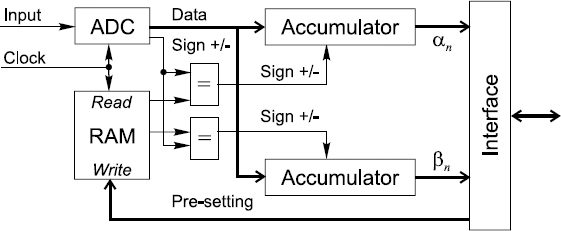
Figure 19.12 Block scheme of the bioimpedance signal preprocessor performing the signal demodulation and data compression functions

It follows from the description of the complexity-reduced DFT method given in Chapter 16 that this is especially attractive for applications where the spectrum of the signal to be analysed does not contain harmonics above the third (when system 1 is used) or the fifth (in the case of using system 2). Then the spectral estimations are actually single stage and no multiplication operations are executed. The conditions for bioimpedance analysis seem to fit this criterium. Multitone bioimpedance analysis might sometimes represent an exception, but at least the single carrier frequency analysis could be well implemented on the basis of this approach.

A number of benefits could be gained in this way. Firstly, the hardware for demodulation is simple. The basic scheme for estimation of Fourier coefficients is basically built on data accumulators. Secondly, real-time demodulation could be easily implemented on this basis by making estimation of the Fourier coefficients continuously on-line. Thirdly, due to the simplicity of the basic structure, multichannel demodulation could also be realized, which could be done in a sufficiently simple way. Fourthly, in addition, the approach is especially attractive for embedded bioimpedance analysers as they are characterized by low power consumption.

All of the mentioned considerations lead to the conclusion that demodulation of the bioimpedance signals can be arranged in accordance with the scheme given in Figure 19.12. Although Figure 19.12 illustrates the structure of a single-channel bioimpedance signal demodulator, the simple signal preprocessor shown there actually would be exactly the same in the case of a multi-channel demodulator. The ADC then has simply to be replaced by a multiplexer.

Note that estimates of the coefficients α_n and β_n rather than sample values of the modulated carrier are passed through the interface block to the computer. In this case these coefficients are equal to the corresponding Fourier coefficients a_n and b_n. Thus this very simple signal preprocessor performs the DFT and substantial data compression is achieved. This makes the task of the computer receiving these data much easier. It simply has to collect the preprocessed data and display the demodulated signals.

Bibliography

Artjuhs, J. and Bilinskis, I. (2006) Method and apparatus for alias suppressed digitizing of high frequency analog signals. EP 1 330 036 B1, European Patent Specification, Bulletin 2006/26, 28.06.2006.

Artyukh, Yu., Bilinskis, I., Greitans, M. and Vedin, V. (1997) Signal digitizing and recording in the DASPLab System. In Proceedings of the 1997 International Workshop on Sampling Theory and Application, Aveiro, Portugal, June 1997, pp. 357–60.

Artyukh, Yu., Bilinskis, I. and Vedin, V. (1999) Hardware core of the family of digital RF signal PC-based analyzers. In Proceeding of the 1999 International Workshop on Sampling Theory and Application, Loen, Norway, 11–14 August 1999, pp. 177–9.

Artyukh, J., Bilinskis, I., Boole, E., Rybakov, A. and Vedin, V. (2005) Wideband RF signal digititising for high purity spectral analysis. In Proceedings of the International Workshop on Spectral Methods and Multirate Signal Processing (SMMSP 2005), Riga, Latvia, 20–22 June 2005, pp. 123–8.

Artyukh, Yu., Boole, E. and Vedin, V. (2006) Digital synchronous demodulator for measurement of complex amplitude deviation. electronics and electrical engineering. Kaunas: Technologija, 5(69), 29–32.

Bilinskis, I. and Artjuhs, J. (2006) Method and apparatus for alias suppressed digitizing of high frequency analog signals. United States Patent US 7,046,183 B2, 16 May 2006.

Bilinskis, I. and Sadovskis, G. (1974) Statistical measurement of phase angles (in Russian). In Proceedings of Conference on Phasometric Systems and Devices, Tomsk, pp. 170–4.

Bilinskis, I., Trejs, P.P. and Nemirovski, R.F. (1972) Verfarhen zur digitalen Messung von Zeitintervallen und Einrichtung zu dessen Realisierung. Patentscrift 93960, DDR.

Bilinskis, I., Trejs, P.P. and Nemirovski, R.F. (1974) Zpusob digitalniho mereni casovych intervalu a zarizeni k provadeni tohoto zpusobu. Aut. osved. 163383, CSSR.

Min, M., Ollmar, S. and Gersing, E. (2003) Electrical impedance and cardiac monitoring – technology, potential and applications. International Journal of Bioelectromagnetism, 5(1), 53–6.