
15
DFT of Nonuniformly Sampled Signals
In the classical case of processing periodically sampled signals on the basis of the DFT, the results of the performed DFT reflect the structure of the respective signals in the frequency domain. In other words, the DFT of periodically sampled signals leads to signal decomposition and to obtaining their spectra. Therefore it is normal to expect that when the DFT of nonuniformly sampled signals are calculated the results will also represent the spectra of these signals. However, these expectations are typically not fulfilled. As soon as the sampling procedure is randomized, the DFT of the respective signals become strongly sampling-dependent. As explained in the previous chapter, the basis functions for the DFT under the conditions of nonuniform sampling become unorthogonal. If DFT could be performed as unorthogonal transforms then the preference should be given to such an approach. However, that is not always possible. Direct calculations of DFT have to be undertaken while clearly realizing that these transforms will not complete the process of signal decomposition into their components. Estimating the Fourier coefficients then actually leads to acquiring intermediate signal processing results containing valuable information. Therefore the outcome of the DFT under these conditions should not always be automatically regarded as spectrograms of the respective signals. Some comments on this are given in Section 15.1. To obtain spectrograms showing the signal components in the frequency domain, this information has to be additionally processed taking into account the mutual unorthogonality of the basis functions leading to cross-interference between the signal components being estimated. It is not a trivial matter. A lot of effort has been spent on research in this area and gradually several approaches to processing transformed nonuniformly sampled signals have been developed. Some of the methods and techniques used for this type of signal processing and their potential are discussed in this chapter.
It is worth paying a lot of attention to calculating raw DFT of nonuniformly sampled signals, as the estimates obtained in this way play a vital role in the subsequent digital processing of the transformed signals. Such DFT support all kinds of digital signal filtering and other signal processing procedures, including signal waveform reconstruction, and the quality of the final signal processing results often depends on the performance of the involved DFT.
15.1 Problems Related to Sampling Irregularities
To achieve the capability of processing signals in a broad frequency range not limited by half of the used sampling rate, sampling must be nonuniform. However, once the signal digitizing is based on nonuniform sampling, processing of the signals then has to be organized with the specifics of this technique taken into account. Apparently it is essential to obtain a clear insight into the details of processing this type of digital signal.
15.1.1 Alternative Approaches to DFT
General considerations of this have been given in Chapter 3. If the sampling point process satisfies condition (3.13), then it follows from Equation (3.14) that

This means that asymptotically there should be no bias error and the statistical estimation errors should tend to c2/N (c is the amplitude of the signal component being estimated). Therefore, for large N, interval systematic bias and statistical error at least should be small. That would be so if the side effect caused by the nonorthogonality of the basis functions and the cross-interference effect due to it did not exist. This effect certainly cannot be ignored. If these considerations are taken into account, the following randomized estimation schemes can be suggested:
- The signal x(t) is sampled pseudo-randomly at predetermined time instants {tk}. The values of cos(2πfitk) and sin(2πfitk) are calculated beforehand, stored in a memory and then later used for estimation. To reduce estimation errors to an acceptable level by averaging, a relatively large data block is processed. The errors due to the cross-interference remain, fact that has to be taken into account at further processing of the obtained raw estimates of the Fourier coefficients.
- The signal x(t) is sampled pseudo-randomly at predetermined instants {tk} and this timing information is exploited not only when calculating the corresponding set {sin(2πfitk), cos(2πfitk)} but also to compensate for errors due to the sampling irregularities.
The first approach is used most often and leads to satisfactory results if the DFT are carried out to obtain raw Fourier coefficient estimates used in the process of further calculations. The second estimation scheme, although much more complicated than the first one, is in principle more advanced. The mechanism of error reduction then is not averaging, and the number N of the sample values to be processed depends only on the complexity of the signal x(t) being processed, i.e. on the quantity of its components. Therefore it is applicable under more dynamic conditions for short-time estimations. Several methods for the DFT that belong to this category are discussed in this chapter in addition to the unorthogonal transform approach described in the previous chapter. However, before considering them, two possible techniques for estimating the Fourier coefficients are compared. One of the alternative techniques is based on direct calculations of the DFT and the second possible approach can be realized in accordance with the best-fitting procedure.
15.1.2 Best-fitting Procedure Versus Direct DFT
Consider an arbitrary frequency f and the following row of frequencies:
![]()
Apparently in the case where signals are sampled periodically these frequencies overlap. Suppose a monoharmonic signal with an amplitude equal to 1 and the frequency fi belonging to row (15.1) is randomly sampled at N sampling instants {tk}, so that the following digital signal is obtained:
![]()
As the sampling operation is randomized, the aliasing effect has to be eliminated or at least suppressed. The graphical interpretation of this effect is given in Figure 15.1. The sample values of x(tk) are shown as points. To find out how randomization of sampling helps to suppress aliasing, an attempt will be made to draw some other sinusoids with frequencies from row (15.1) through the indicated set of points. The outcome of such a best-fit operation strongly depends on the mode of applied sampling. The least mean square errors of drawing a sine wave at one of the frequencies fj from this row through the points{x(tk)} will be equal to zero only in the case of periodic sampling, as shown in Figure 15.1(a). Even a slight randomization of sampling will magnify this error considerably. With an increasing degree of sampling randomization, the error in drawing a sine wave at any of the frequencies (15.1) through the sample points tends to become more and more significant. This is illustrated by Figures 15.1(b) and (c). They show that at larger values of σ/μ the suppression of the alias is more noticeable.
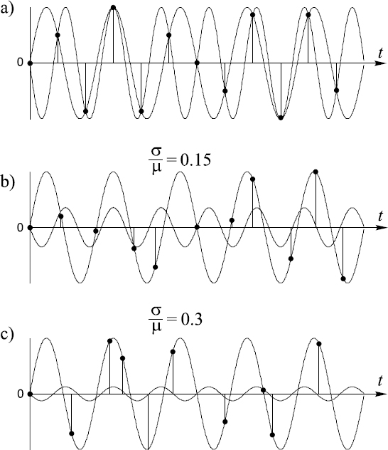
Figure 15.1 Suppression of an aliasing signal component in the case where the signal has been sampled nonuniformly
The effectiveness of the suppression of aliasing may be characterized by the ratio γji = Pj/Pi, where Pi and Pj are the mean powers of the sinusoids at the frequencies fi and fj respectively. The procedure of drawing a sinusoid at frequency fj through the sample points {x(tk)} with the least square error should be performed according to the following condition:

Estimates ãj and ![]() j of the Fourier coefficients characterizing the sinusoid at frequency fj drawn through the sample points with the least square error are obtained by solving the system of equations corresponding to Equation (15.2):
j of the Fourier coefficients characterizing the sinusoid at frequency fj drawn through the sample points with the least square error are obtained by solving the system of equations corresponding to Equation (15.2):
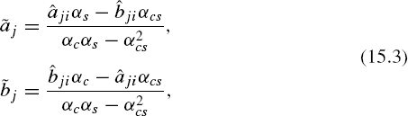
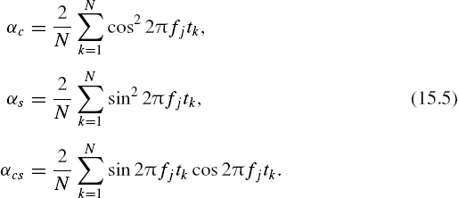
where

and
The solution to the minimization task allows the degree of aliasing γji to be defined as follows:
![]()
Now consider the notation in Equation (15.5). Obviously, αc ≅ 1 and interval αcs ≅ 0. This suggests that aliasing can also be evaluated by the following approximate equality:
![]()
Substitution of Equation (15.7) for Equation (15.6) is very desirable, because it considerably simplifies further analysis. The errors arising in this case were evaluated by computer simulations and they are small enough to justify this substitution. Therefore there is no need to use the more correct but computationally significantly more complicated best-fitting approach to estimate the Fourier coefficients. Direct calculations performed on the basis of Equation (14.1) provide good enough results.
Taking into account the random nature of sampling, aliasing should actually be characterized by the expected value:
![]()
15.1.3 Sample Values Partly Fitting to Any Frequency
This analysis confirms the already mentioned (see Chapter 9) conclusion that elimination of aliases cannot be achieved simply by direct substitution of the periodic sampling by randomization. While intensification of sampling randomization helps to reduce the amplitude of the aliasing frequency drawn through the sampling points of the true signal, the amplitude of the aliasing sinusoid, estimated on the basis of Equation (15.2), will not be zero even when there are no aliasing frequencies present. The least squares error of drawing an aliasing sinusoid through the sampling points of the true signal component depends on the specific irregularities of the involved sampling point process and the power of other signal components. Therefore randomization of sampling provides the necessary preconditions for effective elimination of aliasing. More elaborate specific anti-aliasing methods are needed and should be used to achieve complete elimination of the aliases. The interpretation suggested in Chapter 9 of aliasing processes taking place when processing randomly sampled signals called ‘fuzzy aliasing’ provides the key to resolution of this problem.
So far the discussion in this section has been focused on the anti-aliasing issue. Although the above mathematical expressions were derived for evaluation of inadequate suppression of aliases, they are also applicable for an analytical description of the best-fit operation in those cases where an attempt has been made to draw a sinusoid at any arbitrary frequency fj through a set of sample value points belonging to another sinusoid at a different frequency fi according to Equation (15.2). It is irrelevant that both of these frequencies belong to the row (15.1). The estimates of the Fourier coefficients defining the amplitude of this sinusoid at frequency fj depends on the parameters of other sinusoids at frequency fi and on the specific nonuniformities of the involved sampling point process. Actually a set of signal sample values, obtained at nonuniform sampling of a signal, partly fits to any frequency. It is emphasized that the best-fitting procedure as well as direct calculations of the Fourier coefficient estimates, working well in cases where signals are sampled periodically, do not provide sufficiently accurate representation of signals in the frequency domain whenever signals have been sampled nonuniformly. Actually the obtained DFT results then represent simply some kind of raw estimates of the Fourier coefficients. Nevertheless, they are often needed and have to be calculated at some stage of the complete signal processing process.
The given relationships are relevant also to the cross-interference effect related to the nonorthogonality of the nonuniformly sampled discrete basis functions.
15.2 Cross-interference Corrupting DFT
Deliberate randomization of sampling, while crucial for achieving the capability of alias-free processing of signals digitally in a wide frequency range, also leads to some problems. In particular, the basis functions for the DFT under conditions of nonuniform sampling become nonorthogonal, which leads to cross-interference between signal components. The impact of this cross-interference is observed as signal parameter estimation errors. They are both sampling and signal-dependent.
To find exactly how the cross-interference due to sampling nonuniformities impact on the process of the DFT, computer simulations of the DFT, performed under conditions of pseudo-randomized additive sampling, could be carried out. It is convenient to start this experiment by using at first a single tone variable frequency signal and a DFT filter tuned to frequency f1 for estimating the signal parameters at this frequency, specifically the Fourier coefficients, amplitude and phase. If the signal is sampled periodically, the performance of this filter would be close to ideal. Figure 15.2 illustrates the results obtained in this case. At the signal frequency fi = f1 the calculated values of the Fourier coefficient estimates (for growing amplitude of the signal) are close to their true values (as shown by the dashed line 1) and these estimates are near to zero for signal frequencies deviating from f1.
Now suppose that a single tone signal x(t) at frequency f1 is sampled nonuniformly and the Fourier coefficient a1 is estimated under the conditions where the signal phase is equal to π/2. Then b1 = 0 and the value of a1 is estimated as being equal to the signal amplitude if there are no estimation errors (line 1). However, under the conditions of this experiment, the sampling process is noticeably irregular, which leads to these errors. As shown in Figure 15.2, this error increases proportionally to the growing true value of a1 (line 2). In this particular case, â1 = a1 (A1C1), where the coefficient A1C1 is a constant indicating the strength of the impact of the sampling imperfections on the estimation of the coefficient a1.
Actually the behaviour of the filter is even more complicated. There are also noticeable estimation errors caused by nonuniform sampling of other signal components and these errors depend on the power and frequencies of these signal components. In fact, the irregularities of the sampling point stream leads to cross-interference between the signal components. This phenomenon can be observed if filtering of a nonuniformly sampled signal with two or more components is studied. It can be seen that each signal component impacts on the parameter estimation of all other signal components and that this impact directly depends on the specific nonuniformities present in the involved sampling process. To observe this phenomenon, the experiment should be repeated. Exactly the same sampling point process should be used for the signal sampling and a sine function at frequency fm should be added to the previously used cosine function with gradually increased amplitude. The results obtained in this case are displayed as line 3 in Figure 15.2. It can be seen that the presence of the irregularly sampled component at frequency fm adds to the estimation error. However, the value of the coefficient A1C1 remains the same; it is not changed by the second component. Therefore it seems that in this second case â = a (A1C1) + bm(A1Sm), where the coefficient A1Sm indicates the strength of the impact of the sinusoidal signal component at frequency fm on the estimation of the coefficient a1 when the signal is sampled in that particular way. The impact of the specific nonuniformities of the sampling point process can be characterized by constant coefficients. Thus it seems that these coefficients characterizing the cross-interference between the signal components might be introduced as follows:
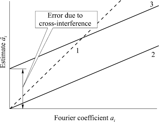
Figure 15.2 Illustration of the impact sampling irregularities on the errors when estimating the Fourier coefficients

These coefficients are actually the weights of the errors introduced by nonuniform sampling of the signal sine (or cosine) component at frequency fm that corrupts the estimation of a Fourier coefficient ai (or bi) at frequency fi. They are derived mathematically in Chapter 18. More detailed studies of this subject reveal that the description of the experiment given above reflects the involved relationships only approximately. A system of equations has to be composed and used for a more accurate description, as shown in Chapter 18. The usefulness of the introduced interference coefficients is demonstrated there by showing how this concept could be exploited for adapting alias-free processing of signals to the sampling nonuniformities.
15.3 Exploitation of FFT
Performing the DFT requires a lot of calculations. To reduce the number of involved multiplication operations, fast algorithms are widely used, especially the FFT. However, the existing fast algorithms have been developed on the assumption that the intervals between signal sample values are constant. Therefore, in general, they cannot also be directly used for processing nonuniformly sampled signals. Nevertheless, if the nonuniform sampling is performed as a pseudo-randomized procedure, under certain conditions it is possible to exploit the FFT for reduction of the computational complexity of the DFT, and that could be done relatively often. Different approaches to this problem have to be used to handle digital signals formed on the basis of either directly or indirectly randomized sampling discussed in Chapters 6 and 7 respectively.
15.3.1 Application of FFT for Processing Nonuniformly Sampled Signals
To process the directly randomized nonuniformly sampled signals by using algorithms developed for processing periodically amplitude-sampled signals, the so-called zero padding method is typically used. According to this method, zeroes are inserted into the nonuniform signal sample value sequence at those periodically repeating time instants where there are no signal sample values, so that the sampling process is transformed into a periodic one. However, zero padding is a crude method and its application leads to the introduction of substantial errors. Indeed, each zero replaces a signal sample value when this technique is used, which means that each substitution of this kind introduces a particular instantaneous error equal to the respective missing sample value. If there is a large quantity of this kind of error then the spectrograms obtained are naturally of a poor quality. Whether it is acceptable or not depends on the proportion between the sampling slots filled by the signal sample values and the empty slots marked as zeroes. The achievable performance is illustrated in Figure 15.3 where spectrograms obtained at various sample value/zero ratios are displayed.
It can be seen that the zero padding procedure and application of the FFT leads to a more or less significant distortion of the spectrograms depending on the specific sample value/zero ratios. In the cases of Figures 15.3(b) and (c) half and two-thirds of the sample values are randomly replaced by zeroes respectively. These spectrograms can be compared with the true signal spectrogram obtained under conditions of correct periodic sampling and are displayed in Figure 15.3(a). Obviously zero padding has led to the introduction of substantial errors.
The idea of using the FFT to obtain estimates of the Fourier coefficients is of course attractive, as application of this fast algorithm drastically reduces the amount of calculations. However, using this approach evidently leads to large errors in estimating the Fourier coefficients. The achievable accuracy of these estimates is typically not acceptable. Therefore this procedure, if and when used, should be regarded as a preliminary calculation providing only raw intermediate results. The degree of its usefulness depends on the specific algorithm used for signal analysis.
The algorithm for signal spectrum analysis and waveform reconstruction considered in Chapter 20 confirms the fact that such usage of the FFT makes sense and could lead to good results. This algorithm is focused on the realization of an obvious idea that a priori information should be used as often as possible. To achieve that, the initially inserted zeroes at some processing stage should be replaced by approximate estimates of the signal sample values roughly estimated as a result of the FFT. It is shown that this leads to a dramatic reduction in the mentioned errors. Even better results are obtained when an iterative procedure of spectral analysis and waveform reconstruction is used. In is case the missing uniform sample values are substituted first by zeroes, then estimated signal values are inserted in those places and after that even more accurately estimated signal sample values are used. That leads to a significant improvement in the estimation accuracy. Such an approach makes it possible to rationalize signal processing on the basis of the FFT.

Figure 15.3 Spectrograms obtained by using the FFT in the case where a signal is sampled pseudo-randomly and zeroes are inserted to regularize the sequence of the sample values
This specific example, considered in more detail in Chapter 20, demonstrates the fact that under certain conditions it is possible to use already existing fast algorithms, first of all the FFT, for an alias-free estimation of nonuniformly sampled wideband signal parameters in the frequency domain and for subsequent waveform reconstruction carried out on the basis of the inverse FFT. The fact is noteworthy as it suggests that probably there are also some other possibilities still not discovered of using fast algorithms that are effectively applicable for processing nonuniformly sampled signals.

Figure 15.4 Regularization of the sampling operation based on sine-wave crossings
15.3.2 Fast Transforms of Signals Sampled at Sine-Wave Crossing Instants
To achieve the applicability of the standard DSP computer programs for processing nonuniform digital signals, the representation of these signals apparently must be somehow regularized. Some varieties of nonuniform sampling techniques could be regularized more easily than others. The sampling method based on sinewave crossings, discussed in Chapter 7, might be considered as belonging to the first category as the specifics of this kind of sampling are typically favourable for regularization. Firstly, the nonuniformity of the sampling operation in this case is just a consequence of the specific signal sample value encoding based on timing of the signal and the reference waveform crossings. The irregularities observed with this type of sampling just occur; they are not introduced intentionally to achieve some desirable effect like suppression of the aliases. Secondly, it helps that the frequencies of the signals being sampled are usually below half of the mean sampling rate. The approach to regularization of the sampled signals in this case is simple and is illustrated in Figure 15.4.
The signal sample values {xk} are taken at the signal and the reference sinewave crossing instants, as shown in Figure 15.4(a). To regularize this type of sampling, all signal sample values should be assigned to the time instants tk, k = 0, 1, 2,..., which actually are the instants when the reference sine wave crosses the zero or some other constant level. Thus this regularization approach is simple and straightforward and leads naturally to the introduction of some noise ∊(tk). The signal values at these time instants differ from those corresponding to the signal reference function crossing instants. As shown in Figure 15.5, the value of a particular error ∊k depends on the angle of the signal/sine-wave crossing and on the time interval Δt between this crossing instant and the reference function zero-crossing instant tk. The fact that the time interval Δt is smaller for smaller values of the sampled signal helps to keep the relative errors close to a constant level for small to medium signal values.

Figure 15.5 Regularization error occurring as a result of ascribing the signal instantaneous value xk to the reference function zero-crossing instant
When the sampling results are regularized as explained, most of the classic DSP algorithms, including the fast ones like the FFT, could be used for processing the digital signals obtained in this way. However, the errors introduced at the sampling result regularization impose some limitations on the applicability of this approach. To assess these limitations, it is shown in Figure 15.6 how the power of the regularization noise ∊(tk) depends on the reference sine-wave frequency. Actually, the given curve is pessimistic as it has been calculated to conditions that are near to the worst. Specifically, the regularization errors ∊k were calculated for a full amplitude single-tone signal at the frequency just below the Nyquist limit. The time intervals Δt and the related regularization errors ∊k then tend to their maximal values.

Figure 15.6 Mean power of the regularization noise versus normalized reference sine-wave frequency
These estimation errors ∊k were calculated under the sampling conditions emulating the specifics of massive data acquisition from a variable number of signal sources. Specifically, the power of the regularization errors ∊k are given in Figure 15.6 for the case where the single tone signal is characterized by frequency fs and amplitude A. The mean sampling rate fms depends both on the reference frequency fr and the number n of signal sources as fms = fr/n. In this case the errors ∊k are calculated for various values of n while the mean sampling rate fms is kept constant and equal to 2.18753 fx. To keep the mean sampling rate fms constant, the reference frequency fr is appropriately changed for each n value. Note that n is equal to the reference frequency normalized with regard to the mean sampling rate n = fr/fms. This means that the power P∊ of the regularization noise ∊(tk), given for the growing numbers of signal sources, also indicates its dependence on the normalized reference frequency.
It can be seen from the diagram obtained and displayed in Figure 15.6 that the mean power of the regularization noise, even in the worst case, decreases quickly at relatively small numbers n of the signal sources encoded in this way. It seems that in many cases of data acquisition from multiple signal sources that the regularization approach should be applicable if the number is about 10 and more. The feasibility and rationale of this approach is further illustrated in Figure 15.7.
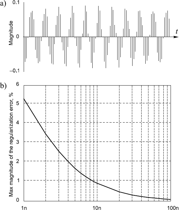
Figure 15.7 Illustration of (a) the digital regularization noise and (b) the maximal value of the regularization errors versus the normalized reference sine-wave frequency (number of signal sources) of the nearly worst case of sine-wave crossing sampling of a single-tone signal at a frequency close to the Nyquist limit
The digital regularization noise is shown in Figure 15.7(a) and the maximal value of the regularization errors versus the normalized reference sine-wave frequency (number of signal sources) is given in Figure 15.7(b).
The regularization noise ∊(tk) impacts on the processing of signals sampled on the basis of the sine-wave crossing approach like any other additive noise present in the signal. Figure 15.8 illustrates the impact of this noise on the estimation of a Fourier coefficient. To realize conditions under which the impact of regularization errors ∊k is most damaging, the errors in estimating the Fourier coefficients were calculated for a full amplitude single-tone signal at a frequency close to the Nyquist limit. The estimation errors were again calculated for the varying normalized reference frequency or, what is the same, for the varying number of signal sources.

Figure 15.8 Impact of the sampling regularization on the estimation of the amplitude of a single-tone signal.
The given curve corresponds to the nearly worst case. Errors corrupting the estimation of more complex signal parameters containing components at other lower frequencies are below the given curve. It can be seen from Figures 15.7 and 15.8 that even relatively small increases in the normalized reference frequency significantly reduce the noise ∊(tk) caused by the regularization procedure and the negative effects due to it. As a result the impact of the sampling regularization on the signal processing results is insignificant in a large area of the normalized reference frequency. The errors due to the nonuniform sampling regularization in the case where this particular sampling technique is used for remote sampling at massive data acquisition from many signal sources become insignificant when the number n of the signal sources exceeds 5 to 10. Therefore the errors related to the considered procedure of sampling regularization under the conditions typical for data acquisition from a large number of signal sources can often be ignored. This fact leads to the following conclusion:
If the remote sampling operations carried out in the process of massive data acquisition are performed on the basis of sine-wave crossings, the digital signals obtained in this way can usually be regularized and presented as periodically sampled signals even at relatively small numbers of signal sources (about 10 or more). Consequently, most of the well-developed traditional DSP algorithms for processing periodically sampled signals are applicable for processing digital signals reconstructed from the data acquired in this way from a relatively large quantity of remote signal sources.
15.4 Revealing the Essence of the Fourier Coefficient Estimation
There is no doubt that the Fourier transform plays a significant role in various algorithms for signal processing. Therefore it is crucial to perform this transform and use the results correctly. While the use of the DFT for dealing with periodically sampled signals is a well-established routine, the involved estimation of the Fourier coefficients becomes more problematic whenever the signal to be transformed is represented by the sequence of its sample values obtained in the process of randomized sampling. Therefore the conditions under which the estimates of the Fourier coefficients are calculated should be well understood. Unfortunately they are estimates of a parameter calculated for a given set of data, which makes the use of them obscure. Often it is much better to use the approach introduced in Section 8.3, based on the representation of the DFT by cumulative sums. The point is that this approach makes it possible to observe the estimation of the Fourier coefficients as a process. This subject will now be expanded.
The DFT performed in the course of Fourier analysis actually represents estimation of a spectral parameters aa or ba characterizing a signal x(tk) = xk at a given frequency fa. According to definition,

Calculations carried out according to these equations only provide the numerical values of the estimates âa and ![]() a. This kind of DFT might be considered as selective digital filtering. Application of such filters for signal decomposition and spectral analysis is quite popular. Their frequency response is given in Figures 15.9 and 15.10 just as a reference for further analysis of various aspects of this type of filtering.
a. This kind of DFT might be considered as selective digital filtering. Application of such filters for signal decomposition and spectral analysis is quite popular. Their frequency response is given in Figures 15.9 and 15.10 just as a reference for further analysis of various aspects of this type of filtering.
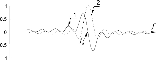
Figure 15.9 Frequency responses of the selective DFT filters for extracting the quadrature components of the signal.
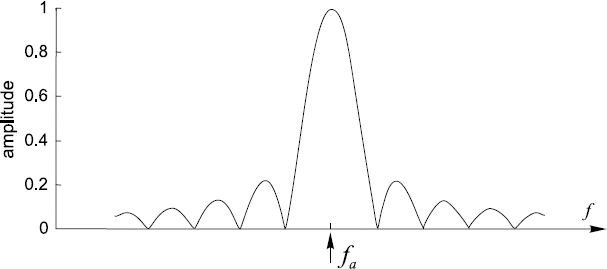
Figure 15.10 Typical amplitude–frequency response of a DFT filter
This kind of filtering will now be considered from a different angle. It can be seen from the expressions (15.10) that these coefficients are obtained by averaging the accumulated products of signal sample values each multiplied by the sample values of sine or cosine functions of a particular frequency taken at the same instants as the respective signal sample values. This accumulation process is stopped when a predetermined number N of sample values has been used. The Fourier coefficients are obtained as the end result of this accumulation process. No attention is paid to that process itself.
As pointed out in Chapter 8, the cumulative process is highly informative and substantially more information can often be extracted if this kind of spectral estimation is observed as a process. So far this approach has been used only for analysis of the effects from phase shifting of a periodic sampling point process. The proposed exploitation of the cumulative process has proved to be an efficient tool for discovery of well-hidden relationships. This fact has been confirmed by demonstration of the compensation effect that takes place when properly phase-shifted periodic sampling point processes are used. Now it will be shown that analysis of this sort of cumulative sum forming is often productive and useful. Emphasis is put on the application of this approach to the resolution of various signal filtering tasks.
The cumulative sums related to the Fourier transform can be given as

where fa is the frequency to which this type of DFT filter is tuned.
The calculation and use of these cumulative sums makes it possible to observe estimation of a Fourier coefficient as a process depending both on the signal being analysed and on the sampling point process used. Observation and analysis of these processes leads to the ability to obtain additional information.
The properties of these cumulative sums will now be described, starting with a case where the signal being filtered is given as
![]()
In this particular case the cumulative sums become

The properties of these functions depend on the frequencies f0 and fa and on the sampling point stream. Naturally, they are determined more easily in the case of periodic sampling. The cumulative sums shown in Figure 15.11 have been obtained for the coefficients a(f0) for various values of the frequencies f0 and fa. Note that in the case where f0 ≠ fa the value of the Fourier coefficient differs if it is estimated for various values of N.
It can be seen that these cumulative sums are quite informative. By observing them, it is possible to obtain more information about the involved signals than by just calculating the values of the corresponding Fourier coefficients. Therefore it often makes sense to use them in order to reveal the essence of various processes. It is easier to achieve that if it is clear what various shapes of these functions mean. Some typical cumulative sums obtained under specific conditions are shown in Figure 15.12.

Figure 15.11 Cumulative sums for various locations of frequencies f0 with respect to the central filter frequency fa in the case where the difference between them is relatively small
The given examples show typical cumulative sums for the case of a single tone signal. The signal structure that might be expected in reality is of course much more complicated. Nevertheless, much can be learnt from observations of this kind of typical cumulative sum. First of all, the cumulative sum for a signal component at a frequency equal to the frequency to which the respective DFT filter is tuned graphically looks like a linearly increasing function. Therefore the presence of a linearly increasing component in a cumulative sum is evidence that the signal contains a component at the frequency of DFT filtering. This fact has been used before in Chapter 8 to demonstrate the alias compensation effect.
However, in general the analysis of these cumulative sums might prove not to be so simple. Apparently it has to cover cases where signals are composed from multiple components. Figure 15.13 illustrates the forming and analysing of cumulative sums in the case of multifrequency signals containing four components at the indicated frequencies.

Figure 15.12 Cumulative sums for both Fourier coefficients calculated for various locations of frequencies f0 with respect to the central filter frequency fa in the case where the signal phase angle ϕ = 45°

Figure 15.13 Example of (a) a multifrequency signal filtered by (b) a DFT filter tuned to the frequency of the first signal component in its spectrum
An ideal selective filter would filter out just one of these components. It would filter out the component at the frequency equal to the frequency at which the filter is tuned. In terms of cumulative sums, this component forms the linear increasing function 1 shown in Figure 15.14. The values indicate the amplitude of the corresponding component with the number N of signal samples taken into account. All other signal components would have to be filtered out. In reality the DFT filter only weakens their impact. These components form the particular cumulative sums 2, 3 and 4. The resulting cumulative sum 5 provides the result for the conventional DFT. The difference between the cumulative sums 1 and 5 represents the DFT errors. Two particular errors for N = 512 and N = 1024 are indicated. It is shown that there might be even bigger errors taking place at different N values. This example also shows what has to be achieved to improve DFT filtering. In fact, only the linear component of the total cumulative sum needs to be preserved. All other oscillating components have to be taken out.
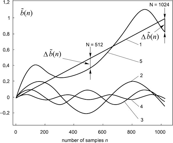
Figure 15.14 Cumulative sums formed for the multifrequency signal given in Figure 15.13
Attention should be drawn to the essential point that the traditional digital filtering methods could be used for processing or special filtering of the cumulative sums as the discrete argument (the sample-taking instants) in this case is regular. It is true that there are pseudo-random skips of the sampling instants, but each sampling event is placed on a regular grid. While filtering of the signal sample value sequences require application of special techniques as the sampling intervals are nonuniform, transformation of the task to filtering of cumulative sums leads to regularization of the filtering. This is a significant fact and can be exploited in various ways in order to increase the accuracy of signal transforms from time to frequency domains.
Note that the necessity to process signals in this way comes from the fact that the frequency response of the DFT filter is not ideal. It has side lobes. The usual approach used to reduce the harmful effects due to them is based on windowing. The described approach based on application of cumulative sums represents an alternative to application of the windowing techniques.
Bibliography
Allay, N. and Tarczynski, A. (2004) Spectral magnitude and phase estimation of digitally modulated signals from their nonuniform samples. In Proceedings of the IASTED International Conference on Communications Systems and Networks (CSN 2004) Marbella, Spain, 1–3 September 2004, pp. 237–42.
Bilinskis, I. and Mikelsons, A. (1992) Randomized Signal Processing. Prentice-Hall International (UK) Ltd.
Bland, D. M., Laakso, T. and Tarczynski, A. (1996) Analysis of algorithms for nouniform-time discrete Fourier transform. In International Symposium on Circuits and Systems (ISCAS'96), Vol. 2, Atlanta, Georgia, 12–15 May 1996, pp. 453–6.
Bland, D. M., Laakso, T. and Tarczynski, A. (1996) Application of NUT-DFT for reasampling nonuniformly sampled signals. In Proceedings of the Third IEEE International Conference on Electronics, Circuits, and Systems (ICECS'96), Vol. 1, Rhodos, 13–16 October 1996, pp. 586–9.
Bland, D.M., Tarczynski, A. and Laakso, T.I. (1996) Spectrum analysis of nonuniformly sampled signals using the NUT-DFT. In Proceedings of the IEEE Nordic Signal Processing Symposium NORSIG'96, Vol. 1, Helsinki, 24–27 September 1996, pp. 307–10.
Tarczynski, A. (2002) Spectrum estimation of nonuniformly sampled signals. In Proceedings of the 14th International Conference onDigital Signal Processing(DSP2002), Vol. 2, Santorini, Greece, 1–3 July 2002, pp. 795–8. 7504-1.
Tarczynski, A. and Allay, N. (2003) Digital alias-free spectrum estimation of randomly sampled signals. In the 7th World Multi-Conference on Systemics, Cybernetics and Informatics (SCI'03), Vol. IV, Orlando, Florida, 27–30 July 2003, pp. 344–8.
Tarczynski, A. and Allay, N. (2004) Spectral analysis of randomly sampled signals: suppression of aliasing and sampler jitter. IEEE Trans. on Signal Processing, 52 (12), December, 3324–34.
Tarczynski, A., Bland, D. M. and Laakso, T. (1996) Spectrum estimation of non-uniformly sampled signals. In Proceedings of the IEEE International Symposium on Industrial Electronics (ISIE'96), Vol. 1, Warsaw, 17–20 June 1996, pp. 196–200.
Tarczynski, A. and Valimaki, V. (1996) Modifying FIR and IIR filters for processing signals with lost samples. In Proceedings of the IEEE Nordic Signal Processing Symposium (NORSIG'96), Vol. 1, Helsinki, 24–27 September 1996, pp. 359–62.