11

Micro-programmed Adaptive Filtering Applications

11.1 Introduction

Deterministic filters are implemented in linear and time-invariant systems to remove out-of-band noise or unwanted signals. When the unwanted signals are known in terms of their frequency band, a system can be designed that does not require any adaptation in real time. In contrast, there are many scenarios where the system cannot be deterministically determined and is also time-variant. Then the system is designed as a linear time-invariant (LTI) filter in real time and, to cater for time variance, the filter has to update the coefficients periodically using an adaptive algorithm. Such an algorithm uses some error-minimization criterion whereby the output is compared with the desired result to compute an error signal. The algorithm adapts or modifies the coefficients of the filter such that the adapted system generates an output signal that converges to the desired signal [1, 2].

There are many techniques for adaptation. The selection of an algorithm for a particular application is based on many factors, such as complexity, convergence time, robustness to noise, ability to track rapid variations, and so on. The algorithm structure for effective implementation in hardware is another major design consideration.

11.2 Adaptive Filter Configurations

Adaptive filters are used in many settings, some of which are outlined in this section.

11.2.1 System Identification

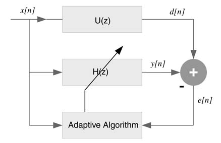
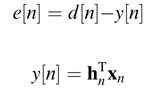
The same input is applied to an unknown system U(z) and to an adaptive filter H(z). If perfectly identified, the output y[n] of the adaptive filter should be the same as the output d[n] of the unknown system. The adaptive algorithm first computes the error in the identification as e[n] = d[n] – y[n]. The algorithm then updates the filter coefficients such that the error is minimized and is zero in the ideal situation. Figure 11.1 shows an adaptive filter in system identification configuration.

Figure 11.1 Adaptive filter in system identification configuration

11.2.2 Inverse System Modeling

The adaptive filter H(z) is placed in cascade with the unknown system U(z) . A known signal d[n] is periodically input to U (z) and the output of the unknown system is fed as input to the adaptive filter. The adaptive filter generates y[n] as output. The filter, in the ideal situation, should cancel the effect of U (z) such that H (z)U(z) =1. In this case the output perfectly matches with a delayed version of the input signal. Any mismatch between the two signals is considered as error e[n]. An adaptive algorithm computes the coefficients such that this error is minimized. This configuration of an adaptive filter is shown in Figure 11.2

This configuration is also used to provide equalization in a digital communication receiver. For example, in mobile communication the signal transmitted frogman antenna undergoes fading and multi-path effects on its way to a receiver. This is compensated by placing an equalizer at the receiver. A know input is periodically sent by the transmitter. The receiver implements an adaptive algorithm that updates the coefficients of the adaptive filter to cancel the channel effects.

11.2.3 Acoustic Noise Cancellation

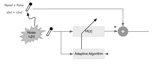
An acoustic noise canceller removes noise from a speech signal. A reference microphone also picks up the same noise which is correlated with the noise that gets added in the speech signal. An adaptive filter cancels the effects of the noise from noisy speech. The signal v₀[n] captures the noise from the noise source. The noise in the signal v₁[n] is correlated with v₀[n], and the filter H(z) is adapted to produce an estimate of v₁[n], which is then cancelled from the signal x[n], where x[n] = s[n] + v₁[n] and s[n] is the signal of interest [3, 4]. This arrangement is shown in Figure 11.3.

Figure 11.2 Adaptive filter in inverse system modeling

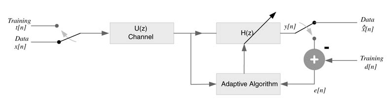
Figure 11.3 Acoustic noise canceller

11.2.4 Linear Prediction

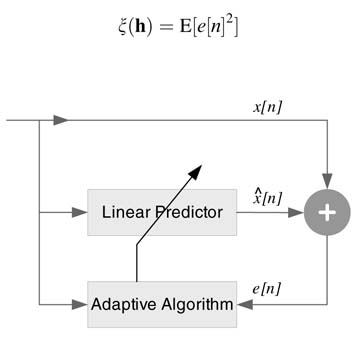
Here an adaptive filter is used to predict the next input sample. The adaptive algorithm minimizes the error between the predicted and the next sample values by adapting the filter to the process that produces the input samples.

An adaptive filter in linear prediction configuration is shown in Figure 11.4. Based on N previous values of the input samples, x[n – 1], x[n – 2],…, x[n –N], the filter predicts the value of the next sample x[n] as x^[n ]. The error in prediction e[n] =x[n] – x^{^}[n] is fed to an adaptive algorithm to modify the coefficients such that this error is minimized.

11.3 Adaptive Algorithms

11.3.1 Basics

An ideal adaptive algorithm computes coefficients of the filter by minimizing an error criterion ξ (h). The criterion used in many applications is the expectation of the square of the error or mean squared error:

Figure 11.4 Adaptive filter as linear predictor

where h _n= h_n[0], h_n[1], h_n[2],… , h_n[N– 1 ] and x_n= x[n], x[n – 1], x[n – 2],…, x[n –(N– 1)]. Using these expressions, the mean squared error is written as:

Expanding this expression results in:

The error is a quadratic function of the values of the coefficients of the adaptive filter and results in a hyperboloid [1]. The minimum of the hyperboloid can be found by taking the derivative of_ļ ξ (h) with respect to the values of the coefficients. This results in:

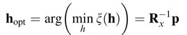
where R_x= E[x_n x^T_n ] and p= E[d[n] x_n].

Computing the inverse of a matrix is computationally very expensive and is usually avoided. There are a host of adaptive algorithms that recursively minimize the error signal. Some of these algorithms are LMS, NLMS, RLS and the Kalman filter [1, 2].

The next sections present Least Mean Square (LMS) algorithms and a micro-programmed processor designed around algorithms.

11.3.2 Least Mean Square (LMS) Algorithm

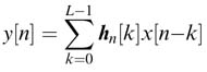
This is one of the most widely used algorithms for adaptive filtering. The algorithm first computes the output from the adaptive filter using the current coefficients from convolution summation of:

(11.1)

The algorithm then computes the error using:

(11.2)

The coefficients are then updated by computing a new set of coefficients that are used to process the next input sample. The LMS algorithm uses a steepest-decent error minimization criterion that results in the following expression for updating the coefficients [1]:

(11.3)

The factor µ determines the convergence of the algorithm. Large values of µ result in fast convergence but may result in instability, whereas small values slow down the convergence. There are algorithms that use variable step size for µ and compute its value based on some criterion for fast conversion [5, 6].

The algorithm for every input sample first computes the output y[n] using the current set of coefficients h_n[k], and then updates all the coefficients using (11.3).

11.3.3 Normalized LMS Algorithm

The main issue with the LMS algorithm is its dependency on scaling of x[n] by a constant factor µ .An NLMS algorithm solves this problem by normalizing this factor with the power of signal to noise ratio (SNR) of the input signal. The equation for NLMS is written as:

(11.4)

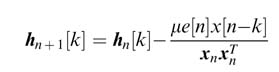
The step size is controlled by the power factor x_n x^T_n . If this factor is small, the step size is set large for fast convergence; if it is large, the step size is set to a small value [5, 6].

11.3.4 Block LMS

Here, the coefficients of the adaptive filter are changed only once for every block of input data, compared with the simple LMS that updates on a sample-by-sample basis. A block or frame of data is used for the adaptation of coefficients [7]. Let N be the block size, and h_{n– N} is the array of coefficients computed for the previous block of input data. The mathematical representation of the block LMS is presented here.

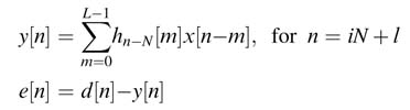
First the output samples y[n] and the error signal e[n] are computed using h_{n – N} for the current block i of data for l = 0,…, N –1:

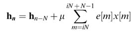
Using the error signal and the block of data, the array of coefficients for the current block of input data is updated as:

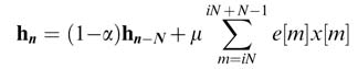
In the presence of noise, a leaky LMS algorithm is sometimes preferred for updating the coefficients. For 0< α< 1, the expression for the algorithm is:

11.4 Channel Equalizer using NLMS

11.4.1 Theory

A digital communication receiver needs to cater for the impairments introduced by the channel. The channel acts as U(z) and to neutralize the effect of the channel an adaptive filter H(z) is placed that works incascade with the unknown channel and the coefficients of the filter are adapted to cancel the channel effects. One of the most challenging problems in wireless communication is to device algorithms and techniques that mitigate the impairments caused by multi-path fading effects of a wireless channel. These paths result in multiple and time-delayed echoes of the transmitted signal at the receiver. These delay spreads are up to tens of microseconds and result in inter-symbol interference spreading over many data symbols. To cater for the multi-path effects, either multi-carrier techniques like OFDM are used, or single sarrier (SC) techniques with more sophisticated time and frequency equalizations are performed.

A transmitted signal in a typical wireless communication system can be represented as:

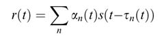
where s_b(t) and s(t) are baseband and passband signals, respectively, and f_c is the carrier frequency. This transmitted signal goes through multiple propagation paths and experiences different delays τ _n (t) and attenuation α _n (t) while propagating to a receiver antenna. The received signal at the antenna is modeled as:

There are different channel models that statistically study the variability of the multi-path effects in a mobile environment. Rayleigh and Ricean fading distributions [10–13] are generally used for channel modeling. A time-varying tap delay-line system can model most of the propagation environment. The model assumes L multiple paths and expresses the channel as:

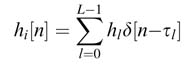
where h_l and τ _l are the complex-valued path gain and the path delay of the l th path, respectively. There are a total of L paths that are modeled for a particular channel environment.

The time-domain equalizer implements a transversal filter. The length of the filter should be greater than the maximum delay that spreads over many symbols. In many applications this amounts to hundreds of coefficients.

11.4.2 Example: NLMS Algorithm to Update Coefficients

This example demonstrates the use of an NLMS algorithm to update the coefficients of an equalizer. Each frame of communication appends a training sequence. The sequence is designed such that it helps in determining the start of a burst at the receiver. The sequence can also help in computing frequency offset and an initial channel estimation. This channel estimation can also be used as the initial guess for the equalizer. The receiver updates the equalizer coefficients and the rest of the data is passed through the updated equalizer filter. In many applications a blind equalizer is also used for generating the error signal from the transmitted data. This equalizer type compares the received symbol with closest ideal symbol in the transmitted constellation. This error is then used for updating the coefficients of the equalizer.

In this example, a transmitter periodically sends a training sequence t[n], with n = 0… N_t–1, for the receiver to adapt the equalizer coefficients using the NLMS algorithm. The transmitter then appends the data d[n] to form a frame. The frame consisting of data and the training is modulated using QAM modulation technique. The modulated signal is transmitted. The signal goes through a channel and is received at the receiver. The algorithm first computes the start of the frame. A training sequence is selected that helps in establishing the start of the burst [12]. After marking the start of the frame, the received training sequence helps in adapting the filter coefficients. The adaption is continued in blind mode on transmitted data. In this mode, the algorithm keeps updating the equalizer coefficients using knowledge of the transmitted signal. For example, in QAM the received symbol is mapped to the closest point of the constellation and the Euclidian distance of the received point from the closest point in the constellation is used to derive the adaptive algorithm.

The error for the training part of the signal is computed as:

where t[n] and t_r[n] are the transmitted and received training symbol, respectively. For the rest of the data the equalizer works in blind mode and the error in this case is the distance between the received and the closest symbols d[n] and d_r[n], resepectively:

The MATLAB^® code implementing an equalizer using an NLMS algorithm is given here:

Figure 11.5 Equalizer example. (a) Unequalized received signal. (b) Equalized QAM signal at the receiver

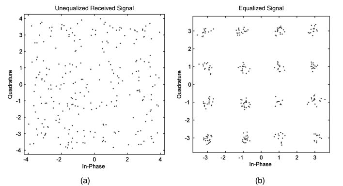
Figure 11.5 shows a comparison between an unequalized QAM signal and an equalized signal using the NLMS algorithm.

Usually divisions in the algorithm are avoided while selecting algorithms for implementation in hardware. For the case of NLMS, The Newton Repson method can be used for computing 1/x _n x _n ^T. Modified MATLAB^® code of the NLMS loop of the implementation is given here:

To avoid division a simple LMS algorithm can be used. For the LMS algorithm, the equation for updating the coefficients need not perform any normalization and the MATLAB^® code for adaptation is given here:

for i=MAX_SPREAD:Length_Training
 xn=Training_Data(i:-1:i-MAX_SPREAD+1);
 y(i)=xn*hn;
 d(i)=Training(i);
 e(i)=d(i)-y(i);
 hn = hn + mue*e(i)*xn’;
 end

11.5 Echo Canceller

An echo canceller is an application where an echo of a signal that mixes with another signal is removed from that signal. There are two types of canceller, acoustic and line echo.

11.5.1 Acoustic Echo Canceller

In a speaker phone or hands-free mobile operation, the far-end speaker voice is played on a speaker. Multiple and delayed echoes of this voice are reflected from the physical surroundings and are picked up by the microphone along with the voice of the near-end speaker. Usually these echo paths are long enough to cause an unpleasant perception to the far-end speaker. An acoustic echo canceller is used to cancel the effects. A model of the echo cancellation problem is shown in Figure 11.6.

Considering all digital signals, let u[n] be the far-end voice signal. The echo signal is r[n] and it gets added in to the near-end voice signal x[n]. An echo canceller is an adaptive filter h[n] that ideally takes u[n] and generates a replica of the echo signal, r ^ [n]. This signal is cancelled from the received signal to get an echo-free signal, x^[n], where:

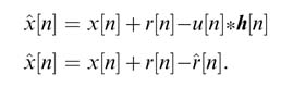
Figure 11.6 Model of an acoustic echo canceller

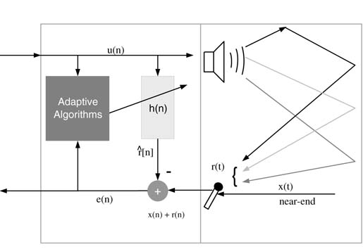
Figure 11.7 Line echo due to impedance mismatch in the 4:2 hybrids at the central office and its cancellation in Media Gateway

To cancel a worst echo path of 500 milliseconds for a voice sampled at 8 kHz requires an adaptive filter with 4000 coefficients. There are several techniques to minimize the computational complexity of an echo canceller [13–15].

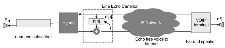
11.5.2 Line Echo Cancellation (LEC)

Historically, most of the local loops in telephony use two wires to connect a subscriber to the central office (CO). A hybrid is used at the CO to decouple the headphone and microphone signals to four wires. A hybrid is a balanced transformer and cannot be perfectly matched owing to several physical characteristics of the two wires from the subscriber’s home to the CO. Any mismatch in the transformer results in echo of the far-end signal going back with the near-end voice. The phenomenon is shown in Figure 11.7. The perception of echo depends on the amount of round-trip delay in the network.

The echo is more apparent in Vo IPasthere are some inherent delays in processing the compressed voicesignal that are accumulate dover buffering and queuing delay sate very hop of the IP network. In a VoIP network the delay scan build up to120–150 ms.This makes the round trip delay around300 ms. It is therefore very critical for VoIP applications to cancel out any echo coming from the far end [16].

A line echo cancellation algorithm detects the state in which only far-end voice is present and the near-end is silent. The algorithm implements a voice-activity detection technique to check voice activity at both ends. This requires calculating energies on the voice received from the network and the voice acquired in a buffer from the microphone of the near end speaker. If there is significantly more energyin the buffer storing the voice from the network compared with the buffer of voice from the near-end microphone, this infers the near-end speech buffer is just stori the echo of the far-end speech and the algorithm switches to a state that updates the coefficients. The algorithm keeps updating the coefficients in this state. The update of coefficients is not performed once the near-end voice is detected by the algorithm or double-talk is detected (meaning that the voice activity is present at both near and far end). In all cases the filtering is performed for echo cancellation.

The LEC requirements for carrier-class VoIP equipment are governed by ITU standards such as G.168 [17]. The standard includes a rigorous set of tests to ensure echo-free call if the LEC is complianttothe standard. The standard also has many echo path models that help in the development of standard compliant algorithms.

11.6 Adaptive Algorithms with Micro-programmed State Machines

11.6.1 Basics

It is evident from the discussion so far in this chapter that, although coefficient adaptation is the main component of any adaptive filtering algorithm, several auxiliary computations are required for complete implementation of the associated application. For example, for echo cancelling the algorithm needs first to detect double-talk to find out whether coefficients should be updated or not. The algorithms for double-talk detection are of a very different nature [18–20] than filtering or coefficient adaptation. In addition the application also requires decision logic to implement one or the other part of the algorithm. All these requirements favor a micro-programmed accelerator to implement. This also augments the requisite flexibility of modifying the algorithm at the implementation stage of the design. The algorithm can also be modified and recoded at an any time in the life cycle of the product.

For LEC-type applications, the computationally intensive part is still the filtering and coefficient adaption as the filter length is quite large. The accelerator design is optimized to perform these operations and the programmability helps in incorporating the auxiliary algorithms like voice activity detection and state machine coding without adding any additional hardware. To illustrate this methodology, the remainder of this section gives a detailed design of one such application.

11.6.2 Example: LEC Micro-coded Accelerator

A micro-coded accelerator is designed to implement adaptive filter applications and specifically to perform LEC on multiple channels in a carrier-class VoIP gateway. The processor is primarily optimized to executeatime-domain LMS-based adaptive LEC algorithm on a number of channels of speech signals. The filter length for each of the channels is programmable and can be extended to512 tapsormore. As the sampling rate of speech is 8kHz, these taps correspond to (512/8) ms of echo tail length.

11.6.2.1 Top-level Design

The accelerator consists of a datapath and a controller. The datapath has two MAC blocks capable of performing four MAC operations every cycle, a logic unit, a barrel shifter, two address generation units (AGUs) and two blocks of dual-ported data memories (DMs). The MAC block can also be used as two independent multipliers and two adders. The datapath has two sets of register files and a few application-specific registers for maximizing reuse of data samples for convolution operation.

The controller has a program memory (PM), instruction decoder (ID), a subroutine module that supports four nested subroutine calls, and a loop machine that provides zero overhead support for four nested loops. The accelerator also has access to an on-chip DMA module that fills in the data from external memory to DMs. All these features of the controller are standard capabilities that can be designed and coded once and then reused in any design based on a micro-coded state machine.

11.6.2.2 Datapath/Registers

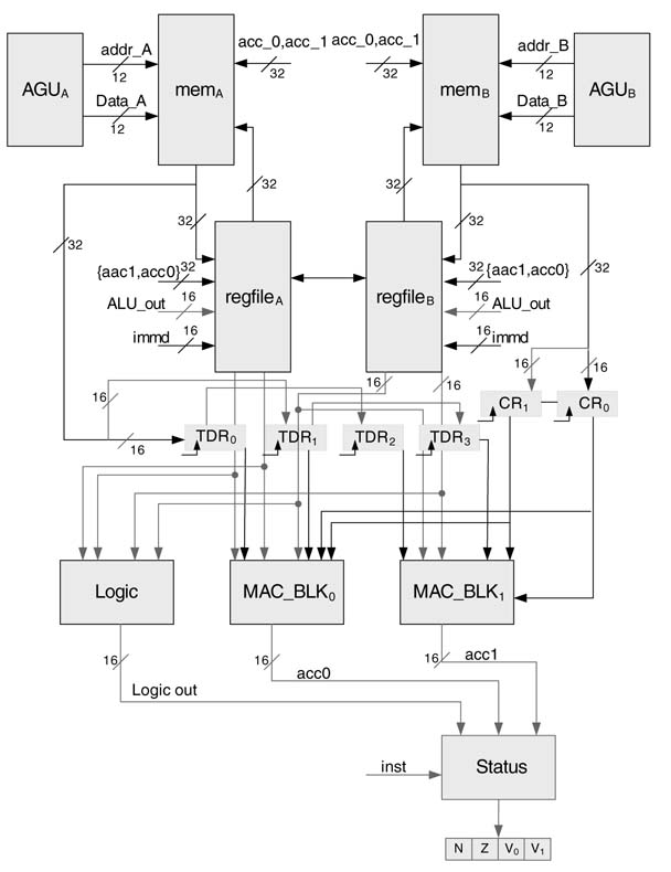
The most intensive part of the algorithm is to perform convolutionwitha512-coefficient FIR filter. The coefficients are also updated when voice activity is detected on the far-end speech signal. To perform these operations effectively, the datapath has two MAC blocks with two multipliers and one adder in each block. These blocks support application-specific instructions of filtering and adaptation of coefficients. The two adders of the MAC blocks can also be independently used as general-purpose adders or subtractors. The accelerator also supports logic instruction such as AND, OR and EXOR of two operands. The engine has two register files to store the coefficients and input data. Figure 11.8 shows the complete datapath of the accelerator.

Figure 11.8 Datapath of the multi-channel line echo canceller

Register Files

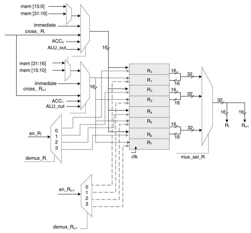
The datapath has two 16-bit register files, A and B, with 8 registers each. Each register file has one read port to read 32-bit aligned data from two adjacent registers R_i and R_i+1 (i = 0, 2, 4, 6), where R є {A, B}, or 16-bit data from memory in any of the registers in the file. The 32-bit aligned data from memory mem_R[31:0] can be written in the register files at two consecutive registers. A cross-path enables copying of the contents of two aligned registers from one register file to the other. The accelerator also supports writing a 16-bit result from ALU operations to any register, or ACC₀ and ACC1 in two consecutive registers. A 16-bit immediate value can also be written in any one of the registers. A register transfer level (RTL) design of one of the register files is given in Figure 11.9.

Figure 11.9 RTL design of one of the register files

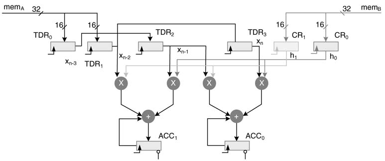
Special Registers

The datapath has two sets of special registers for application-specific instructions. Four 16-bit registers are provided to support tap-delay line operation of convolution. The data is loaded from mem_A to tap-delay line registers TDR₀ and TDR₁, while the contents of these registers are shifted to TDR₂ and TDR ₃ in the same cycle. Similarly to store the coefficients, two coefficient registers CR₀ and CR₁ are provided that are used to store the values of coefficients from mem_B. These registers are shown in Figure 11.8.

Arithmetic and Logic Operations

The accelerator can perform logic operations of AND, OR and EXOR and arithmetic operations of x, + and – on two 16-bit operands stored in any register files:

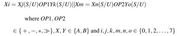
The accelerator can perform two parallel ALU operations on two sets of 16-bit operands from consecutive registers:

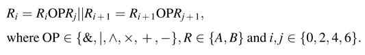
The || symbol signifies that the operations are performed in parallel.

Status Register

Two of the status register bits are used to support conditional instructions. These bits are set after the accelerator executes a single arithmetic or logic operation on two operands. These bits are Z and N for zero and negative flags, respectively. Beside these bits, two bits V₀ and V₁ for overflow are also provided for the two respective MAC blocks. One bit for each block shows whether the result of arithmetic operation in the block or its corresponding ACC_i has resulted in an overflow condition.

11.6.2.3 Address Generation Unit

The accelerator has two AGUs. Each has four registers arXi (i = 0… 3) and X є {A, B}, and each register is 12 bits wide. Each AGU is also equipped with an adder/subtractor for incrementing and decrementing addresses and adding an offset to an address. The AGU can be loaded with an immediate value as address. The AGU supports indirect addressing with pre- and post- increment and decrement. The value of the address register can also be stored back in respective memory blocks. The RTL design of the AGU for addressing memory block A is shown in Figure 11.10.

Figure 11.10 Address generation unit A

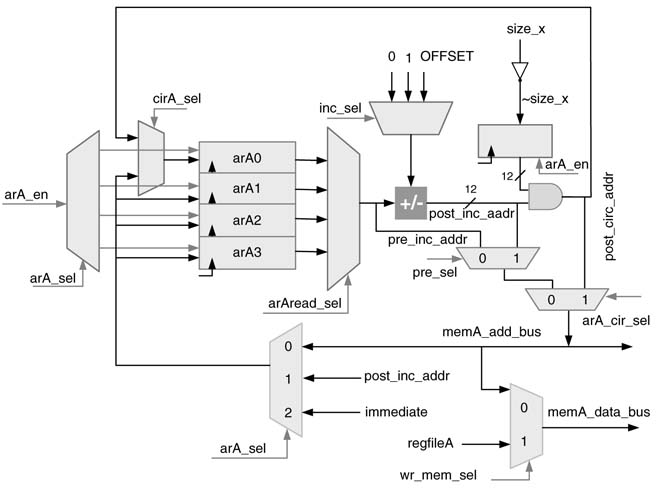
Address registers arA 0 and arB 0 can also be used for circular addressing. For circular addressing the AGU adds OFFSET to the content of the respective register, AND operation then performs modulo-by- SIZE operation and stores the value in the same register. The size of the circular buffer SIZE should always be a power of 2, and the cicular buffer must always be placed at memory address with log₂SIZE least significant zeros. The logic to perform modulo operation is given here:

This simple example illustrates the working of the logic. Let a circular buffer of size 8 start at address 0 with address bus width 6. Assume the values ar A0 = 7 and OFFSET = 3. Ten modulo addressing logic computes the next address as:

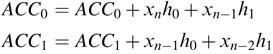
MAC Blocks

The datapath has two MAC blocks. Each MAC block has two multipliers and one adder/subtractor. The MAC performs two multiplications on 16-bit signed numbers x_n–k, h_k and x_{n–k –1}, h_{k + 1} and adds the products to a previously accumulated sum in the accumulator ACC _i:

The accumulator register is 40 bits wide. The accumulator has 8 bits as guard bits for intermediate overflows. The result in the accumulator can be rounded to 16 bits for writing it back to one of the register files. The rounding requires adding 1 to the LSB of the 16-bit value. This is accomplished by placing a 1 at the 16th bit location on accumulator reset instruction, taking the guard bits off, this bit is the LSB of the 16 bits to be saved in memory. The adder and one of the multipliers in the MAC block can also add or multiply, respectively, two 16-bit operands and store the result directly in one of the registers in the register files.

Figure 11.11 shows the configuration of the MAC blocks for maximum data reuse while performing the convolution operation. The application-specific registers are placed in a setting that allows maximum reuse of data. The taped delay line of data and two registers for the coefficients allow four parallel MAC operations for accumulating for two output samples y_n and y_n–1 as:

This effective reuse of data is shown in Figure 11.12.

Figure 11.11 Reuse of data for computing two consecutive output values of convolution summation

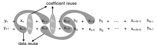
Figure 11.12 Two MAC blocks and specialized registers for maximum data reuse

11.6.2.4 Program Sequencer

The program sequencer handles four types of instruction: next instruction in the sequence, branch instruction, repeat instruction, and subroutine instruction.

11.6.2.5 Repeat Instruction

A detailed design of a loop machine is given in Chapter 10. The machine supports four nested loop instruction. The format of a loop instruction is given here.

repeat LABEL COUTN

The instructions following the loop instruction marks the start of the loop and the address of this instruction is stored in Loop Start Address (LSA) register. Address of the LABEL marks the address of the last instruction in the loop and the address is stored in Loop End Address (LEA ) register. The COUNT gives the number of times the zero overhead loop needs to be repeated and the value is stored in Loop Counter (LC) register. The logic that loop machine implements is given here

The accelerator also supports a special repeat with single instruction in the loop body. For this repeat instruction, IR and PC are disabled for any update and the instruction in the IR register is executed COUNT number of cycles before the registers are released for any updates. The format of the repeat signal instruction is given here

repeat1 COUNT

Instruction

11.6.2.6 Conditional Branch Instruction

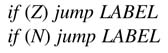
LEC accelerator supports the following jump instructions:

if (Z) jump

LABEL if (N)

jump LABEL jump LABEL

The first two conditional branch instructions check the specified status flag and if the status flag is set then the machine starts executing micro-code stored in address specified as LABEL . The design of the program sequencer for LEC accelerator is given in Figure 11.13.

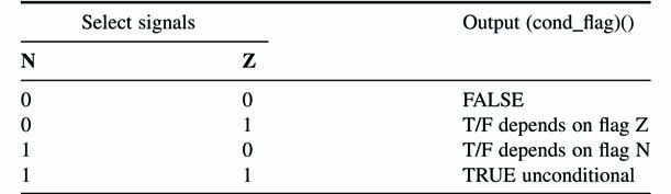
11.6.2.7 Condition Multiplexer (C_MUX)

Conditional Multiplexer logic checks if the instruction is a conditional branch instruction and accordingly set the conditional flag to the next address generation logic. The C_MUX implements the logic in Table 11.1.

11.6.2.8 Next Address Logic

The Next Address Logic (NALogic) provides the address of the next instruction to be fetched from Program Memory (PM). The block has the following inputs:

1.PC register: For normal program execution

2.Subroutine Return Address (SRA) register: This register keeps the return address of the last subroutine called and this address is used once a return to subroutine is made.

3.LSA register: This register has the loop start address of the current loop and the address is used once the loop count is not zero and the program executes the last instruction in the loop.

4.Branch Address Fields from IR: For branch instruction and subroutine calls the IR has address of the next instruction. This address is used for instructions that execute a jump or subroutine call.

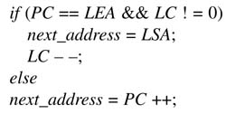
The next address block implements the following logic

if (branch || call subroutine)

next_address = IR[branch address fields]

else if (instruction == return)

next_address = SRA

else if (PC == LEA && LC ! = 0)

next_address = LSA

else

next_address = PC;

11.6.2.9 Data Memories

The accelerator has two memories each consisting N kB. For defining rest of the memory related fields in the current design, assume 8 kB of SRAM with 32-bit data bus. This makes 2048 memory locations and 11-bit address is required to access any memory location. These fields accordingly change with different memory sizes. The memories are dual-ported to give access to the DMA for simultaneous read and write in the memories.

Figure 11.13 Program sequences of the LEC accelerator

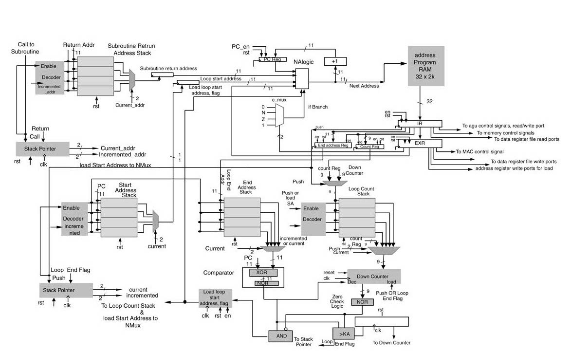
Table 11.1 Logic implemented by C_MUX (see text)

11.6.2.10 Instruction Set Design

The instruction set has some application-specific instructions for implementing LMS adaptive algorithm. These instructions perform 4 MAC operations utilizing the tap-delay line registers and coefficients registers. Beside these instructions, the accelerator supports many general-purpose instructions as well.

The accumulator supports load and store instructions in various configurations.

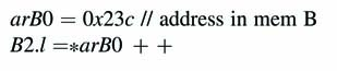
11.6.2.11 Single Load Long Instruction

The instruction loads a 32 bit word stored at address location pointed by ar Xj register and the instruction also post increment or decrement the address as defined in the instruction. The terms in the brackets show the additional options in any basic instruction.

Example:

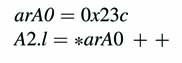
This instruction stores the 32-bit content at memory location 0x23c in A2, A3 registers. Similarly the same instructions for B register file are given here:

11.6.2.12 Parallel Load Long Instructions

The two load instruction on respective register files A and B can be used in parallel as well. The format of the instruction is given here:

where i , m є {0,2,4} and j , n є {0,1,2,3}

11.6.2.13 Single and Parallel Load Short Instruction

This instruction loads a 16 bit value pointed by ar Xj in Xi register. The address register can optionally be post incremented or decremented.

Two of these instructions on respective register files A and B can be used in parallel as well. The instruction format is shown here

These instructions are orthogonal and can be used as mix of short and long load instructions in parallel.

11.6.2.14 Single Long Store Instruction

11.6.2.15 Parallel Long Store Instruction

11.6.2.16 Single and Parallel Load Short Instruction

11.6.2.17 Pre-increment Decrement Instruction

All the load and store instruction support pre increment/decrement addressing as well. In this case the address is first incremented or decremented as defined and then used for memory access. For example the single load instruction with pre-increment addressing is coded as

11.6.3 Address Registers Arithmetic

Load Immediate Address in an Address Register. . . .

This instruction loads an immediate value CONST as address into any one of the registers of an address register file.

A 12-bit constant offset OFFSET can be added or subtracted in any register of the address register files and the result can be stored in the same or any other register in the register files.

Example:

The instruction adds 0x131 in the content of arB2 and stores the value back in arA0 address register.

11.6.3.1 Circular Addressing

The accelerator supports circular addressing where the size of the circular buffer N should be a power of 2 and needs to be placed in memory address with log₂N least significant zeroes in the address.

11.6.3.2 Arithmetic and Logic Instruction

The accelerator supports one logic and two arithmetic instructions on 16-bit signed or unsigned (S/U) operands. The instruction format is

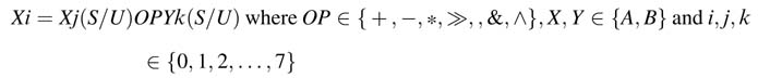
The shift is performed using the multiplier in the MAC block. Two of the arithmetic instructions can be used in parallel, the destination registers of the two parallel instructions should be in different register files.

The conditional flags of N and Z are only set if the accelerator executes a single arithmetic and logic instruction.

11.6.3.3 Accumulator Instructions

The value of accumulator is truncated and 16 bits (31:16) of the respective Acc are stored in any register of the register files. In case of single instruction execution the condition flags are also set.

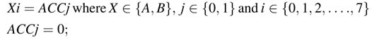
This instruction resets the ACC regsiter.

This instruction resets the register and places one at 15^th bit location for rounding.

This instruction performs MAC operation, where F and I are used to specify fraction or integer mode of operations.

This instruction multiplies two signed or unsigned operands in fraction or integer mode and store them in the ACC.

Two of these instructions can be used in parallel for both the ACC registgers. For example the instruction here implements two MAC operations on signed operands in parallel.

11.6.3.4 Branch Instruction

The accelerator supports conditional and unconditional branch instructions. Two flags that are set as a result of single arithmetic instructions are used to make the decision. The instructions are

The accelerator also supports unconditional instruction

Where LABEL is the address of the next instruction the accelerator executes if the condition is true, otherwise the accelerator keeps executing instructions in a sequence.

11.6.3.5 Application Specific Instructions

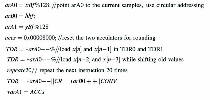
The accelerator supports application specific instructions for accelerating the performance of convolution in adaptive filtering algorithms. In signal processing the memory accesses are the main bottlenecks of processing data. Inherently in many signal processing algorithms especially while implementing convolution summation the data is reused across multiple instructions. This reuse of data is exploited by providing a tap delay line and registers for filter coefficients. The data can be loaded in tap delay line registers TDR0 and TDR1 and coefficient registers CR0 and CR1 for optimal filtering operation:

The instruction saves the 32-bit of data from the address pointed by arA 0 in Tap Delay Line by storing the two 16-bit samples in TDR0 and TDR1 while respectively shifting the older values into TDR2 and TDR3. The instruction also decrements the address stored in the address register for accessing the new samples in the next iteration. Similarly, the coefficients stored at address pointed by arB1 are also read in coefficient registers CR0 and CR1 while the address register is incremented by 1. The datapath in the same cycle performs four MAC operations:

The 16-bit values in two accumulators ACC0 and ACC1 are stored in memory location pointed by ar X register.

Example: The MAC units along with special registers are configured for adaptive filter specific instructions. The MAC units can perform four MAC operations to simultaneously compute two output samples.

The values of x_n and x _{n – 1} are loaded first in the TDL and subsequently x_{n – 2} and x_{n – 3} are loaded in the TDL while h₀ and h₁ are loaded in CRs. The length of the filter is 40. The convolution operation is performed in a loop N/2 number of times to compute the two samples, use circular addressing.

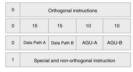
11.6.3.6 Instruction Encoding

Though the instruction can be encoded in a way that saves complex decoding but in this design a simple coding technique is used to avoid complexity. The accelerator supports both regular and special instructions (Figure 11.14.) The regular instructions are a set of orthogonal instructions that are identical for both the data paths and AGUs.A0atbit location0identifies that the sub-instructions in the current instruction packet are orthogonal and a 1 at the bit location specifies that this is a special or non orthogonal instruction.

Figure 11.14 Instruction encoding

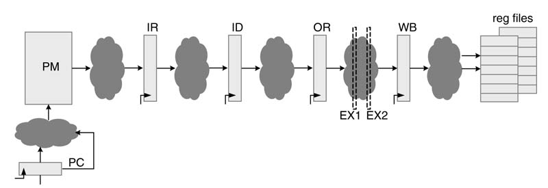
11.6.4 Pipelining Options

The pipelining in the datapath is not shown but the accelerator can be easily pipelined. Handling pipeline hazard is an involved area and good coverage of pipelining hazards can be found in [21]. An up to six pipeline stages are suggested. In the first stage an instruction is fetched from PM into an Instruction Register. The second stage of pipeline decodes the instruction and in third stage operands are fetched in the operand registers. A host of other operations related to memory reads and writes and address-register arithmetic can also be performed in this cycle. The third stage of pipelining performs the operation. This stage can be further divided to use pipelined multipliers and adders. The last stage of pipelining writes the result back to the register files. Figure 11.15 proposes a pipelined design of the accelerator. The pipeline stages are Instruction Read (IR), Instruction Decode (ID), Operand Read (OR), and optional pipelining in execution unit as Execution 1 (EX1) and Execution 2 (EX2), and finally Write Back (WB) stage.

11.6.4.1 Delay Slot

Depending upon the number of pipeline stages, the delay slot can be effectively used to avoid pipeline stalls. Once the program sequencer is decoding a branch instruction the next instruction in the program is fetched. The program can fill the delay slot with a valid instruction that logically precedes the branch instruction but is placed after the instruction. The delay slot instruction must not be a branch instruction. In case the programmer could not effectively use the delay slot, it should be filled with NOP instruction.

Figure 11.15 Pipeline stages for the LEC accelerator

11.6.5 Optional Support for Coefficient Update

In the design of micro-coded state machine, HW support can also be added to speedup coefficients update operation of (11-3). This requires addition of a special error register ER that saves the scaled error value µe[n] and few provisions in the datapath for effective use of multipliers, adders and memory for coefficient updates. This additional configuration is given in Figure 11.16. This augmentation in the datapath and AGUs can be simply incorporated in the existing design of the respective units given in Figure 11.8 and Figure 11.10 with additional address register in the AGU, interconnections and multiplexers. The setting assumes arB0 stores the address of the coefficient buffer. The coefficient memory is a dual port memory that allows reading and writing of 32-bit word simultaneously. The current value of the address in arB0 register is latched in the delay address register arB0D for use in the subsequent write in mem_B. The updated coefficients are calculated in ACCs and are stored in the coefficient buffer in the next cycle.

arB0 =hBf

arA0 = xBf %256

ER = A0*B0; // assuming μin A0 and e[n] is in B0 registers

CR = *arB0++ || TDR=*arA0--%

repeat1 20

CR=*arB0++||TDR=*arA0--||UPDATE

Figure 11.16 Optional additional support for coefficient updating

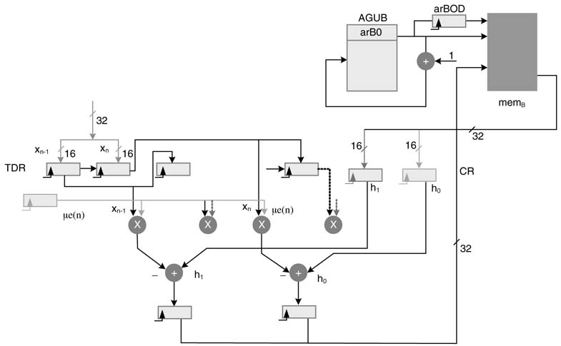
The UPDATE micro-code performs the following operations in HW in a single cycle:

ACC0 = CR0-TR0*ER
ACC1 = CR1 – TR1*ER
*arB0D = truncate{ACC1,ACC0}

This setting enables the datapath to update two coefficients in one cycle. The same cycle loads values of two new input samples and two coefficients.

11.6.6 Multi MAC Block Design Option

The datapath can be easily extended to include more MAC blocks to accelerate the execution of filtering operation. A configuration of the accelerator with four MAC blocks is depicted in Figure 11.17.

It is important to highlight that the current design can easily be extended with more number of MAC blocks for enhanced performance. The new design still works with just loading two samples of data and two coefficients of the filter from the two memories respectively.

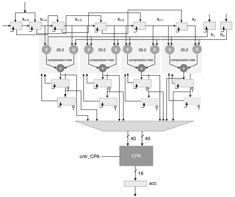
11.6.7 Compression Tree and Single CPA-based Design

The design can be further optimized for area by using compression trees with a single CPA. The design is shown in Figure 11.18. Each MAC block is implemented with a single compression tree where the partial sum and partial carry are saved in a set of two accumulator registers. These registers also form two partial products in the compression tree. At the end of the convolution calculation, these partial sums and carries are added one by one using the CPA.

Figure 11.17 Optional additional MAC blocks for accelerating convolution calculation

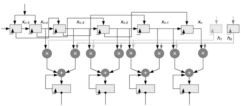
Figure 11.18 Optional use of compression trees and one CPA for optimized hardware

Exercises

Exercise 11.1

Add bit-reverse addressing support in the arA0 register of the AGU. The support increments and decrements addresses in bit-reverse addressing mode. Draw RTL diagram of the design.

Exercise 11.2

Add additional TDL registers and MAC blocks in Figure 11.12 to support IIR filtering operation in adaptive mode.

Exercise 11.3

Add additional hardware support with an associated MAC to compute x _n x^T_n while performing a filtering operation. Use this value to implement the NLMS algorithm of (11.4.)

Exercise 11.4

Using the instruction set of the processor, write code to perform division using the Newton Repson method.

References

1. S. Haykin, Adaptive Filter Theory, 4th edn, 2002, Prentice-Hall.

2. B. Farhang-Boroujeny, Adaptive Filters: Theory and Applications, 1998, Wiley.

3. S. F. Boll and D. C. Pulsipher, “Suppression of acoustic noise in speech using two-microphone adaptive noise cancellation ,” IEEE Transactions on Acoustic Speech, SignaI Processing, 1980, vol. 28, pp. 752–753.

4. Kuo, S. M. Huang and Y. C. Zhibing Pan, “Acoustic noise and echo-cancellation microphone system for video conferencing,” IEEE Transactions on Consumer Electronics, 1995, vol. 41, pp. 1150–1158.

5. R. H. Kwong and E. W. Johnston, “Avariable step size LMS algorithm,” IEEE Transactions on Signal Processing , 1992, vol. 40, pp. 1633–1642.

6. J.-K. Hwang and Y.-P. Li, “Variable step-size LMS algorithm with a gradient-based weighted average , ” IEEE Signal Processing Letters , 2009, vol. 16, pp. 1043–1046.

7. G. A. Clark, S. K. Mitra and S. R. Parker, “Block implementation of adaptive digital filters ,” IEEE Transactions on Circuits and Systems, 1981, vol. 28, pp. 584–592.

8. S. Sampei, “Rayleigh fading compensation method for 16QAM modem in digital land mobile radio systems , ” IEICE Transactions on Communications, 1989, vol. 73, pp. 7–15.

9. J. K. Cavers, “An analysis of pilot symbol assisted modulation for Rayleigh fading channels,” IEEE Transactions on Vehicular Technology, 1991, vol. 40, pp. 686–693.

10. S. Sampei and T. Sunaga, “Rayleigh fading compensation for QAM in land mobile radio communications,” IEEE Transactions on Vehicular Technology, 1993, vol. 42, pp. 137–147.

11. H.-B. Li, Y. Iwanami andT. Ikeda, “Symbol error rate analysis for MPSK under Rician fading channels with fading compensation basedontime correlation , ” IEEE Transactionson Vehicular Technology, 1995, vol. 44, pp. 535–542.

12. T. M. Schmidl and D. C. Cox, “Robust frequency and timing synchronization for OFDM,” IEEE Transactions on Communications, 1997, vol. 45, pp. 1613–1621.

13. J. P. Costa, A. Lagrange and A. Arliaud, “Acoustic echo cancellation using nonlinear cascade filters,” in Proceedings of IEEE International Conference on Acoustics, Speech and Signal Processing, 2003, vol. 5, p. V–389–392.

14. Stenger and W. Kellermann, “Nonlinear acoustic echo cancellation with fast converging memoryless preprocessor,” in Proceedings of IEEE International Conference on Acoustics, Speech an Signal Processing, 2000, vol. 2, pp. II-805–808.

15. Guerin, G. Faucon and R. L.Bouquin-Jeannes, “Nonlinear acoustic echo cancellation based on Volterra filters,” IEEE Transactions on Speech Audio Processing, 2003, vol. 11, pp. 672–683.

16. V. Krishna, J. Rayala and B. Slade, “Algorithmic and implementation aspects of echo cancellation in packet voice networks,” in Proceedings of 36th IEEE Asilomar Conference on Signals, Systems and Computers, 2000, vol. 2, pp. 1252–1257.

17. International Telecommunications Union, (ITU). G.168: “Digital network echo cancellers,” 2004.

18. H. Ye and B. X. Wu, “A new double-talk detection based on the orthogonality theorem,” IEEE Transactions on Communications, 1991, vol. 39, pp. 1542–1545.

19. T. Gansler, M. Hansson, C.-J. Ivarsson and G. Salomonsson, “A double-talk detector based on coherence,” IEEE Transactions on Communications, 1996, vol. 44, pp. 1421–1427.

20. J. Benesty, D. R. Morgan and J. H. Cho, “A new class of doubletalk detectors based on cross-correlation,” IEEE Transactions on Speech and Audio Processing, 2000, vol. 8, pp. 168–172.

21. J. L. Hennessy and D. A. Patterson, Computer Architecture: a Quantitative Approach, 4th edn, 2007, Morgan Kaufmann Publishers, Elsevier Science, USA.

22. D. G. Manolakis, V. K. Ingle and S. M. Kogon, Statistical and Adaptive Signal Processing, 2000, McGraw-Hill.

23. S. G. Sankaran and A. A. Beex, “Convergence behavior of affine projection algorithm,” IEEE Transactions on Signal Processing, 2000, vol. 48, pp. 1086–1096.