
6
Reproducing Kernel Hilbert Space Models for Signal Processing
6.1 Introduction
In this chapter we introduce a set of signal models properly defined in an RKHS. The set of processing algorithms presented here are collectively termed an RSM because they share a distinct feature; namely, all of them intrinsically implement a particular signal model (like those previously described in Chapter 2) whose equations are written in the RKHS generated with kernels. For doing that, we exploit the well‐known kernel trick (Schölkopf and Smola, 2002), and this is the most usual approach to kernel‐based signal processing problems in the literature. Quite often one is interested in describing the signal characteristics by using a specific signal model whose performance is hampered by the (commonly strong) assumption of linearity. As we already know, the use of the theory of reproducing kernels can circumvent this problem by defining nonlinear algorithms by simply replacing dot products in the feature space by an appropriate Mercer kernel function (Figure 6.1). The most famous example of this kind of approaches is the support vector classification (SVC) algorithm, which has yielded a vast number of applications in the field of signal processing, from speech recognition to image classification.

Figure 6.1 In SVM estimation problems, a nonlinear relationship between data points in the input space is transformed into a linear relationship between mapped data into the (higher dimensional) RKHS. Different signal model equations can be used in the RKHS, as far as the problem statement is expressed in terms of dot products.
We should note first that nonlinear SVM for DSP algorithms can be obtained from nonlinear versions of linear algorithms presented in Chapter 5. However, nonlinear SVM for DSP algorithms can be developed from two different general approaches, which are presented in this chapter and in Chapter 7. In this chapter, we will focus on a class of SVM for DSP algorithms that consists of stating the signal model of the time‐series structure in the RKHS, and hence they are called RSM algorithms. Several examples of SVM‐DSP in this setting are nonlinear system identification and antenna array processing. These and some other examples are summarized in this chapter, both in terms of theoretical foundations and of practical applications.
In particular, the chapter pays attention to the fundamental elements of the RSM approach. We concentrate on particular signal structures which have been previously studied. After their definition, nonlinear versions of the signal models will be developed. Specifically, the chapter is devoted to the study of:
- nonlinear ARX system identification techniques;
- nonlinear FIR and γ‐filter structures;
- array processing, both with temporal and spatial reference;
- semiparametric regression (SR).
Examples are used to consolidate the main concepts (nonlinear system identification), and application examples are further provided (electric network modeling and array structures from communication systems).
6.2 Reproducing Kernel Hilbert Space Signal Models
The background for stating signal models in the RKHS is well established, and it has been widely used in the kernel literature. In this section, we limit ourselves to stating a general signal model for estimation with discrete‐time series notation, which will be useful for immediately summarizing the relevant elements of three SVM for DSP algorithms in this setting, following the framework in Rojo‐Álvarez et al. (2014). On the one hand, nonlinear ARX system identification and γ‐filter system identification use a signal model equation in the RKHS relating an exogenous time series and an observed data time‐series. On the other hand, antenna array processing with spatial reference uses an energy expression in the RKHS, together with complex‐valued algebra.
The proof is straightforward (and similar to the demonstration for deriving the PSM), by using the conventional Lagrangian functional and dual problem. This is the mostly used approach to tackle nonlinear problems with kernels in general and to tackle signal processing problems with SVM in particular. This theorem is next used to obtain the nonlinear equations for several DSP problems. Before doing that, we summarize two relevant properties that will be useful for further developments.
A concept that has been largely used in RKHS in SVM for DSP is the composite kernel, which will give flexibility for defining relationships between two observed signals (exogenous and system output), by means of an RKHS system identification model.
Note that this measure of similarity between different data observations is different to the traditional stacked approach in the input space. The common approach when dealing with different data entities, variables, or observations, here c and d, is to concatenate them in the input space and then to define a mapping function ϕ and its corresponding kernel function to work with them. This approach has been widely used in time series analysis, as we will see in Section 6.2.1. By doing so, however, one loses the signal model structure.
An important second difference is that stacking vectors in feature spaces leads to considering dedicated kernels to each variable separately, whose similarity functions are then summed up. The model is limited in the sense that variable cross‐relations are not considered. The summation kernel expression can be readily modified to account for the cross‐information among the different variables, in our case between an exogenous and an output observed data time series.
If the dot product is computed, we obtain

where ![]() ,
, ![]() , and
, and ![]() are three independent definite‐positive matrices.Note that c and d must have the same dimension for the formulation to be valid, otherwise K3 cannot be computed.
are three independent definite‐positive matrices.Note that c and d must have the same dimension for the formulation to be valid, otherwise K3 cannot be computed.
6.2.1 Kernel Autoregressive Exogenous Identification
As we have seen in the introductory chapters, a common problem in DSP is to model a functional relationship between two simultaneously recorded discrete‐time processes (Ljung, 1999). When this relationship is linear and time invariant it can be addressed by using an ARMA difference equation, and when a simultaneously observed set of signal samples {xn} is available, called an exogenous signal, the parametric model is called an ARX signal model for system identification.
Many approaches have been considered to tackle this important problem of ARX system identification. General nonlinear models, such as artificial neural networks, wavelets, and fuzzy models, are common and effective choices (Ljung, 1999 ; Nelles, 2000), though their temporal structure cannot be easily analyzed, because it remains inside a black‐box model. In the last decade, enormous interest has been paid to kernel methods in general and SVM in particular in this setting. The first approaches considered the SVM version for regression, the so‐called SVR method. In particular, Drezet and Harrison (1998), Goethals et al. (2005b), and Espinoza et al. (2005) used the SVR algorithm for nonlinear system identification. However, in all these studies the time series structure of the data was not scrutinized and the approach essentially consisted of stacking the signals that were then fed to the SVR. Alternatively, Rojo‐Álvarez et al. (2004) explicitly formulated SVM for modeling linear time‐invariant ARMA systems (linear SVM‐ARMA), and this kind of formulation has been recently extended to a general framework for linear signal processing problems (Rojo‐Álvarez et al., 2005). However, if linearity cannot be assumed, then nonlinear system identification techniques are required.
We next summarize several SVM for DSP procedures for nonlinear system identification. The material has been presented in detail by Martínez‐Ramón et al. (2006), Camps‐Valls et al. (2009b), and Camps‐Valls et al. (2007a), so we summarize the most relevant details here. First, the stacked SVR algorithm for nonlinear system identification is briefly examined in order to check that, though efficient, this approach does not correspond explicitly to an ARX model in the RKHS.
Let {xn} and {yn} be two discrete‐time signals, which are the input and the output respectively of a nonlinear system. Let yn = [yn−1, yn−2, …, yn−M]T and xn = [xn, xn−1, …, xn−Q+1]T denote the states of input and output at time instant n. The stacked‐kernel system identification algorithm (Gretton et al., 2001a ; Suykens et al., 2001a) can be described as follows.
Note that this is the expression for a general nonlinear system identification, but it does not correspond to an ARX structure in the RKHS. Moreover, though the reported performance of the algorithm is high when compared with other approaches, this formulation does not allow us to scrutinize the statistical properties of the time series that are being modeled in terms of autocorrelation and/or cross‐correlation between the input and the output time series.
Composite kernels can be introduced at this point, allowing us to next introduce a nonlinear version of the linear SVM‐ARX algorithm by using actually an ARX scheme on the RSM. After noting that the cross‐information between the input and the output is lost with the stacked‐kernel signal model, the use of composite kernels is proposed for taking into account this information and for improving the model versatility.
Two different kernel functions can be further identified:
which account for the sample estimators of input and output time‐series autocorrelation functions (Papoulis, 1991) respectively in the RKHS. Specifically, they are proportional to the non‐Toeplitz estimator of each time series autocorrelation matrix.
The dual problem consists of maximizing the PSM dual problem (see Equation 5.7) with Rs = Rx + Ry, and the output for a new observation vector is obtained as

The kernels in the preceding equation correspond to correlation matrices computed into the direct summation of kernel spaces ![]() 1 and
1 and ![]() 2. Hence, the autocorrelation matrices’ components given by xn and yn are expressed in their corresponding RKHS and the cross‐correlation component is computed in the direct summation space. A third space can be used to compute the cross‐correlation component, which introduces generality to the model.
2. Hence, the autocorrelation matrices’ components given by xn and yn are expressed in their corresponding RKHS and the cross‐correlation component is computed in the direct summation space. A third space can be used to compute the cross‐correlation component, which introduces generality to the model.
Note that, in this case, xn and yn need to have the same dimension, which can be naively accomplished by zero completion of the embeddings.
Therefore, despite the fact that SVM‐ARX and SVR nonlinear system identifications are different problem statements, both models can be easily combined.
6.2.2 Kernel Finite Impulse Response and the γ‐filter
As described in previous chapters, many NN structures with a linear memory stage followed by a non‐linear memoryless stage are commonly used in signal processing, such as the time delay NN and the focused γ‐network. These networks offer good performance at the expense of increasing the dimensionality of the state vector of the linear memory stage, and thus training the memoryless stage involves both high computational burden and risk of overfitting. In Camps‐Valls et al. (2009b), a set of kernel methods are introduced in order to develop nonlinear γ‐filters in a straightforward yet principled way. These RKHS algorithms for nonlinear system identification with γ‐filters are summarized next.
This property can be readily used to derive the nonlinear γ‐filters with composite kernels and with tensor‐product kernels, as detailed and benchmarked in Camps‐Valls et al. (2009b).
6.2.3 Kernel Array Processing with Spatial Reference
An antenna array is a group of (usually identical) electromagnetic radiator elements placed in different positions of the space. This way, an electromagnetic flat wave illuminating the array produces currents that have different amplitudes and phases depending on the DOA of the wave and of the position of each radiating element. The discrete‐time signals collected from the array elements can be seen as a time and space discrete process.
The fundamental property of the array is that it is able to detect the DOA of one or several incoming signals or it is able to discriminate one among various incoming signals provided they have different DOAs (Van Trees, 2002). Applications of antenna array processing range from radar systems (which minimize the mechanical components by electronic positioning of the array radiation beam), to communication systems (in which the system capacity is increased by the use of spatial diversity), and to radioastronomy imaging systems, among many others.
The array processing problem stated in Equation 3.51 can be solved when there are no training symbols available, but just a set of incoming data and information about the angle of arrival of the desired user. In this case, the algorithm to be applied consists of a processor that detects without distortion (distortionless property) the signal from the desired DOA while minimizing the total output energy. The signal can be easily mapped to an RKHS, and the algorithm must optimize
for a given set of previously collected snapshots, and Φ is a matrix containing all mapped snapshots ϕ(xn).
These kernels cannot be directly used because an expression for R is not available in an infinite‐dimension RKHS. A kernel eigenanalysis introduced by Schölkopf et al. (1998) leads to the kernel expression
where Φ is a matrix containing all the incoming data used to compute the autocorrelation matrix R, and K0 is a kernel matrix containing all dot products ![]() . These kernels can be used to solve a dual problem equal to the one of Property 24. The primal coefficients can be expressed as
. These kernels can be used to solve a dual problem equal to the one of Property 24. The primal coefficients can be expressed as
where ![]() are complex‐valued dual coefficients.
are complex‐valued dual coefficients.
6.2.4 Kernel Semiparametric Regression
SR has been a widely studied topic in conventional statistics. It supports the idea that some phenomena under analysis can be represented with parametric models, especially using linear regression, and by nonparametric models, when the explicit relationship between the input and the output turns to be more complicated to know. Given that the knowledge path can be thought of as usually going from nonparametric to parametric models, SR combines both approaches. The most widely known method for SR is the Nadayara–Watson (NW) estimator. In this section, we start defining the fundamentals of this classical estimator, and then we show how it can be readily expressed in terms of a composite kernel in the RSM framework.
In addition, we introduce in this chapter the use of bootstrap resampling techniques (BRTs) in SVM for RSM models. We focus on the role that it has played for model diagnosis and for analyzing the statistics of the model parameters, specially for SR. This section paves the way toward the use of these popular nonparametric methods for working with confidence intervals and for establishing statistical tests in this setting.
Nadayara–Watson Estimator for Semiparametric Regression
Let yi be the ith observation of a response variable and ![]() be the K‐dimensional ith vector containing the observed predictor variables (i = 1, …, N), where T denotes the transposed vector. The constant unit level is introduced to take into account the interception component.
be the K‐dimensional ith vector containing the observed predictor variables (i = 1, …, N), where T denotes the transposed vector. The constant unit level is introduced to take into account the interception component.
The simplest parametric regression model is the general linear model:
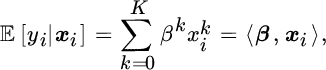
where ![]() denotes conditional statistical expectation, and 〈⋅, ⋅〉 is the dot product. Model coefficients β1, …, βK, and interception β0, are estimated by ordinary LS.
denotes conditional statistical expectation, and 〈⋅, ⋅〉 is the dot product. Model coefficients β1, …, βK, and interception β0, are estimated by ordinary LS.
Nonparametric kernel regression (Ruppert et al., 2003) computes a local weighted average of the criterion variable given the values of the predictors; that is:
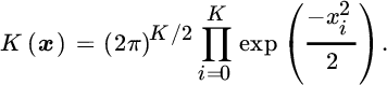
where m(⋅) is a nonparametric function. For instance, the NW estimator consists of a constant‐kernel approximation given by

with

and
Parameter σ is called the bandwidth, and it represents the neighborhood of influence for each observation. A smaller bandwidth will give a lower bias but increased variance in the estimator, whereas a larger bandwidth will produce higher bias (model mismatch) despite a reduced variance estimator.
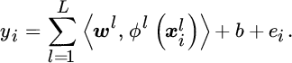
The SR model can be very useful when mixed nature predictor variables are available (for instance, metric and dichotomic), because different components can be modeling the contribution of each subset of variables. Also, sometimes we have some a priori knowledge about the model that we can assume for a subset of variables, but the remaining subset has a completely unknown nature. Without loss of generality, let us assume observation vectors that are composed of D dichotomic variables and M metric variables, ![]() . Let us use a parametric, linear component for the dichotomic variables, and a nonparametric, nonlinear component for the metric variables. The corresponding SR model is
. Let us use a parametric, linear component for the dichotomic variables, and a nonparametric, nonlinear component for the metric variables. The corresponding SR model is
The estimation method is described in Heerde et al. (2001) and Lee and Nelder (1996), and it is briefly presented here. The model can be written down as
where ei denotes the ith residual. By taking the conditional average with respect to the parametric variables, we obtain
Then, by subtracting Equations 6.33 and 6.34, we have
Therefore, a three‐step procedure can be stated. First, averages conditional to the nonparametric variables are estimated for the response variable and for the parametric variables, given by


Note that bandwidths σ1 and σ2 must be properly chosen for the statistical estimation. Second, the new response variable ![]() and the new predictor variables
and the new predictor variables ![]() are used to find
are used to find ![]() by solving
by solving
by means of ordinary LS. Note that the intercept term disappears at this step because of the mean subtraction, so that it remains inside the nonparametric component. Third, the nonparametric component is obtained by nonparametric regression on ỹ; that is:

where bandwidth σ3 must be also properly fixed. The choice of three different bandwidths must be addressed, with two of them coming from a nonparametric estimation of the pdf and the third one coming from the nonparametric regression process. Several bandwidth selection techniques are available, among which are Lee’s rule of thumb, cross‐validation, or subjective approach (Heerde et al. 2001 ; Lee and Nelder 1996).
Some limitations of the procedure could be present according to this formulation:
- Automatic selection procedures can deteriorate when low‐sized data sets are analyzed.
- The denominators in Equations 6.36, 6.37, and 6.39 can become very small for a newly tested point that is far enough from the observations, and this produces an unbounded predicted output. Again, this situation can be more present when reduced data sets are under analysis. A solution for this drawback can be the introduction of a small threshold parameter in the exponential exponent, which is, in fact, a regularization procedure. This threshold should be also found as a free parameter.
- Finally, all the available observations are used for building the solution in Equation 6.39, independently of their adequacy or noise level. This solution will not be operational for studies with high number of observations.
These limitations can be alleviated by the SVM formulation for SR, which is presented next.
Semiparametric Regression Approach using the Support Vector Machine
An alternative formulation of SR can be stated by using the RSM framework. Let us assume that the model can be expressed with two additive contributions: one from the parametric and another from the nonparametric predictor variables. Let us assume also that there exists a possibly nonlinear transformation of the metric predictor variables into a higher (possibly infinite) dimensionality space, ![]() , where ℱm is known as the feature space for the metric model component. The main property of this nonlinear transformation is that a linear regression operator can be found in the feature space, given by vector
, where ℱm is known as the feature space for the metric model component. The main property of this nonlinear transformation is that a linear regression operator can be found in the feature space, given by vector ![]() . Let us finally assume that, for the dichotomic model component, there exists another transformation of the dichotomic vectors
. Let us finally assume that, for the dichotomic model component, there exists another transformation of the dichotomic vectors ![]() to a different feature space
to a different feature space ![]() d where another linear regression operator
d where another linear regression operator ![]() can be properly adjusted.
can be properly adjusted.
In these conditions, the joint regression model is given by
Here, the reference interception term br can be previously fixed, in order to make easy the comparison to a given level. For instance, br could be the average sales level constrained to nonpromotional periods, so that the resulting model will provide us with information about the predictors either increasing or decreasing that level.
The SVM‐SR algorithm is stated as the minimization of the ɛ‐Huber cost plus a regularization term given by the ℓ2 norm of the weights in the feature spaces; that is:

constrained to
where ξi and ![]() (in the following, denoted jointly by
(in the following, denoted jointly by ![]() ) are the slack variables used to account for the residuals in the model; I1 is the set of samples for which
) are the slack variables used to account for the residuals in the model; I1 is the set of samples for which ![]() , and I2 is the set of samples for which
, and I2 is the set of samples for which ![]() . Following the usual SVM formulation methodology, Lagrangian functional ℒ can be written down, and by making zero its gradient with respect to the primal variables we obtain
. Following the usual SVM formulation methodology, Lagrangian functional ℒ can be written down, and by making zero its gradient with respect to the primal variables we obtain


with αi and ![]() denoting the Lagrange multipliers that correspond to Equation 6.45 and Equation 6.46 respectively. Matrix notation is introduced as follows:
denoting the Lagrange multipliers that correspond to Equation 6.45 and Equation 6.46 respectively. Matrix notation is introduced as follows:
Finally, the dual problem can be stated (Rojo‐Álvarez et al., 2004) as the maximization of

constrained to Equation 6.47, with respect to dual variables ![]() . After this quadratic programming problem is solved, and according to Equations 7.29, 6.45, and 6.46, the final expression of the solution can be easily shown to be given by the following expression:
. After this quadratic programming problem is solved, and according to Equations 7.29, 6.45, and 6.46, the final expression of the solution can be easily shown to be given by the following expression:

where ![]() . Note that the estimated response variable ŷ is calculated from a weighted expansion of dot products in the feature spaces. With this expression for the solution, the explicit calculation of wm and vd is not required.
. Note that the estimated response variable ŷ is calculated from a weighted expansion of dot products in the feature spaces. With this expression for the solution, the explicit calculation of wm and vd is not required.
Here, we are mainly concerned about two properties of Mercer kernels: (1) the sum of two Mercer kernels is a Mercer kernel; and (2) the product of a Mercer kernel times a positive constant is a Mercer kernel. These simple properties allows us to propose the use of a scaled linear kernel that generates the parametric component:
with ![]() , plus a nonlinear kernel that generates the nonparametric component:
, plus a nonlinear kernel that generates the nonparametric component:
Constant δ can be chosen for giving a balance between the parametric and nonparametric components. Thus, the final solution of SVM‐SR can be readily expressed as
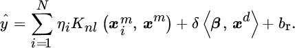
Taking Equations 6.53 and 6.56 into account, coefficients ηi determine completely both the parametric and the nonparametric components.
Bootstrap Resampling for Model Diagnosis
One of the main limitations of current SR methods is the difficulty in establishing clear cut‐off tests for the nonparametric variables of the model, and much effort is being done in this framework (Ruppert et al., 2003). Also, this aspect has not yet been completely solved in the SVM literature, and systematic procedures for establishing feature selection, significance levels, and confidence intervals (CIs) for model diagnosis have been developed (Lal et al., 2004). An interesting approach to the model diagnosis and feature selection issues in SVM for SR can be given by BRTs, which were first proposed as possibly nonparametric procedures for estimating the pdf of an estimator from a limited, but informative enough, set of observations (Efron and Tibshirani, 1998). BRTs have been successfully used before for fixing the free parameters of SVM classifiers (Rojo‐Álvarez et al., 2002) and as a feature selection strategy using the robust SVM linear maximum margin classifier (Soguero‐Ruiz et al., 2014a,b). We propose here to extend their use to model diagnosis and free parameter selection for SVM problems with the SR algorithm.
For a given set of N observations v, the dependence between the predictor variables and the response variable can be fully described by using their joint distribution:
In order to obtain the SVM‐SR model, Equation 7.33 is maximized. This estimation process is denoted by operator s(⋅), and it depends on observations v, and on the free parameters of the model that have been fixed a priori. Those free parameters can be grouped in a vector θ, that consists of the ε‐Huber cost parameters and of the kernel‐related parameters; that is, for the Gaussian kernel, θ = {ε, C, γ, δ, σ}. The SVM‐SR Lagrange multipliers obtained by using the observations and a given a priori fixed θ are
The model performance can be measured with the empirical risk, which can be defined as a merit figure of the model that is evaluated at the observations used for building the model. It can be expressed as
where t(⋅) represents an operator that stands for the empirical risk calculation. Two usual merit figures for the model are the coefficient of determination R2 and the RMSE:


where my and mŷ are the averages of the observations and of the model predicted response respectively. Note that ρ should be as small (close to zero) as possible, whereas R2 should be as high (close to + 1) as possible. As merit figures are random variables that depend on the observations, they are more accurately described in terms of CIs, which can be denoted by
where ![]() and Pρ(⋅) are the pdfs of each merit figure; q ∈ (0, 1) is the confidence level; and subscripts “l” and “u” are the lower and upper limits respectively of the CI.
and Pρ(⋅) are the pdfs of each merit figure; q ∈ (0, 1) is the confidence level; and subscripts “l” and “u” are the lower and upper limits respectively of the CI.
Given that the SVM‐SR model does not rely on any a priori distribution of the data, it is not easy to know the functional form of the pdf of the merit figures. Moreover, the sample merit figures’ estimators can be optimistically biased, especially for some degenerate choices of the free parameters; for instance, when too much emphasis is put on the cost of the residuals or when a too small bandwidth is used. Therefore, the empirical risk criterion is not a good criterion for fixing θ. Cross‐validation can be useful in some cases, but it requires one to reduce the training set, which can lead to important information loss in the model when a low number of observations are available. A method for estimating the joint pdf of the observations, necessary for a statistical characterization of the SVM‐SR model, is given by a BRT, and it can compensate the optimistic bias in the merit figures’ estimators (Rojo‐Álvarez et al., 2002).
A bootstrap resample is a data subset that is drawn from the observation set according to their empirical distribution ![]() . Hence, the true pdf is approximated by the empirical pdf of the observations, and the bootstrap resample can be seen as a sampling with replacement process of the observed data; that is:
. Hence, the true pdf is approximated by the empirical pdf of the observations, and the bootstrap resample can be seen as a sampling with replacement process of the observed data; that is:
where superscript * represents, in general, any observation, functional, or estimator that arises from the bootstrap resampling process. Therefore, resample v* contains elements of v appearing none, one, or several times. The resampling process is repeated for b = 1, …, B times.
A partition of v in terms of resample v*(b) is given by
where vin*(b) is the subset of observations that are included in resample b, and vout*(b) is the subset of nonincluded observations. The SVM‐SR coefficients for resample (b) are obtained by
A bootstrap replication of an estimator is given by its calculation constrained to the observations included in the bootstrap resample. The bootstrap replication of the empirical risk estimator is
The scaled histogram obtained from B resamples is an approximation to the pfd of the empirical risk. However, further advantage can be obtained by calculating the bootstrap replication of the risk estimator on the nonincluded observations. By doing so, rather than estimating the empirical risk, we are in fact obtaining the replication of the actual risk; that is:
The bootstrap replication of the averaged actual risk can be obtained by just taking the average of ![]() for b = 1, …, B. Simple search strategies can be used for finding the free parameters that minimize the averaged actual risk (Rojo‐Álvarez et al., 2003 ; Soguero‐Ruiz et al., 2014b). Moreover, the replications of the pdf of the model merit figures can provide CIs for the performance, by fulfilling
for b = 1, …, B. Simple search strategies can be used for finding the free parameters that minimize the averaged actual risk (Rojo‐Álvarez et al., 2003 ; Soguero‐Ruiz et al., 2014b). Moreover, the replications of the pdf of the model merit figures can provide CIs for the performance, by fulfilling
A typical range for B in practical applications can be from 50 to 500 bootstrap resamples. Other useful statistical characterizations can be readily achieved, for instance, CIs for the response variable, CIs for the parametric coefficients, and significance levels for the inclusion of nonparametric variables.
Confidence Intervals for the Response Variable
Frequently, it is not enough to report the predicted response variable, but it is also convenient to characterize the uncertainty on this prediction. This can be done by reporting the CI for the average of each prediction, if no strong statistical dependence is present in the response, or by reporting confidence bands, if output samples are strongly dependent. For the first case, the CI for each average output level can be readily obtained by calculating the pdf of the replications for each response variable in Equation 6.56 given by model in Equation 6.66 as
where ![]() denotes the pdf of the ith observation of the response, i = 1, …, N. When statistical independence of the response variable can no longer be assumed, confidence bands should be used instead of CIs (Politis et al., 1992). Prediction intervals for the output level can also be calculated.
denotes the pdf of the ith observation of the response, i = 1, …, N. When statistical independence of the response variable can no longer be assumed, confidence bands should be used instead of CIs (Politis et al., 1992). Prediction intervals for the output level can also be calculated.
Inference estimators can be obtained for each of the kth parametric coefficients of Equation 6.56 by obtaining the bootstrap replications of the parametric coefficients in each model in Equation 6.66 as follows:
where ![]() denotes the bootstrap estimated pdf of the kth parametric coefficient, k = 1, …, K. For a cut‐off test, a CI overlapping zero level corresponds to a nonsignificant parametric variable, and it can be excluded from the model.
denotes the bootstrap estimated pdf of the kth parametric coefficient, k = 1, …, K. For a cut‐off test, a CI overlapping zero level corresponds to a nonsignificant parametric variable, and it can be excluded from the model.
Significance Level for Nonparametric Features
It is not possible, in general, to obtain CIs for coefficients related to the nonparametric variables, as these variables remain in a nonlinear, difficult to observe, equation. However, the performance of the complete model (all the nonparametric variables included) can be statistically compared with the performance of a reduced model (only a subset of them included). This can be made by comparing the CI of the merit figure of the reduced model with the bias‐corrected merit figure of the complete model. For instance, let ![]() denote the bootstrap bias‐corrected correlation coefficient for the complete model, and let S2 be the correlation coefficient for the reduced model, with CI estimated by fulfilling
denote the bootstrap bias‐corrected correlation coefficient for the complete model, and let S2 be the correlation coefficient for the reduced model, with CI estimated by fulfilling
A possible test is the following:

That is, the null hypothesis ![]() 0 states that the reduced model is sufficient, whereas the alternative hypothesis
0 states that the reduced model is sufficient, whereas the alternative hypothesis ![]() 1 indicates that there is an important loss of fitness when considering only the reduced model.
1 indicates that there is an important loss of fitness when considering only the reduced model.
6.3 Tutorials and Application Examples
This section illustrates three RKHS signal model formulations; namely, SVM kernel ARX framework for system identification, the family of γ‐filters with kernels for time series prediction and system identification, the SVM for SR in two real examples (telecontrol network modeling and promotional impact prediction), and the spatial reference for antenna array processing.
6.3.1 Nonlinear System Identification with Support Vector Machine–Autoregressive and Moving Average
The performance of RSM for nonlinear system identification was benchmarked by our group in Martínez‐Ramón et al. (2006). We used different kernel combinations; namely, separated kernels for input and output processes (called SVM‐ARMA2K), accounting for the input–output cross‐information (SVM‐ARMA4K), and different combinations of nonlinear SVR and SVM‐ARMA models (see Listing 6.1). We used the RBF kernel in all of them.
The system that generated the data is illustrated in Figure 6.2. The input discrete‐time signal to the system was generated by sampling the Lorenz system, given by differential equations dx/dt = −ρx + ρy, dy/dt = −xz + rx − y, and dz/dt = xy − bz, with ρ = 10, r = 28, and b = 8/3 for yielding a chaotic time series. Only the x component was used as input signal to the system. This signal was then passed through an eighth‐order low‐pass filter ![]() (z) with cutoff frequency Ωn = 0.5 and normalized gain of − 6 dB at Ωn. The output signal was then passed through a feedback loop consisting of a high‐pass minimum‐phase channel, given by on = gn − 2.01on−1 − 1.46on−2 − 0.39on−3, where on and gn denote the output and the input signals to the channel. Output on was nonlinearly distorted with
(z) with cutoff frequency Ωn = 0.5 and normalized gain of − 6 dB at Ωn. The output signal was then passed through a feedback loop consisting of a high‐pass minimum‐phase channel, given by on = gn − 2.01on−1 − 1.46on−2 − 0.39on−3, where on and gn denote the output and the input signals to the channel. Output on was nonlinearly distorted with ![]() . We generated 1000 input–output sets of observations, and these were split into a cross‐validation dataset (free parameter selection, 100 samples) and a test set (model performance, following 500 samples). The experiment was repeated 100 times with randomly selected starting points, and the free parameters were adjusted with a cross‐validation method in all the experiments.
. We generated 1000 input–output sets of observations, and these were split into a cross‐validation dataset (free parameter selection, 100 samples) and a test set (model performance, following 500 samples). The experiment was repeated 100 times with randomly selected starting points, and the free parameters were adjusted with a cross‐validation method in all the experiments.
Figure 6.2 System that generates the input–output signals to be modeled in the SVM‐DSP nonlinear system identification example.
Table 6.1 shows the averaged results. The best models were obtained when combining the SVR and SVM‐ARMA models, though no numerical differences were observed between SVR + SVM‐ARMA2K and SVR + SVM‐ARMA4K. In this example, all models considering cross‐terms in the kernel formulation significantly improved the results from the standard SVR, indicating the gain given by the inclusion of input–output cross‐information in the model.
Table 6.1 ME, MSE, MAE, and RMSE ρ of models in the test set.
| ME | MSE | MAE | ρ | |
| SVR | 0.05 | 30.37 | 4.63 | 0.76 |
| SVM‐ARMA2K | −0.21 | 39.77 | 5.11 | 0.94 |
| SVM‐ARMA4K | 2.95 | 20.64 | 2.99 | 0.96 |
| SVR + SVM‐ARMA2K | −0.00 | 0.01 | 0.07 | 0.99 |
| SVR + SVM‐ARMA4K | 0.03 | 0.02 | 0.11 | 0.99 |
6.3.2 Nonlinear System Identification with the γ‐filter
In this section we study the performance of the kernel γ‐filter for nonlinear system identification and time series prediction. We first define the following composite kernels for their use in this section:
- summation composite kernel (SK)
- tensor product composite kernel (TP)
- cross‐information composite kernel (CT)
- and extended composite kernels obtaining by using three transformations (K + S) or by defining a mapping that leads to the summation of the cross‐terms composite kernel and the KT matrix (K + T)


Model Development
Model building requires tuning different free parameters depending on the SVM formulation (σker, C, ε) and filter parameters (μ, P). A nonexhaustive iterative search strategy (T iterations) was used, and values of T = 3 and M = 20 exhibited good performance in our simulations in terms of the averaged normalized MSE:

where the ![]() is the estimated variance of the data. Most of MATLAB source code for the experiments is available and linked in the book’s web page.
is the estimated variance of the data. Most of MATLAB source code for the experiments is available and linked in the book’s web page.
Nonlinear Feedback System Identification
We now consider the system previously described and illustrated in Figure. 6.2. This system was used to generate 10 000 input–output sample pairs (xn, f(g(xn))), that were split into a training set (50) and a test set (following 500 samples). The experiment was repeated 100 times with randomly selected starting points. Table 6.2 shows the average results for all composite kernels. The best results are obtained with the summation kernel, followed by the kernel trick.
Table 6.2 The nMSE for the kernel γ‐filters in nonlinear feedback system identification (NLSYS), Mackey–Glass time series prediction with Δ = 17 and Δ = 30, and EEG prediction. Bold and italics respectively indicate the best and second best results for each problem. The left side of the table includes the results of Casdagli and Eubank (1992) for comparison.
| KT | SK | TP | CT | K + S | K + T | ||||||
| Method | Poly | Rat | Loc1 | Loc2 | MLP | Eq. 6.19 | Eq. 6.75 | Eq. 6.76 | Eq. 6.77 | Eq. 6.78 | Eq. 6.79 |
| NLSYS | −0.04 | −0.11 | −0.12 | −0.71 | −0.78 | –1.23 | −1.26 | −1.08 | −1.005 | −0.72 | −1.06 |
| MG17 | −1.95 | −1.14 | −1.48 | −1.89 | −2.00 | −2.33 | −2.35 | −2.33 | −2.34 | –2.35 | −2.35 |
| MG30 | −1.40 | −1.33 | −1.24 | −1.42 | −1.50 | −1.64 | −1.75 | −1.68 | –1.75 | −1.72 | −1.69 |
| EEG | −0.05 | −0.13 | −0.33 | −0.32 | −0.46 | −0.49 | −0.66 | −0.68 | –0.73 | –0.73 | −0.77 |
The Mackey–Glass Time Series
Our next experiment deals with the standard Mackey–Glass time series prediction problem, which is generated by the delay differential equation dx/dt = − 0.1xn + ![]() , with delays Δ = 17 and Δ = 30, thus yielding the time series MG17 and MG30 respectively. We considered 500 training samples and used the next 1000 for free parameter selection (validation set), following the same approach as Mukherjee et al. (1997). The results are shown in Table 6.2 for both time series, suggesting that a more complex model is necessary to obtain good results in the prediction of this time series, which exhibits more complex dynamics.
, with delays Δ = 17 and Δ = 30, thus yielding the time series MG17 and MG30 respectively. We considered 500 training samples and used the next 1000 for free parameter selection (validation set), following the same approach as Mukherjee et al. (1997). The results are shown in Table 6.2 for both time series, suggesting that a more complex model is necessary to obtain good results in the prediction of this time series, which exhibits more complex dynamics.
Electroencephalogram Prediction
This additional and real‐life experiment deals with the EEG signal prediction four samples ahead. This is a very challenging nonlinear problem with high levels of noise and uncertainty. We used file “SLP01A” from the MIT‐BIH Polysomnographic Database.1 The file contains 10 000 samples; hence, we used 100 as training samples, the next 1000 samples for free parameter selection (validation set), and the remainder for testing.
Average test results are shown in Table 6.2, showing that the kernel trick combined with the summation or cross‐terms kernel performs best, and suggesting that the high complexity of the underlying signal model has been retrieved by the data model.
On Model Complexity and Nonlinear Time Scales
Attending to the numerical results (nMSE) in Table 6.2, one could identify EEG and NLSYS as high‐complexity problems, and MG17 and MG30 as moderate‐complexity problems. However, different kernel structures may accommodate the problem difficulty better than others. Certainly, complexity and versatility is an important aspect for time‐series analysis. In this sense, Figure 6.3 reports the results for the four nonlinear time‐series problems in terms of machine complexity (SVs (%)), needed tap delays P, memory requirements μ, and its attendant memory depth M = P/μ, which quantifies the past information retained and it has units of time samples (Principe et al., 1993).

Figure 6.3 Machine complexity (SVs (%)), tap delays (P), memory requirements (μ), and memory depth (M = P/μ) for all kernel methods and problems.
The memory depth M serves to uncover the efficiency in modeling the (nonlinear) time scales. On the one hand, it is worth noting that in complex problems (NLSYS and EEG) the kernel trick (KT) yields slightly higher values of M at the expense of poor numerical results (see Table 6.2).
The code used for the last three examples (MG17, MG30 and EEG) is shown in Listing 6.2. First, we select the problem and the method, and then we load the data and generate the input–output data matrices. Finally, we build the kernel using the code previously described and train the regression algorithm.
6.3.3 Electric Network Modeling with Semiparametric Regression
High reliability communication networks (HRCNs), as is the case with electric networks, are characterized by very high performance in terms of availability periods, and very low failure rates, as the classical problems of network optimization. In these networks, an extremely low number of events can be observed each year. Then, special models have to be built. It is well known that SVMs have been demonstrated to be especially efficient in scenarios where a low number of samples are available, such as signal analysis or image processing, among others (Camps‐Valls et al., 2006c ; Soguero‐Ruiz et al., 2014b). An SVM approach was followed in this application encouraged by its previous performance and robustness.
Network System and Network Model
In the Spanish electrical grid, power flows continuously from the power generators to the consumption centers (Feijoo et al., 2010). To achieve reliability, one of the main issues of this electrical grid consists of designing the telecontrol service with two redundant but physically different paths. Figure 6.4 shows an example of path calculation in which a simple description of the link availability based on an exponential failure probability with the distance link has been used to determine a reliable double path from a given origin node to the destination node assigned by the telecontrol system using Bayesian networks. The reliability of the telecommunication system can be estimated from data obtained and depends critically on the accuracy of the link and node availability estimates. In what follows, a method based on composite kernel and multiresolution is introduced and studied.

Figure 6.4 Example of double path calculation in the telecontrol network model with a previously developed Bayesian network.
Composite Kernels and Multiresolution
In this application example, we used SVR for grouping and dealing with subsets of features of a different nature. This is usually addressed by using a Gaussian kernel, and in that case a free parameter σ is used for nonlinearly mapping input vectors. Input feature vectors xi can be redefined into L disjoint feature groups: ![]() , with cardinality Dl, such that
, with cardinality Dl, such that ![]() . In that case, we can start from a multiple or composite (multiple kernels) regression model, with a vector accounting for each subset of input variables:
. In that case, we can start from a multiple or composite (multiple kernels) regression model, with a vector accounting for each subset of input variables:
Following Equation 6.11, a solution can be obtained for a new input vector:

A scaled kernel for each term in the sum can be used (see Camps‐Valls et al. (2006c) and Soguero‐Ruiz et al. (2016b)), according to
with λl ≥ 0. Thus, the final solution of the SVM can be readily expressed as

where λl represents the contribution of the lth group of input variables to the model. We can get mutiresolution by adjusting the widths σl for each kernel, so that it can adapt to different sources of different nature. Note also that weight vectors in feature spaces wl have no physical meaning, but instead they are a mathematical tool for giving support to the kernel trick.
The methodology is evaluated in both a simulated and a real network. In the simulated network, the statistical distribution for the link failure – the rate consisting of geographical effects and link length effects – is known and allows us to generate failures on the links. Instead of using the simulated network to have a realistic link failure model, its final goal is to benchmark the performance of link failure estimators based on SVM and NN methods in a known scenario. Furthermore, it can be useful to obtain conclusions about the selection of the free model parameters, which were addressed in the HRCN power system.
Surrogate Data Model
A surrogate model was built for the underlying law of failure rate according to the real links and nodes of the network; that is, using the coordinates. Three different effects were considered:
- Smooth spatial variation, giving higher link failure probability P1 for northern than for southern links (the relative difference when comparing northern and southern links is five times larger than when comparing eastern and western links (see Figure 6.5, left), following a linear trend (see Listing 6.3), as follows:(6.85)where c1 is an offset constant.

- Fast spatial variation, yielding higher failure probabilities in network regions with higher grid density. This variation was given by a smoothed version (Gaussian kernel filtering) of the bidimensional histogram of the number of links in a region (see Matlab code in Listing 6.4). We denoted it as P2(lat, lon) (see Figure 6.5, middle).
- Link failure probability, related to the link length. The fiber length increases exponentially to unity, following(6.86)and it is depicted in Figure 6.5 (right) (see Listing 6.5).

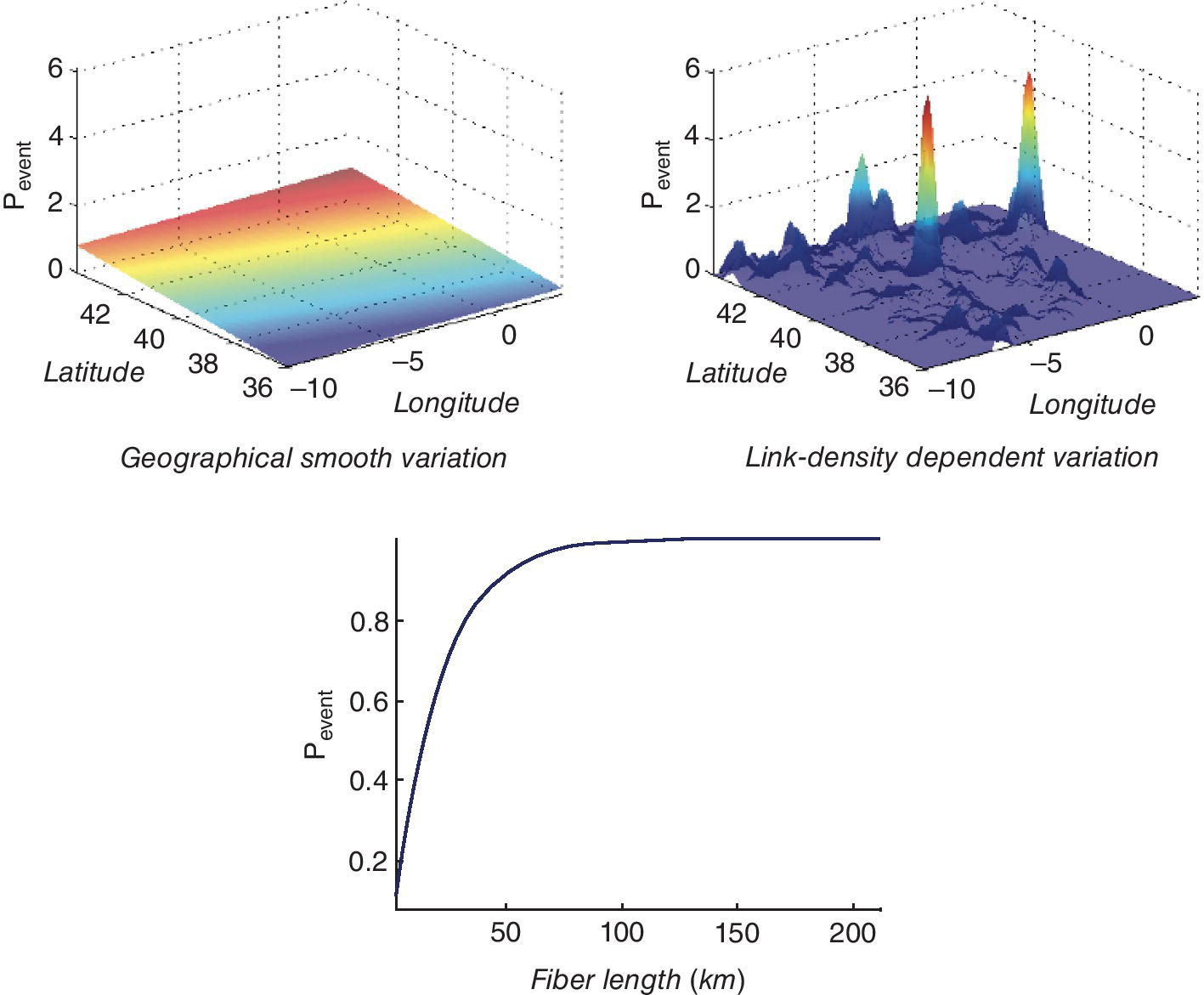
Figure 6.5 Surrogate model for link failure, and conditional components of the event model used.
The final probability of a link failure happening in a given link was given by an additive mixture of P1 and P2 spatial effects, and a multiplicative mixture of the spatial and the fiber length, as follows:
where c is a numerical normalization constant. We use the pdfs for defining the link events in terms of its geometric enter and its length (see their smooth variation in Figure 6.5) as follows:

Annual and Asymptotic Data Generation
We generated an annual event series given by a list of events that have been observed s[n] during the nth year, with Ny the number of annual events, given by sn, with n = 1, …, Ny, where for each event sn consists of a three‐tuple including the coordinates and length of each link. The annual event can be accumulated as follows:
allowing us to use a frequentist estimation of the event rates at each link:
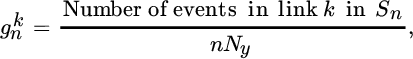
and it can be trivially shown to converge asymptotically to the actual event rate of the kth link; that is, ![]() . These asymptotic event probabilities were used as a benchmark for comparison of the estimated event probability given by learning from algorithms.
. These asymptotic event probabilities were used as a benchmark for comparison of the estimated event probability given by learning from algorithms.
Simulations with Surrogate Data
We used SVM and NN algorithms to estimate ![]() obtaining
obtaining ![]() ; that is, the frequentist estimation of the events for each link up to year n, given the inputs variables latitude, longitude, and fiber length, for each link (latk, lonk, Lk). Three different approaches were built using SVM algorithms with a Gaussian kernel in all of them: (1) SVM‐1 K uses just a single kernel for a vector containing the three input variables; (2) SVM‐2 K has two kernels, one for coordinates and one for length; and (3) SVM‐3 K using three kernels, one for each input variable. The results obtained were benchmarked with a generalized regression NN (GRNN) for function approximation (Demuth and Beale, 1993), which is also a nonlinear method and only requires a free parameter (Gaussian width) to be previously fixed.
; that is, the frequentist estimation of the events for each link up to year n, given the inputs variables latitude, longitude, and fiber length, for each link (latk, lonk, Lk). Three different approaches were built using SVM algorithms with a Gaussian kernel in all of them: (1) SVM‐1 K uses just a single kernel for a vector containing the three input variables; (2) SVM‐2 K has two kernels, one for coordinates and one for length; and (3) SVM‐3 K using three kernels, one for each input variable. The results obtained were benchmarked with a generalized regression NN (GRNN) for function approximation (Demuth and Beale, 1993), which is also a nonlinear method and only requires a free parameter (Gaussian width) to be previously fixed.
In the SVM models, a cross‐validation strategy (50% for training and 50% for validation) was applied to tune the free parameters; namely, the ones from the cost function (C, γ, ɛ), the width (σi) for each kernel and the relevance parameter λi. For each model, and using given free parameters, the MAE was calculated. We want to tune the set of free parameters that minimize the MAE. To that end, we started with fixed initial values for C, ε, σi, λi (i = 1, 2, or 3), we obtained the variation of MAEn with γ. We then fixed parameter γ to the value minimizing MAE[n], and we obtained the variation of MAEn as a function of C (while keeping the rest of the parameters to their fixed values). We continued this process until we explored all parameters.
The purpose of this surrogate data model consists of evaluating the methodology in a theoretic way, and comparing the estimated and the asymptotic results:

where ![]() is the estimated output after tuning the free parameters of the SVM with the training and validation sets, and
is the estimated output after tuning the free parameters of the SVM with the training and validation sets, and ![]() is the asymptotic corresponding value (n = 10 000 for Equation 6.90, as previously described).
is the asymptotic corresponding value (n = 10 000 for Equation 6.90, as previously described).
A similar procedure was followed for the GRNN, in which only the width parameter had to be searched in the rank σ ∈ (10−2, 10). The same considerations for the training and test set were followed. MAEn, and MAE![]() were also calculated for comparison purposes.
were also calculated for comparison purposes.
Nonobserved Events
In this application, we studied two possibilities for dealing with null events in the links of the networks: (1) including the set of samples for building the model (both training and testing) by giving them a null numerical value; and (2) excluding them from the training and validation process.
Results on Observed and Asymptotic Data
In this section we show results in terms of observed error and asymptotic error, which are given by MAEn, and MAE![]() respectively, when evaluating SVM‐1 K, SVM‐2 K, and SVM‐3 K, and an NN scheme using the GRNN. We used 10 independent realizations. Listing 6.6 shows how to obtain both the asymptotic model and when considering 2–20 years.
respectively, when evaluating SVM‐1 K, SVM‐2 K, and SVM‐3 K, and an NN scheme using the GRNN. We used 10 independent realizations. Listing 6.6 shows how to obtain both the asymptotic model and when considering 2–20 years.
Figure 6.6 shows the box plots for all the methods in the cases of including and not including the null events in the learning procedure. Panels (a) and (c) show the MAEn that should be observed with the events available up to year n, and it can be compared with the gold standard given by MAE![]() in panels (b) and (d) in terms of the box plots. Box plots use a box and whisker plot for the merit figures from each number of available years n in the conventional way, and have lines at the lower quartile, median, and upper quartile values. The plus sign represents the outliers.
in panels (b) and (d) in terms of the box plots. Box plots use a box and whisker plot for the merit figures from each number of available years n in the conventional way, and have lines at the lower quartile, median, and upper quartile values. The plus sign represents the outliers.
Figure 6.6 Simulations with surrogate data including null events into the training and test set (a, b) and without including them (c, d), after 10 independent realizations. (a, c) Box plot of MAEn (observed error in n years). (b, d) Box plot of MAE (asymptotic error, computed using Equation 6.91).
The observed error (i.e., the MAEn in n years) showed a too‐optimistic bias with very few years of events available, in particular, up to 5 years and 10 years respectively when considering and when not considering the null events in the training procedure. It also can be concluded that the asymptotic error (i.e., the MAE![]() ) clearly stabilized after an initial period of 10 years when considering the null events and of 5 years when not considering them. Finally, and overall, including the links with no events in the training procedure yielded lower asymptotic error in this case, which can be seen for instance in Figure 6.6b and d, with lower asymptotic error (MAE
) clearly stabilized after an initial period of 10 years when considering the null events and of 5 years when not considering them. Finally, and overall, including the links with no events in the training procedure yielded lower asymptotic error in this case, which can be seen for instance in Figure 6.6b and d, with lower asymptotic error (MAE![]() ) being obtained for 2–20 years for this approach. The synthetic model created for the surrogate data model is shown in Listing 6.7.
) being obtained for 2–20 years for this approach. The synthetic model created for the surrogate data model is shown in Listing 6.7.
It can be concluded that there are smooth partial relationships among variables, such as spatial or link fiber dependence. The methodology allows the study of complex interaction in HRCNs, increasing the accuracy with the number of availability events. We analyzed the effect of including or excluding the links with unobserved events in the training set. Finally, we benchmarked that better performance is obtained with SVM models, especially with few years of available data.
A Case Study
We also analyzed the historical data consisting of the events and the failures in the optical links from a real HRCN during 2 years. We used the same three input variables (longitude, latitude, and fiber length) to characterize each link. This real HRCN had a low number of observed events, 45 and 50 for S1 and S2 respectively. The same SVM algorithms were tested by using one, two, and three Gaussian kernels. Free parameters were tuned by using a cross‐validation technique, by randomly splitting the available data into training and validation subsets. We used MAE2 on the validation to assess the performance of the model. To give a statistical description of the accuracy, the estimations were repeated 200 times with different randomization.
Figure 6.7 shows the histograms of MAE2, in logarithmic units, for the three SVM algorithms. It is important to emphasize the bimodality in the error histograms, showing that there are two cluster of training subsets: one provides suboptimal results, whereas the other yields good performance. The MAE2 values for SVM‐1 K, SVM‐2 K, and SVM‐3 K algorithms were − 0.84, − 3.41, and − 3.42 respectively. The conclusion is that using two kernels provides a significant improvement, whereas the inclusion of a third kernel did not further enhance performance.

Figure 6.7 Histograms of the log(MAE2) in the validation sets for each SVM algorithm in the real case study.
6.3.4 Promotional Data
In this subsection, we first analyze from simulations the effect on the number of input features in different SR models. Then, we use SVM‐SR for an application example based on price promotions effects. In both cases, the use of bootstrap resampling for different model diagnoses is presented.
Effect of the Number of Input Features
One of the main limitations of SR is that, due to the nonparametric component of the model, its performance sensibly deteriorates with the number of input features (curse of dimensionality). For classification and regression problems, the SVM has been shown to be robust when working with high‐dimensional input spaces, in part due to the sparsity enforced on the solution. We present a simple simulation example that compares the behavior of SVM‐SR with the SR using the NW estimator (NW‐SR), in terms of the dimension of the input space.
The following model was used to generate the observations:

where σm and σd are the standard deviations of the ![]() and
and ![]() processes respectively; Q is an M × M constant matrix, whose elements are i.i.d. and drawn from a rectified Gaussian pdf, N(0, 1); β is a D × 1 vector, whose elements are i.i.d. and drawn from a uniform pdf
processes respectively; Q is an M × M constant matrix, whose elements are i.i.d. and drawn from a rectified Gaussian pdf, N(0, 1); β is a D × 1 vector, whose elements are i.i.d. and drawn from a uniform pdf
U(−1, 1); xm is an M × 1 random vector, drawn from an N(0, 2); xd is a D × 1 random vector, drawn from a Bernoulli pdf with 1‐probability of 0.5; and en is an N(0, 0.2) perturbation. Performance is evaluated for SVM‐SR and for NW‐SR, over a rank M ∈ (5, 40), and M = D. The training and the validation sets consist of 50 and 500 observations respectively. The experiment was repeated for 10 runs.
Figure 6.8 shows the runs‐averaged ρ for both methods. Whereas the performance of NW‐SR gets worse with the number of input variables, the error in SVM‐SR remains almost at the same level. For M > 30, performance is significantly different for both methods.

Figure 6.8 Quality score ρ for SVM‐SR and for NW‐SR in the simulation example as a function of the number of input features M.
Deal Effect Curve Estimation in Marketing
As a real application example, we describe next an approach to the analysis of the deal effect curve shape used in promotional analysis, by using the SVM‐SR in an available database (Soguero‐Ruiz et al., 2012). Our data set is constructed from store‐level scanner data of a Spanish supermarket for the period 2 January until 31 December 1999. The number of days in the data set is 304. To account for the effects of price discounts with promotional periods, data were represented on a daily basis. Ground coffee category is considered, as it is a storable product with a daily rate of sales. Brands occupying the major positions in the market (more than 80% of sales) and being sold on promotion were selected, leading to the selection of six brands: two national low‐priced brands (#1, #6), and four national high‐priced brands (#2 to #5), as seen in Table 6.3.
Table 6.3 Qualitative and quantitative prices (in pesetas) of coffee brands considered in the study.
| Brand | #1 | #2 | #3 | #4 | #5 | #6 |
| Price | Low | High | High | High | High | Low |
| Min–max | 159–225 | 189–259 | 185–240 | 189–249 | 187–235 | 157–195 |
The predicted variable is the sales units ![]() sold, at day i, i = 1, …, 304, for a certain brand k, k = 1, …, 5, in the category. Brand #6 was neither modeled nor considered in the model for the other brands, because it had no promotional discounts.
sold, at day i, i = 1, …, 304, for a certain brand k, k = 1, …, 5, in the category. Brand #6 was neither modeled nor considered in the model for the other brands, because it had no promotional discounts.
To capture the influence of the day of the week on the sales obtained on each day of the promotional period, we introduce two groups of dichotomic variables: for brand k and day i, variables ![]() are the indicators of the day of week (Monday (1) to Saturday (6)) during promotional periods, whereas
are the indicators of the day of week (Monday (1) to Saturday (6)) during promotional periods, whereas ![]() are the indicators of the day of week (Monday (7) to Saturday (12)) during nonpromotional periods in brand k. By distinguishing between both groups of variables, we can observe the gap in sales between promotional and nonpromotional periods due to the seasonal component.
are the indicators of the day of week (Monday (7) to Saturday (12)) during nonpromotional periods in brand k. By distinguishing between both groups of variables, we can observe the gap in sales between promotional and nonpromotional periods due to the seasonal component.
One of the characteristics of price discounts that researchers have commonly analyzed is the influence of promotional prices ending in the digit 9 in the sales obtained by the retailer (Blattberg and Neslin, 1993). To capture the influence of 9‐ending promotional prices in the sales obtained in the category, we introduced an indicator variable ![]() that takes the unit value when the promotional price of brand k is 9‐ending.
that takes the unit value when the promotional price of brand k is 9‐ending.
We also considered in our model the influence of the promotional price. In order to remove the effect of the price, the amplitude of the promotional discount was considered instead of the actual price, as proposed in Heerde et al. (2001). The price index, or ratio between the discounted price and the regular price, was introduced using a metric variable for each brand, ![]() , with m = 1, …, 6. Although we know that the retailer had used some kind of feature advertising and displays during the period considered, we do not have any information referring to their usage, so these important effects could not be included in the model.
, with m = 1, …, 6. Although we know that the retailer had used some kind of feature advertising and displays during the period considered, we do not have any information referring to their usage, so these important effects could not be included in the model.
For each SVM‐SR model, the free parameters were found using B = 20 bootstrap resamples for the R2 estimator. The observations were split into training (75%) and testing. For the best set of free parameters, the CI for merit figures R2, ρ, and the CI for parametric variables were obtained (95% content). As collinearity between metric variables for price indexes and dichotomic variables for promotional day of the week was suspected, a test for the exclusion of the metric variables was performed. Interaction effects between pairs of price indexes were obtained for each model.
Models for all the brands reached a significant R2 (see Table 6.4). Two examples of model fitting are shown in Figure 6.9a and d for a high‐quality and a low‐quality brand respectively. Their corresponding CIs for the parametric variables are depicted in Figure 6.9b and e. It can be observed that the weekly pattern is significantly different in both of them, with the amplitude of the amplitude of the promotional oscillations being greater than the nonpromotional. The highest rates of sale correspond to promotional weekend periods. This behavior is present in all the other models (not shown). With respect to the 9‐ending effect, it significantly increased the sales in brand #1, but not in brand #2. The self‐effects of the in brand #2. The self‐effects of the promotion are shown in Figure 6.9c and f. The increment of sales in brand #2 (high quality).
Table 6.4 Significance for the inclusion of metric variables.
| R2 | CI S2 | ρ | CI ϱ | |
| #1 | 0.78† | (0.27,0.65) | 2.61† | (2.84,4.40) |
| #2 | 0.85† | (0.61,0.83) | 5.54† | (5.66,8.51) |
| #3 | 0.84† | (0.55,0.70) | 6.37† | (6.57,9.76) |
| #4 | 0.82† | (0.39,0.76) | 3.00† | (3.02,4.95) |
| #5 | 0.69 | (0.43,0.76) | 1.85 | (1.77,2.34) |
† indicates significant at the 95% level.

Figure 6.9 Examples of results for deal effect curve analysis, showing model fitting (a), CI for parametric variables and intercept (b), and self‐effect of discounts (c) for brands #1 (upper row) and #2 (middle row). Cross‐item effect are shown for brand #1 on brand #3 model (a) and for brand #5 on brand #4 model. Confidence bands for averaged output are shown in brand #2 (detail).
Table 6.4 shows the results for the test of significance of the price indexes in the model. In all but one (brand #5), nonparametric variables were relevant to explain the sales jointly with the weekly oscillations. This can be seen as two different effects due to the promotion: an increase in the average level of sales (function of the price index), and a fixed increase in the weekly oscillations amplitude.
Once the relevance of the price indexes has been established, it is worth exploring the complex, nonlinear relationship among them. We only describe here two examples. Figure 6.9 g shows the cross‐effects of brand #1 on brand #3 model. For the simultaneous promotion situation, brand in a stronger competence than brand #3, as sales of the later fall. However, Figure 6.9 h illustrates a weaker competence, as promotion in brand #4 increases the sales even despite the simultaneous promotion in brand #5.
6.3.5 Spatial and Temporal Antenna Array Kernel Processing
We benchmarked in Martínez‐Ramón et al. (2006) the kernel temporal reference (SVM‐TR) and the spatial reference (SVM‐SRef) array processors, together with their kernel LS counterparts (kernel‐TR and kernel‐SRef) and to the linear with temporal reference (MMSE) and with spatial reference (MVDM). We used a Gaussian kernel in all cases. The scenario consisted of a multiuser environment with four users, one being the desired user and the rest being the interferences. The modulated signals were independent QPSK. The noise was assumed to be thermal, simulated by additive white Gaussian noise. The desired signal was structured in bursts containing 100 training symbols, followed by 1000 test symbols. Free parameters were chosen in the first experiment and fixed after checking the stability of the algorithms with respect to them.
The BER was measured as a function of kernel parameter δ for arrays of five and seven elements, in an environment of three interferences from angles of arrival of 10°, 20° and − 10°, and unitary amplitudes, while the desired signal came from an angle of arrival of 0° with the same amplitude as the interferences. Results in Figure 6.10 show the BER as a function of the RBF kernel width for the temporal and spatial reference SVM algorithms.

Figure 6.10 BER performance as a function of RBF kernel parameter δ, of the TR (squares) and the SR (circles) in an array of seven (top) and five (bottom) elements and with three interferent signals. Continuous line corresponds to the performance of the linear algorithms.
These results were compared with the temporal and spatial kernel LS algorithms (i.e., kernel‐TR and ‐SR), and for seven and five array‐elements. The noise power was of − 1 dB for seven elements and − 6 dB for five elements. The results of the second experiment are shown in Figure 6.11. The experiment measured the BER of the four nonlinear processors as a function of the thermal noise power in an environment with three interfering signals from angles of arrival of − 10°, 10°, and 20°. The desired signal direction of arrival was 0°.

Figure 6.11 BER performance as a function of thermal noise power for linear algorithms, SVM SVM‐TR, SVM‐SR, Kernel‐TR, and Kernel‐SR.
Performance was compared with the linear MVDR and MMSE algorithms. All nonlinear approaches showed similar performance, and an improvement of several decibels with respect to the linear algorithms. SVM approaches showed similar or slightly better performance than nonlinear LS algorithms, and with lower test computational burden due to their sparseness properties.
6.4 Questions and Problems
- Exercise 6.4.1 Propose a data model in which composite kernels can provide an RKHS signal model. You can search in classic statistics, in DSP literature, or in machine learning literature.
- Exercise 6.4.2 Propose an example of signal or image analysis where you need to combine different sources of data, and hence where the use of a composite kernel can be advantageous.
- Exercise 6.4.3 Program the simple simulation example used to compare NW with SVM for SR in terms of the number of input features.
- Exercise 6.4.4 With the previous example, adjust the NW estimator and the SVM estimator. Are your results consistent with the ones shown in the chapter?
- Exercise 6.4.5 Provide CIs for the statistical estimates described in the bootstrap resampling section for this same synthetic problem.