
9
Adaptive Kernel Learning for Signal Processing
9.1 Introduction
Adaptive filtering is a central topic in signal processing. An adaptive filter is a filter structure provided with an adaptive algorithm that tunes the transfer function, typically driven by an error signal. Adaptive filters are widely applied in nonstationary environments because they can adapt their transfer function to match the changing parameters of the system that generates the incoming data (Hayes 1996 ; Widrow et al. 1975). They have become ubiquitous in current DSP, mainly due to the increase in computational power and the need to process streamed data. Adaptive filters are now routinely used in all communication applications for channel equalization, array beamforming, or echo cancellation, to cite just a few, and in other areas of signal processing, such as image processing or medical equipment.
By applying linear adaptive filtering principles in the kernel feature space, powerful nonlinear adaptive filtering algorithms can be obtained. This chapter introduces the wide topic of adaptive signal processing, and it explores the emerging field of kernel adaptive filtering (KAF). Its orientation is different from the preceding ones, as adaptive processing can be used in a variety of scenarios. Attention is paid to kernel LMS and RLS algorithms, to previous taxonomies of adaptive kernel methods, and to emergent kernel methods for online and recursive KAF. MATLAB code snippets are included as well to illustrate the basic operations of the most common kernel adaptive filters. Tutorial examples are provided on applications, including chaotic time‐series prediction, respiratory motion prediction, and nonlinear system identification.
9.2 Linear Adaptive Filtering
Let us first define some basic concepts of linear adaptive filtering theory. The goal of adaptive filtering is to model an unknown, possibly time‐varying system by observing the inputs and outputs of this system over time. We will denote the input to the system on time instant n as xn, and its output as dn. The input signal xn is assumed to be zero‐mean. We represent it as a vector, and it will often represent a time‐delay vector of L taps of a signal xn on time instant n as xn = [xn, xn−1, …, xn−L+1]T.
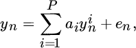
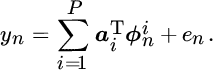
A diagram for a linear adaptive filter is depicted in Figure 9.1. The input to the adaptive filter at time instant n is xn, and its response yn is obtained through the following linear operation:
where H is the Hermitian operator.
Figure 9.1 A linear adaptive filter for system identification.
Linear adaptive filtering follows the online learning framework, which consists of two basic steps that are repeated at each time instant n. First, the online algorithm receives an observation xn for which it calculates the estimated image yn, based on its current estimate of wn. Next, the algorithm receives the desired output dn (also known as a symbol in communications), which allows it to calculate the estimation error en = dn − yn and update its estimate for wn. In some situations dn is known a priori; that is, the received signal xn is one of a set of training signals provided with known labels. The procedure is then called supervised. When dn belongs to a finite set of quantized labels, and it can be assumed that the error will be likely much smaller than the quantization step or minimum Euclidean distance between labels, the desired label is estimated by quantizing yn to the closest label. In these cases, the algorithm is called decision directed.
9.2.1 Least Mean Squares Algorithm
The classical adaptive optimization techniques have their roots in the theoretical approach called the steepest‐descent algorithm. Assume that the expectation of the squared error signal, ![]() can be computed. Since this error is a function of the vector wn, the idea of the algorithm is to modify this vector toward the direction of the steepest descent of Jn. This direction is just opposite to its gradient ∇wJn. Indeed, assuming complex stationary signals, the error expectation is
can be computed. Since this error is a function of the vector wn, the idea of the algorithm is to modify this vector toward the direction of the steepest descent of Jn. This direction is just opposite to its gradient ∇wJn. Indeed, assuming complex stationary signals, the error expectation is

where Rxx is the signal autocorrelation matrix, pxd is the cross‐correlation vector between the signal and the filter output, and ![]() is the variance of the system output. Its gradient with respect to vector wn is expressed as
is the variance of the system output. Its gradient with respect to vector wn is expressed as
The adaptation rule based on steepest descent thus becomes
where η is the step size or learning rate of the algorithm.
The LMS algorithm, introduced by Widrow in 1960 (Widrow et al., 1975), is a very simple and elegant method of training a linear adaptive system to minimize the MSE that approximates the gradient ∇wJn using an instantaneous estimate of the gradient. From Equation 9.3, an approximation can be written as
Using this approximation in Equation 9.4 leads to the well‐known stochastic gradient descent update rule, which is the core of the LMS algorithm:

This optimization procedure is also the basis for tuning nonlinear filter structures such as NNs (Haykin, 2001) and some of the kernel‐based adaptive filters discussed later in this chapter. A detailed analysis including that of convergence and misadjustment is given in Haykin (2001). The MATLAB code for the LMS training step on a new data pair (x, d) is displayed in Listing 9.1.
Under the stationarity assumption, the LMS algorithm converges to the Wiener solution in mean, but the weight vector wn shows a variance that converges to a value that is a function of η. Therefore, low variances are only achieved at low adaptation speed. A more sophisticated approach with faster convergence is found in the the RLS algorithm.
9.2.2 Recursive Least‐Squares Algorithm
The RLS algorithm was first introduced in 1950 (Plackett, 1950). In a stationary scenario, it converges to the Wiener solution in mean and variance, improving also the slow rate of adaptation of the LMS algorithm. Nevertheless, this gain in convergence speed comes at the price of a higher complexity, as we will see later.
Recursive Update
The basis of the RLS algorithm consists of recursively updating the vector w that minimizes a regularized version of the cost function Jn:

where δ is a positive constant regularization factor. The regularization factor penalizes the squared norm of the solution vector so that this solution does not apply too much weight to any specific dimension.1 The solution that minimizes the LS cost function (9.7) is well known and given by
The regularization δ guarantees that the inverse in Equation 9.8 exists. In the absence of regularization (i.e., for δ = 0), the solution requires one to invert the matrix Rxx, which may be rank deficient. For a detailed derivation of the RLS algorithm we refer the reader to Haykin (2001) and Sayed (2003). In the following, we will provide its update equations and a short discussion of its properties compared with LMS.
We denote the autocorrelation matrix for the data x1 till xn as Rn:

RLS requires the introduction of an inverse autocorrelation matrix Pn, defined as
At step n − 1 of the recursion, the algorithm has processed n − 1 data, and its estimate wn−1 is the optimal solution for minimizing the squared cost function (Equation 9.7) at time step n − 1. When a new datum xn is obtained, the inverse autocorrelation matrix is updated as
where gn is the gain vector of the RLS algorithm:
The update of the solution itself reads
in which en represents the usual prediction error ![]() . The RLS algorithm starts by initializing its solution to w0 = 0, and the estimate of the inverse autocorrelation matrix Pn to P0 = δ−1I. Then, it recursively updates its solution by including one datum xi at a time and performing the calculations from Equations 9.11–9.13. Owing to the matrix multiplications involved in the RLS updates, the computational complexity per time step for RLS is quadratic in terms of the data dimension,
. The RLS algorithm starts by initializing its solution to w0 = 0, and the estimate of the inverse autocorrelation matrix Pn to P0 = δ−1I. Then, it recursively updates its solution by including one datum xi at a time and performing the calculations from Equations 9.11–9.13. Owing to the matrix multiplications involved in the RLS updates, the computational complexity per time step for RLS is quadratic in terms of the data dimension, ![]() , while the LMS algorithm has only linear complexity,
, while the LMS algorithm has only linear complexity, ![]() .
.
Exponentially Weighted Recursive Least‐Squares
The RLS algorithm takes into account all previous data when it updates its solution with a new datum. This kind of update yields a faster convergence than LMS, which guides its update based only on the performance on the newest datum. Nevertheless, by guaranteeing that its solution is valid for all previous data, the RLS algorithm is in essence looking for a stationary solution, and thus it cannot adapt to nonstationary scenarios, where a tracking algorithm is required. LMS, on the other hand, deals correctly with nonstationary scenarios, thanks to the instantaneous nature of its update, which forgets older data and only adapts to the newest datum.
A tracking version of RLS can be obtained by including a forgetting factor λ ∈ (0, 1] in its cost function as follows:
The resulting algorithm is called exponentially weighted RLS (Haykin, 2001 ; Sayed, 2003). The inclusion of the forgetting factor assigns lower weights to older data, which allows the algorithm to adapt gradually to changes. The update for the inverse autocorrelation matrix becomes
and the new gain vector becomes
The MATLAB code for the training step of the exponentially weighted RLS algorithm is displayed in Listing 9.2.
Recursive estimation algorithms play a crucial role for many problems in adaptive control, adaptive signal processing, system identification, and general model building and monitoring problems (Ljung, 1999). In the signal‐processing literature, great attention has been paid to their efficient implementation. Linear AR models require relatively few parameters and allow closed‐form analysis, while ladder or lattice implementation of linear filters has long been studied in signal theory. However, when the system generating the data is driven by nonlinear dynamics, the model specification and parameter estimation problems increase their complexity, and hence nonlinear adaptive filtering becomes strictly necessary.
Note that, in the field of control theory, a range of sequential algorithms for nonlinear filtering have been proposed since the 1960s, notably the extended KF (Lewis et al., 2007) and the unscented KF (Julier and Uhlmann, 1996), which are both nonlinear extensions of the celebrated KF (Kalman, 1960), and particle filters (Del Moral, 1996). These methods generally require knowledge of a state‐space model, and while some of them are related to adaptive filtering, we will not deal with them explicitly in this chapter.
9.3 Kernel Adaptive Filtering
The nonlinear filtering problem and the online adaptation of model weights were first addressed by NNs in the 1990s (Dorffner 1996 ; Narendra and Parthasarathy 1990). Throughout the last decade, a great interest has been devoted to developing nonlinear versions of linear adaptive filters by means of kernels (Liu et al., 2010). The goal is to develop machines that learn over time in changing environments, and at the same time adopt the nice characteristics of convexity, convergence, and reasonable computational complexity, which was not successfully implemented in NNs.
Kernel adaptive filtering aims to formulate the classic linear adaptive filters in RKHS, such that a series of convex LS problems is solved. Several basic kernel adaptive filters can be obtained by applying a linear adaptive filter directly on the transformed data, as illustrated in Figure 9.2. This requires the reformulation of scalar‐product‐based operations in terms of kernel evaluations. The resulting algorithms typically consist of algebraically simple expressions, though they feature powerful nonlinear filtering capabilities. Nevertheless, the design of these online kernel methods requires dealing with some of the challenges that typically arise when dealing with kernels, such as overfitting and computational complexity issues.

Figure 9.2 A kernel adaptive filter for nonlinear system identification.
In the following we will discuss two families of kernel adaptive filters in detail, namely KLMS and kernel RLS (KRLS) algorithms. Several related kernel adaptive filters will be reviewed briefly as well.
9.4 Kernel Least Mean Squares
The early approach to kernel adaptive filtering introduced a kernel version of the celebrated ADALINE in Frieß and Harrison (1999), though this method was not online. Kivinen et al. (2004) proposed an algorithm to perform stochastic gradient descent in RKHS: the so‐called naive online regularized risk minimization algorithm (NORMA) introduces a regularized risk that can be solved online and can be shown to be equivalent to a kernel version of leaky LMS, which itself is a regularized version of LMS.
9.4.1 Derivation of Kernel Least Mean Squares
As an illustrative guiding example of a kernel adaptive filter, we will take the kernelization of the standard LMS algorithm, known as KLMS (Liu et al., 2008). The approach employs the traditional kernel trick. Essentially, a nonlinear function ϕ(⋅) maps the data xn from the input space to ϕ(xn) in the feature space. Let ![]() be the weight vector in this space such that the filter output is
be the weight vector in this space such that the filter output is ![]() , where
, where ![]() is the estimate of
is the estimate of ![]() at time instant n. Note that we will be taking scalar products of real‐valued vectors from now on. Given a desired response dn, we wish to minimize squared loss,
at time instant n. Note that we will be taking scalar products of real‐valued vectors from now on. Given a desired response dn, we wish to minimize squared loss, ![]() , with respect to
, with respect to ![]() . Similar to Equation 9.6, the stochastic gradient descent update rule obtained reads
. Similar to Equation 9.6, the stochastic gradient descent update rule obtained reads
By initializing the solution as ![]() (and hence e0 = d0 = 0), the solution after n iterations can be expressed in closed form as
(and hence e0 = d0 = 0), the solution after n iterations can be expressed in closed form as
By exploiting the kernel trick, one obtains the prediction function
where x* represents an arbitrary input datum and K(⋅, ⋅) is the kernel function; for instance, the commonly used Gaussian kernel ![]() with kernel width σ. Note that the weights
with kernel width σ. Note that the weights ![]() of the nonlinear filter are not used explicitly in the KLMS algorithm. Also, since the present output is determined solely by previous inputs and all the previous errors, it can be readily computed in the input space. These error samples are similar to innovation terms in sequential state estimation (Haykin, 2001), since they add new information to improve the output estimate. Each new input sample results in an output, and hence a corresponding error, which is never modified further and incorporated in the estimate of the next output. This recursive computation makes KLMS especially useful for online (adaptive) nonlinear signal processing.
of the nonlinear filter are not used explicitly in the KLMS algorithm. Also, since the present output is determined solely by previous inputs and all the previous errors, it can be readily computed in the input space. These error samples are similar to innovation terms in sequential state estimation (Haykin, 2001), since they add new information to improve the output estimate. Each new input sample results in an output, and hence a corresponding error, which is never modified further and incorporated in the estimate of the next output. This recursive computation makes KLMS especially useful for online (adaptive) nonlinear signal processing.
Liu et al. (2008) showed that the KLMS algorithm is well posed in RKHS without the need of an extra regularization term in the finite training data case, because the solution is always forced to lie in the subspace spanned by the input data. The lack of an explicit regularization term leads to two important advantages. First of all, it has a simpler implementation than NORMA, as the update equations are straightforward kernel versions of the original linear ones. Second, it can potentially provide better results because regularization biases the optimal solution. In particular, it was shown that a small enough step size can provide a sufficient “self‐regularization” mechanism. Moreover, since the space spanned by the mapped samples is possibly infinite dimensional, the projection error of the desired signal dn could be very small, as is well known from Cover’s theorem (Haykin, 1999). On the downside, the speed of convergence and the misadjustment also depend upon the step size. As a consequence, they conflict with the generalization ability.
9.4.2 Implementation Challenges and Dual Formulation
Another important drawback of the KLMS algorithm becomes apparent when analyzing its update, Equation 9.19. In order to make a prediction, the algorithm requires storing all previous errors ei and all processed input data xi, for ![]() . In online scenarios, where data are continuously being received, the size of the KLMS network will continuously grow, posing implementation challenges. This becomes even more evident if we recast the weight update from Equation 9.17 into a more standard filtering formulation, by relying on the representer theorem (Schölkopf et al., 2001). This theorem states that the solution wℋ,n can be expressed as a linear combination of the transformed input data:
. In online scenarios, where data are continuously being received, the size of the KLMS network will continuously grow, posing implementation challenges. This becomes even more evident if we recast the weight update from Equation 9.17 into a more standard filtering formulation, by relying on the representer theorem (Schölkopf et al., 2001). This theorem states that the solution wℋ,n can be expressed as a linear combination of the transformed input data:

This allows the prediction function to be written as the familiar kernel expansion
The expansion coefficients αi are called the dual variables and the reformulation of the filtering problem in terms of αi is called the dual formulation. The update from Equation 9.17 now becomes
and after multiplying both sides with the new datum ϕ(xn) and adopting a vector notation, we obtain
where αn = [α1, α2, …, αn]T, the vector kn contains the kernels of the n data and the newest point, kn = [K(x1, xn), K(x2, xn), …, K(xn, xn)], and knn = K(xn, xn). KLMS resolves this relationship by updating αn as

The MATLAB code for the complete KLMS training step on a new data pair (x, d) is displayed in Listing 9.3.
The update in Equation 9.24 emphasizes the growing nature of the KLMS network, which precludes its direct implementation in practice. In order to design a practical KLMS algorithm, the number of terms in the kernel expansion in Equation 9.21 should stop growing over time. This can be achieved by implementing an online sparsification technique, whose aim is to identify terms in the kernel expansion that can be omitted without degrading the solution. We will discuss several different sparsification approaches in Section 9.7. Finally, observe that the computational complexity and memory complexity of the KLMS algorithm are both linear in terms of the number of data it stores, ![]() . Recall that the complexity of the LMS algorithm is also linear, though not in terms of the number of data but in terms of the data dimension.
. Recall that the complexity of the LMS algorithm is also linear, though not in terms of the number of data but in terms of the data dimension.
9.4.3 Example on Prediction of the Mackey–Glass Time Series
We demonstrate the online learning capabilities of the KLMS kernel adaptive filter by predicting the Mackey–Glass time series, which is a classic benchmark problem (Liu et al., 2010). The Mackey–Glass time series is well known for its strong nonlinearity. It corresponds to a high‐dimensional chaotic system, and its output is generated by the following time‐delay differential equation:

We focus on the sequence with parameters b = 0.1, a = 0.2, and time delay Δ = 30, better known as the MG30 time series. The prediction problem consists of predicting the nth sample, given all samples of the time series up till the n − 1th sample.
Time‐series prediction with kernel adaptive filters is typically performed by considering a time‐delay vector xn = [xn, xn−1, …, xn−L+1]T as the input and the next sample of the time series as the desired output, dn = xn+1. This approach casts the prediction problem into the well‐known filtering framework.2 Prediction of several steps ahead can be obtained by choosing a prediction horizon h > 1, and dn = xn+h. For time series generated by a deterministic process, a principled tool to find the optimal embedding is Takens’ theorem (Takens, 1981). In the case of the MG30 time series, Takens’ theorem indicates that the optimal embedding is around L = 7 (Van Vaerenbergh et al., 2012a).
We consider 500 samples for online training of the KLMS algorithm and use the next 100 data for testing. The step size of KLMS is fixed to 0.2, and we use the Gaussian kernel with σ = 1. Figure 9.3 displays the prediction results after 500 training steps. The left plot shows the learning curve of the algorithm, obtained as the MSE of the prediction on the test set, at each iteration of the online training process. As a reference, we include the learning curve of the linear LMS algorithm with a suitable step size. The right plot shows the 100 test samples of the original time series, as the full line, and KLMS’ prediction on these test samples after 500 training steps. These predictions are calculated by evaluating the prediction equation (Equation 9.19) on the test samples. The code for this experiment and all subsequent ones is included in the accompanying material in the book webpage.
Figure 9.3 KLMS predictions on the Mackey–Glass time series. Left: learning curve over 500 training iterations. Right: test samples of the Mackey–Glass time‐series and the predictions provided by KLMS.
9.4.4 Practical Kernel Least Mean Squares Algorithms
In the Mackey–Glass experiment described, the KLMS algorithm requires to store 500 coefficients αi and the 500 corresponding data xi. The stored data xi are referred to as its dictionary. If the online learning process were to continue indefinitely, the algorithm would require ever‐growing memory and computation per time step. This issue was identified as a major roadblock early on in the research on kernel adaptive filters, and it has led to the development of several procedures to slow down the dictionary growth by sparsifying the dictionary.
A sparsification procedure based on Gaussian elimination steps on the Gram matrix was proposed in Pokharel et al. (2009). This method is successful in limiting the dictionary size in the nth training step to some m < n, but in order to do so it requires ![]() complexity, which defeats the purpose of using a KLMS algorithm.
complexity, which defeats the purpose of using a KLMS algorithm.
Kernel Normalized Least Mean Squares and Coherence Criterion
Around the same time the KLMS algorithm was published, a kernelized version of the affine projection algorithm was proposed (Richard et al., 2009). Affine projection algorithms hold the middle ground between LMS and RLS algorithms by calculating an estimate of the correlation matrix based on the p last data. For p = 1 the algorithm reduces to a kernel version of the normalized LMS algorithm (Haykin, 2001), called kernel normalized least‐mean squares (KNLMS), and its update reads

Note that this algorithm updates all coefficients in each iteration. This is in contrast to KLMS, which updates just one coefficient.
The kernel affine projection and KNLMS algorithms introduced in Richard et al. (2009) also included an efficient dictionary sparsification procedure, called the coherence criterion. Coherence is a measure to characterize a dictionary in sparse approximation problems, defined in a kernel context as
The coherence of a dictionary will be large if it contains two bases xi and xj that are very similar, in terms of the kernel function. Owing to their similarity, such bases contribute almost identical information to the algorithm, and one of them may be considered redundant. The online dictionary sparsification procedure based on coherence operates by only including a new datum xn into the current dictionary ![]() if it maintains the dictionary coherence below a certain threshold:
if it maintains the dictionary coherence below a certain threshold:
If the new datum fulfills this criterion, it is included in the dictionary, and the KNLMS coefficients are updated through Equation 9.26. If the coherence criterion in Equation 9.28 is not fulfilled, the new datum is not included in the dictionary, and a reduced update of the KNLMS coefficients is performed:

This update does not increase the number of coefficients, and therefore it maintains the algorithm’s computational complexity fixed during that iteration. The MATLAB code for the complete KNLMS training step on a new data pair (x, d) is displayed in Listing 9.4.
The coherence criterion is computationally efficient, in that it has a complexity that does not exceed that of the kernel adaptive filter itself, and it has been demonstrated to be successful in practical situations (Van Vaerenbergh and Santamaría, 2013).
Quantized Kernel Least Mean Squares
Recently, a KLMS algorithm was proposed that combines elements from the original KLMS algorithm and the coherence criterion, called quantized KLMS (QKLMS) (Chen et al., 2012). In particular, when the sparsification criterion decides to include a datum into the dictionary, the algorithm updates its coefficients as follows:

When the datum does not fulfill the coherence criterion, it is not included in the dictionary. Instead, the closest dictionary element is retrieved, and the corresponding coefficient is updated as follows
where j is the dictionary index of the element that is closest. Though conceptually very simple, this algorithm obtains state‐of‐the‐art results in several applications when only a low computational budget is available. The MATLAB code for the complete QKLMS training step on a new data pair (x, d) is displayed in Listing 9.5.
9.5 Kernel Recursive Least Squares
In linear adaptive filtering, the RLS algorithm represents an alternative to LMS, with faster convergence and typically lower bias, at the expense of a higher computational complexity. RLS is obtained by designing a recursive solution to the LS problem. Analogously, a recursive solution can be designed for the KRR problem, yielding KRLS algorithms.
9.5.1 Kernel Ridge Regression
Let us review the KRR algorithm seen in Chapter 8. This will be the key to obtain the kernel‐based version of the regularized LS cost function in Equation 9.7. We essentially first transform the data into the kernel feature space:

where we have applied the kernel trick to obtain the second equality. Here, vector d contains the n desired values, d = [d1, d2, …, dn]T, and K is the kernel matrix with elements Kij = K(xi, xj). Equation 9.32 represents the KRR problem (Saunders et al., 1998), and its solution is given by
The prediction for a new datum x* is obtained as
9.5.2 Derivation of Kernel Recursive Least Squares
The KRLS algorithm (Engel et al., 2004) formulates a recursive procedure to obtain the solution of the regression problem in Equation 9.32 in the absence of regularization, λ = 0. Without regularization, the solution (Equation 9.33) reads
KRLS guarantees the invertibility of the kernel matrix K by excluding those data xi from the dictionary that are linearly dependent on the already included data, in the feature space. As we will see, this is achieved by applying a specific online sparsification procedure, which guarantees both that K is invertible and that the algorithm’s dictionary stays compact.
Assume the solution after processing n − 1 data is available, given by
In the next iteration n, a new data pair (xn, dn) is received and we wish to obtain the new solution αn by applying a low‐complexity update on the previous solution (Equation 9.36). We first calculate the predicted output
and we obtain the a‐priori error for this datum, en = dn − yn. The updated kernel matrix can be written as

By introducing the variables
and
the update for the inverse kernel matrix can be written as

Equation 9.41 is obtained by applying the Sherman–Morrison–Woodbury formula for matrix inversion; see, for instance, Golub and Van Loan (1996). Finally, the updated solution αn is obtained as

Equations 9.41 and 9.42 are efficient updates that allow one to obtain the new solution in ![]() time and memory, based on the previous solution. Directly applying Equation 9.35 at iteration n would require
time and memory, based on the previous solution. Directly applying Equation 9.35 at iteration n would require ![]() cost, so the recursive procedure is preferred in online scenarios. A detailed derivation of this result can be found in Engel et al. (2004) and Van Vaerenbergh et al. (2012b).
cost, so the recursive procedure is preferred in online scenarios. A detailed derivation of this result can be found in Engel et al. (2004) and Van Vaerenbergh et al. (2012b).
Online Sparsification by Approximate Linear Dependency
The KRLS algorithm from Engel et al. (2004) follows the described recursive solution. In order to slow down the dictionary growth, shown in Equations 9.41 and 9.42, it introduces a sparsification criterion based on approximate linear dependency (ALD). According to this criterion, a new datum xn should only be included in the dictionary if ϕ(xn) cannot be approximated sufficiently well in feature space by a linear combination of the already present data.
Given a dictionary ![]() of data xj and a new training point xn, we need to find a set of coefficients a = [a1, a2, …, am]T that satisfy the ALD condition
of data xj and a new training point xn, we need to find a set of coefficients a = [a1, a2, …, am]T that satisfy the ALD condition
where m is the cardinality of the dictionary. Interestingly, it can be shown that these coefficients are already calculated by the KRLS update itself, and they are available at each iteration n as ![]() , see Equation 9.39. The ALD condition can therefore be verified by simply comparing γn with the ALD threshold:
, see Equation 9.39. The ALD condition can therefore be verified by simply comparing γn with the ALD threshold:
If γn > ν, then we must add the newest datum xn to the dictionary, ![]() , before updating the solution through Equation 9.42. If γn ≤ ν then the datum xn is already represented sufficiently well by the dictionary. In this case the dictionary is not expanded,
, before updating the solution through Equation 9.42. If γn ≤ ν then the datum xn is already represented sufficiently well by the dictionary. In this case the dictionary is not expanded, ![]() , and a reduced update of the solution is performed; see Engel et al. (2004) for details. The MATLAB code for the complete KRLS training step on a new data pair (x, d) is displayed in Listing 9.6.
, and a reduced update of the solution is performed; see Engel et al. (2004) for details. The MATLAB code for the complete KRLS training step on a new data pair (x, d) is displayed in Listing 9.6.
9.5.3 Prediction of the Mackey–Glass Time Series with Kernel Recursive Least Squares
The update equations for KRLS require substantially more computation than KLMS. In particular, KRLS has quadratic complexity, ![]() , in terms of its dictionary size, and KLMS has linear complexity,
, in terms of its dictionary size, and KLMS has linear complexity, ![]() . On the other hand, KRLS has faster convergence and lower bias. We illustrate these properties by applying KRLS on the Mackey–Glass prediction experiment from Section 9.4.3.
. On the other hand, KRLS has faster convergence and lower bias. We illustrate these properties by applying KRLS on the Mackey–Glass prediction experiment from Section 9.4.3.
Figure 9.4 shows the results of training the KRLS algorithm on the Mackey–Glass time series. KRLS is applied with a Gaussian kernel with σ = 1, and its precision parameter was fixed to ν = 10−4. The left plot compares the learning curves of KLMS and KRLS, demonstrating a slightly faster initial convergence rate for KRLS, after which the algorithm converges to a much lower MSE than KLMS. The low bias is also visible in the right plot, which shows the prediction results on the test data.

Figure 9.4 KRLS predictions on the Mackey–Glass time series. Left: learning curve over 500 training iterations, including comparison with KLMS. Right: test samples and KRLS predictions.
9.5.4 Beyond the Stationary Model
An important limitation of the KRLS algorithm is that it always assumes a stationary model, and therefore it cannot track changes in the true underlying data model. This is a somewhat odd property for an adaptive filter, though note that this is also the case for the original RLS algorithm; see Section 9.2.2. In order to enable tracking and make a truly adaptive KRLS algorithm, several modifications have been presented in the literature. An exponentially weighted KRLS algorithm was proposed by including a forgetting factor, and an extended KRLS algorithm was designed by assuming a simple state‐space model, though both algorithms show numerical instabilities in practice (Liu et al., 2010). In the following we briefly discuss two different approaches that successfully allow KRLS to adapt to changing environments.
Sliding‐Window Kernel Recursive Least Squares
The KRLS algorithm summarizes past information into a compact formulation that does not allow easy manipulation. For instance, there does not exist a straightforward manner to include a forgetting factor to exclude the influence of older data.
Van Vaerenbergh et al. (2006) proposed sliding‐window KRLS (SW‐KRLS). This algorithm stores a window of the last m data as its dictionary, and once a datum is older than m time steps it is simply discarded. In each step the algorithm adds the new datum and discards the oldest datum, leading to a sliding‐window approach. The algorithm stores the inverse regularized kernel matrix, (Kn + λI)−1, calculated on its current dictionary, and a vector of the corresponding desired outputs, dn. By storing these variables it can calculate the solution vector by simply evaluating αn = (Kn + λI)−1dn; see Equations 9.33 and 9.34.
The inverse kernel matrix is updated in two steps. First, the new datum is added, which requires expanding the matrix with one row and one column. This is carried out by performing the operation from Equation 9.41, similar to in the KRLS algorithm. Second, the oldest datum is discarded, which requires removing one row and column from the inverse kernel matrix. This can be achieved by writing the kernel matrix and its inverse as follows:

after which the inverse (regularized) kernel matrix is found as
Details can be found in Van Vaerenbergh et al. (2006). Figure 9.5 illustrates the kernel matrix updates when using a sliding window, compared with the classical growing‐window approach of KRLS. The MATLAB code for the SW‐KRLS training step on a new data pair (x, d) is displayed in Listing 9.7.
Figure 9.5 Different forms of updating the kernel matrix during online learning. In KRLS‐type algorithms the update involves calculating the inverse of each kernel matrix, given the inverse of the previous matrix. Left: growing kernel matrix, as constructed in KRLS (omitting sparsification for simplicity). Right: sliding‐window kernel matrix of a fixed size, as constructed in SW‐KRLS.
SW‐KRLS is a conceptually very simple algorithm that obtains reasonable performance in a wide range of scenarios, most notably in nonstationary environments. Nevertheless, its performance is limited by the quality of the bases in its dictionary, over which it has little control. In particular, it has no means to avoid redundancy in its dictionary or to maintain older bases that are relevant to its kernel expansion. In order to improve this performance, a fixed‐budget KRLS (FB‐KRLS) algorithm was proposed in Van Vaerenbergh et al. (2010). Instead of discarding the oldest data point in each iteration, FB‐KRLS discards the data point that causes the least error upon being discarded, using a least a‐posteriori‐error‐based pruning criterion we will discuss in Section 9.7. In stationary scenarios, FB‐KRLS obtains significantly better results.
Kernel Recursive Least Squares Tracker
The tracking limitations of previous KRLS algorithms were overcome by development of the KRLS tracker (KRLS‐T) algorithm (Van Vaerenbergh et al., 2012b), which has its roots in the probabilistic theory of GP regression. Similar to the FB‐KRLS algorithm, this algorithm uses a fixed memory size and has a criterion on which data to discard in each iteration. But unlike FB‐KRLS, the KRLS‐T algorithm incorporates a forgetting mechanism to gradually downweight older data.
We will provide more details on this algorithm in the discussion on probabilistic kernel adaptive filtering of Section 9.8. As a reference, we list the MATLAB code for the KRLS‐T training step on a new data pair (x, d) in Listing 9.8. While this algorithm has similar complexity to other KRLS‐type algorithms, its implementation is more complex owing its fully probabilistic treatment of the regression problem. Note that some additional checks to avoid numerical problems have been left out. The complete code can be found in the kernel adaptive filtering MATLAB toolbox (KAFBOX), discussed in Section 9.10, and available on the book web page.
9.5.5 Example on Nonlinear Channel Identification and Reconvergence
In order to demonstrate the tracking capabilities of some of the reviewed kernel adaptive filters we perform an experiment similar to the setup described in Van Vaerenbergh et al. (2006) and Lázaro‐Gredilla et al. (2011). Specifically, we consider the problem of online identification of a communication channel in which an abrupt change (switch) is triggered at some point.
A signal ![]() is fed into a nonlinear channel that consists of a linear FIR channel followed by the nonlinearity
is fed into a nonlinear channel that consists of a linear FIR channel followed by the nonlinearity ![]() , where z is the output of the linear channel. During the first 500 iterations the impulse response of the linear channel is chosen as
, where z is the output of the linear channel. During the first 500 iterations the impulse response of the linear channel is chosen as ![]() , and at iteration 501 it is switched to
, and at iteration 501 it is switched to ![]() . Finally, 20 dB of Gaussian white noise is added to the channel output.
. Finally, 20 dB of Gaussian white noise is added to the channel output.
We perform an online identification experiment with the algorithms LMS, QKLMS, SW‐KRLS, and KRLS‐T. Each algorithm performs online learning of the nonlinear channel, processing one input datum (with a time‐embedding of five taps) and one output sample per iteration. At each step, the MSE performance is measured on a set of 100 data points that are generated with the current channel model. The results are averaged out over 10 simulations.
The kernel adaptive filters use a Gaussian kernel with σ = 1. LMS and QKLMS use a learning rate η = 0.5. The sparsification threshold of QKLMS is set to ![]() , which leads to a final dictionary of size around m = 300 at the end of the experiment. The regularization of SW‐KRLS and KRLS‐T is set to match the true value of the noise‐to‐signal ratio, 0.01. Regarding memory, SW‐KRLS and KRLS‐T are given a maximum dictionary size of m = 50. Finally, KRLS‐T uses a forgetting factor of λ = 0.998.
, which leads to a final dictionary of size around m = 300 at the end of the experiment. The regularization of SW‐KRLS and KRLS‐T is set to match the true value of the noise‐to‐signal ratio, 0.01. Regarding memory, SW‐KRLS and KRLS‐T are given a maximum dictionary size of m = 50. Finally, KRLS‐T uses a forgetting factor of λ = 0.998.
The results are shown in Figure 9.6. LMS performs worst, as it is not capable of modeling the nonlinearities in the system. QKLMS shows good results, given its low complexity, but a slow convergence. SW‐KRLS and KRLS‐T converge to a value that is mostly limited by its dictionary size (m = 50), and both show fast convergence rates. All algorithms are capable of reconverging after the switch, though their convergence rate is typically slower at that point.

Figure 9.6 MSE learning curves of different kernel adaptive filters on a communications channel that shows an abrupt change at iteration 500.
9.6 Explicit Recursivity for Adaptive Kernel Models
Recursivity plays a key role for many problems in adaptive estimation, including control, signal processing, system identification, and general model building and monitoring problems (Ljung, 1999). Much effort has been devoted to the efficient implementation of these kinds of algorithms in DSP problems, including linear AR models (which need few parameters and allow closed‐form analysis) and ladder or lattice implementation of linear filters. For nonlinear dynamics present in the system generating the data, the model specification and parameter estimation problems become far more complex to handle, and methods such as NNs were proposed and intensely scrutinized in this scenario in the 1990s (Dorffner 1996 ; Narendra and Parthasarathy 1990).
Recursion and adaptivity concepts are strongly related to each other. As seen in this chapter so far, kernel‐based adaptive filtering, in which model weights are updated online, has been visited starting from the sequential SVM in De Freitas et al. (1999), which used the Kalman recursions for updating the model weights. Other recent proposals are kernel KFs (Ralaivola and d’Alche Buc, 2005), KRLS (Engel et al., 2004), KLMS, and specific kernels for dynamic modeling (Liu et al., 2008). Mouattamid and Schaback (2009) focused on subspaces of native spaces induced by subsets, which ultimately led to a recursive space structure and its associated recursive kernels for interpolation.
Tuia et al. (2014) presented and benchmarked an elegant formalization of recursion in kernel spaces in online and adaptive settings. In a few words, the fundamentals of this formalization rise from defining the signal model recursion explicitly in the RKHS rather than mapping the samples and then just embedding them into a kernel. The methodology was defined in three steps, starting from defining the (recursive) model structure directly in a suitable RKHS, then exploiting a proper representer’s theorem for the model weights, and finally applying standard recursive equations from classical DSP now in the RKHS. We next describe the recursive formalization therein, in order to provide the necessary equations and background for supporting with detail some application examples.
9.6.1 Recursivity in Hilbert Spaces
We start by considering a set of observed N time sample pairs {(xn, yn)}, and defining an arbitrary Markovian model representation of recursion between input–output time‐series pairs:

where ![]() is the signal at the input of the ith filter tap at time n, yn−l is the previous output at time n − l, ex is the state noise, and ey is the measurement noise. Here, f and g are linear functions parametrized by model parameters wi and hyperparameters θf and θg.
is the signal at the input of the ith filter tap at time n, yn−l is the previous output at time n − l, ex is the state noise, and ey is the measurement noise. Here, f and g are linear functions parametrized by model parameters wi and hyperparameters θf and θg.
Now we can define a feature mapping ϕ(⋅) to an RKHS ![]() with the reproducing property. One could replace samples by their mapped counterparts in Equation 9.47 with
with the reproducing property. One could replace samples by their mapped counterparts in Equation 9.47 with
and then try to express this in terms of dot products to replace them by kernel functions. However, this operation may turn into an extremely complex one, and even be unsolvable, depending on the parameterization of the recursive function g at hand. While standard linear filters can be easily “kernelized,” some other filters introducing nonlinearities in g are difficult to handle with the standard kernel framework. Existing smart solutions still require pre‐imaging or dictionary approximations, such as the kernel Kalman filtering and the KRLS (Engel et al., 2004 ; Ralaivola and d’Alche Buc, 2004).
The alternative in the recursive formalization instead proposes to write down the recursive equations directly in the RKHS model. In this case, the linear model is defined explicitly in ![]() as
as

Now, samples ![]() do not necessarily have
do not necessarily have ![]() as a pre‐image, and model parameters wi are defined in the possibly infinite‐dimensional feature space
as a pre‐image, and model parameters wi are defined in the possibly infinite‐dimensional feature space ![]() , while the hyperparameters have the same meaning (as they define recursion according to an explicit model structure regardless of the space where they are defined).This problem statement may be solved by first defining a convenient and tractable reproducing property. For example, we define
, while the hyperparameters have the same meaning (as they define recursion according to an explicit model structure regardless of the space where they are defined).This problem statement may be solved by first defining a convenient and tractable reproducing property. For example, we define

which provides us with a fully recursive solution, even when defined by assumption, as seen later. In order to formally define a reproducing property, we still need to demonstrate the associated representer theorem. We will alternatively show in the next pages the existence and uniqueness of the mapping for a particular instantiation of a digital filter in RKHS. In other words, the infinite‐dimensional feature vectors are spanned by linear combinations of signals filtered in the feature space. Note that this is different from the traditional filter‐and‐map approach.
For now, let us focus on the reproducing property defined in Equation 9.50. Note that this is different from the traditional filter‐and‐map approach. Plugging Equation 9.50 into Equation 9.49 and applying the kernel trick yields

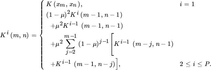
As a direct consequence of using this reproducing property, the solution is solely expressed in terms of current and previous kernel values. When a number N of training samples is available, one can explicitly compute the kernel and eventually adapt their parameters. In the more interesting online case, the previous expression will also be useful because, as we will see next, the kernel function Ki(m, n) for a particular filter instantiation can be expressed as a function only of previous kernel evaluations.
A model length can be assumed for the input samples and then mapping can be applied to vectors made up of delayed windows of the signals. Note that Ki(m, n) is not necessarily equivalent to ![]() , and hence the problem is far different from those defined in previous kernel adaptive filters. To compute this kernel, one can actually resort to applying recursion formulas in Equation 9.49 and explicitly define Ki(m, n) as a function of previously computed kernels. This methodology is next illustrated for the particular recursive model structure of the γ‐filter. In this way, not only do we attain a recursive model in feature spaces, but we also avoid applying approximate methods and pre‐images.
, and hence the problem is far different from those defined in previous kernel adaptive filters. To compute this kernel, one can actually resort to applying recursion formulas in Equation 9.49 and explicitly define Ki(m, n) as a function of previously computed kernels. This methodology is next illustrated for the particular recursive model structure of the γ‐filter. In this way, not only do we attain a recursive model in feature spaces, but we also avoid applying approximate methods and pre‐images.
9.6.2 Recursive Filters in Reproducing Kernel Hilbert Spaces
Here, we illustrate the proposed methodology for building recursive filters in the RKHS. First we review the recursive AR and MA filters in kernel feature spaces, and underline their application shortcomings. Then, noting that inclusion of short‐term memory in learning machines is essential for processing time‐varying information, we analyze the particular case of the γ‐filter (Principe et al., 1993), which provides a remarkable compromise between stability and simplicity of adaptation.
Recursive Autoregressive and Moving‐Average Filters in Reproducing Kernel Hilbert Spaces
The MA filter structure for time‐series prediction is defined as

where ![]() . Accordingly, the corresponding structure can be described explicitly in RKHS:
. Accordingly, the corresponding structure can be described explicitly in RKHS:
and given that ![]() and that we can approximately expand each vector
and that we can approximately expand each vector ![]() , we have
, we have

The AR filter structure is defined according to the following expression:
where ![]() . Accordingly, the corresponding nonlinear structure can be described by
. Accordingly, the corresponding nonlinear structure can be described by
Given that ![]() and that we can approximately expand each vector
and that we can approximately expand each vector ![]() , we have
, we have

The definition of recursive kernel ARMA filters poses challenging problems, mainly due the specification of proper parameters to ensure stability. This problem is even harder when working explicitly in RKHS, because we do not have direct access to the mapped samples. We circumvent these problems both in the linear and kernel versions by considering the γ‐filter structure next.
The Recursive γ‐Filter in Reproducing Kernel Hilbert Spaces
The standard γ‐filter is defined by


where yn is the filter output signal, xn is the filter input signal, ![]() is the signal present at the input of the ith gamma tap, n is the time index, and θf = P, and θg = μ are free parameters controlling stability and memory depth.
is the signal present at the input of the ith gamma tap, n is the time index, and θf = P, and θg = μ are free parameters controlling stability and memory depth.
A formulation of the γ‐filter is possible in the RKHS as follows. Essentially, the same recursion can be expressed in a Hilbert space:


where φ(⋅) is a nonlinear transformation in an RKHS, and ![]() is a vector in this RKHS that may not be an image of a vector of the input space; that is,
is a vector in this RKHS that may not be an image of a vector of the input space; that is, ![]() . As mentioned, this model assumes linear relations between samples in the RKHS. If this assumption is insufficient to solve the identification problem at hand, the scalar sample xn can be easily changed by vector zn = [xn, xn−1⋯xn−P]T, where P is the selected time‐embedding.
. As mentioned, this model assumes linear relations between samples in the RKHS. If this assumption is insufficient to solve the identification problem at hand, the scalar sample xn can be easily changed by vector zn = [xn, xn−1⋯xn−P]T, where P is the selected time‐embedding.
Nevertheless, the weight vectors wi of Equation 9.60 are linearly spanned by the N training vectors, ![]() . By including this expansion in Equation 9.60 and applying the kernel trick,
. By including this expansion in Equation 9.60 and applying the kernel trick, ![]() , we obtain
, we obtain
The dot products can be computed by using the kernel trick and model recursion defined in Equation 9.61 as

Arranging terms in the second case of Equation 9.63, we get

The second part still has two (interestingly nonsymmetric) dot products that are not straightforwardly computable. Nevertheless, applying recursion again in Equation 9.61, this can be rewritten as

which, in turn, can be rearranged as

Term Ki−1(m − 2, n − 1) and the dot product in the second case can be recursively computed using Equations 9.64 and 9.63. Assuming that ![]() for n < 0, we obtain the recursion
for n < 0, we obtain the recursion

and finally, the recursive kernel can be rewritten as
9.7 Online Sparsification with Kernels
The idea behind sparsification methods is to construct a sparse dictionary of bases that represent the remaining data sufficiently well. As a general rule in learning theory, it is desirable to design a network with as few processing elements as possible. Sparsity reduces the complexity in terms of computation and memory, and it usually gives better generalization ability to unseen data (Platt, 1991 ; Vapnik, 1995). In the context of kernel methods, sparsification aims to identify the bases in the kernel expansion 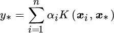 (see Equation 9.21) that can be discarded without incurring a significant performance loss.
Online sparsification is typically performed by starting with an empty dictionary, ![]() , and, in each iteration, adding the input datum xi if it fulfills a chosen sparsification criterion. We denote the dictionary at time instant n − 1 as
, and, in each iteration, adding the input datum xi if it fulfills a chosen sparsification criterion. We denote the dictionary at time instant n − 1 as ![]() , where ci is the ith stored center, taken from the input data x received up till this instant, and mn−1 is the dictionary cardinality at this instant. When a new input–output pair (xn, dn) is received, a decision is made whether or not xn should be added to the dictionary as a center. If the sparsification criterion is fulfilled, xn is added to the dictionary,
, where ci is the ith stored center, taken from the input data x received up till this instant, and mn−1 is the dictionary cardinality at this instant. When a new input–output pair (xn, dn) is received, a decision is made whether or not xn should be added to the dictionary as a center. If the sparsification criterion is fulfilled, xn is added to the dictionary, ![]() . If the criterion is not fulfilled, the dictionary is maintained,
. If the criterion is not fulfilled, the dictionary is maintained, ![]() , to preserve its sparsity.
, to preserve its sparsity.
Figure 9.7 illustrates the dictionary construction process for different sparsification approaches. Each horizontal line represents the presence of a center in the dictionary. At any given iteration, the elements in the dictionary are indicated by the horizontal lines that are present at that iteration. In the following we discuss each approach in detail.

Figure 9.7 Dictionary construction processes for different sparsification approaches. Each horizontal line marks the presence of a center in the dictionary. Top left: the ever‐growing dictionary construction, in which the dictionary contains n elements in iteration n. Top right: online sparsification by slowing down the dictionary growth, as obtained by the coherence and ALD criteria. Bottom left: sliding‐window approach, displayed with 10 elements in the dictionary. Bottom right: fixed‐budget approach, in which the pruning criterion discards one element per iteration, displayed with dictionary size 10.
9.7.1 Sparsity by Construction
We will first give a general overview of the different online sparsification methods in the literature, some of which we have already introduced in the context of the algorithms for which they were proposed. We distinguish three criteria that achieve sparsity by construction: novelty criterion, ALD criterion, and coherence criterion. If the dictionary is not allowed to grow beyond a specified maximum size, it may be necessary to discard bases at some point. This process is referred to as pruning, and we will review the most important pruning criteria later.
- Novelty criterion. The novelty criterion is a data selection method introduced by Platt (1991). It was used to construct resource‐allocating networks, which are essentially growing RBF networks. When a new data point xn is obtained by the network, the novelty criterion calculates the distance of this point to the current dictionary,
 . If this distance is smaller than some preset threshold, xn is added to the dictionary. Otherwise, it computes the prediction error, and only if this error en is larger than another preset threshold will the datum xn be accepted as a new center.
 - ALD criterion. A more sophisticated dictionary growth criterion was introduced for the KRLS algorithm in Engel et al. (2004): each time a new datum xn is observed, the ALD criterion measures how well the datum can be approximated in the feature space as a linear combination of the dictionary bases in that space. It does so by checking if the ALD condition holds; see Equation 9.43:Evaluating the ALD criterion requires quadratic complexity,

 , and therefore it is not suitable for algorithms with linear complexity such as KLMS.
 - Coherence criterion. The coherence criterion is a straightforward criterion to check whether the newly arriving datum is sufficiently informative. It was introduced in the context of the KNLMS algorithm (Richard et al., 2009). Given the dictionary Dn−1 at iteration n − 1 and the newly arriving datum xn, the coherence criterion to include the datum reads(9.66)In essence, the coherence criterion checks the similarity, as measured by the kernel function, between the new datum and the most similar dictionary center. Only if this similarity is below a certain threshold μ0 is the datum inserted into the dictionary. The higher the threshold μ0 is chosen, the more data will be accepted in the dictionary. It is an effective criterion that has linear computational complexity in each iteration: it only requires to calculate m kernel functions, making it suitable for KLMS‐type algorithms. Chen et al. (2012) introduced a similar criterion,

 , which is essentially equivalent to the coherence criterion with a Euclidean distance‐based kernel.
9.7.2 Sparsity by Pruning
In practice, it is often necessary to specify a maximum dictionary size m, or budget, that may not be exceeded; for instance, due to limitations on hardware or execution time. In order to avoid exceeding this budget, one could simply stop including any data in the dictionary once the budget is reached, hence locking the dictionary. Nevertheless, it is very probable that at some point after locking the dictionary a new datum is received that is very informative. In this case, the quality of the algorithm’s solution may improve by pruning the least relevant center of the dictionary and replacing it with the new, more informative datum.
The goal of a pruning criterion is to select a datum out of a given set, such that the algorithm’s performance is least affected. This makes pruning criteria conceptually different from the previously discussed online sparsification criteria, whose goal is to decide whether or not to include a datum. Pruning techniques have been studied in the context of NN design (Hassibi et al. 1993 ; LeCun et al. 1989) and kernel methods (De Kruif and De Vries, 2003 ; Hoegaerts et al., 2004). We briefly discuss the two most important pruning criteria that appear in kernel adaptive filtering: sliding‐window criterion and error criterion.
- Sliding window. In time‐varying environments, it may be useful to discard the oldest bases, as these were observed when the underlying model was most different from the current model. This strategy is at the core of sliding‐window algorithms such as NORMA (Kivinen et al., 2004) and SW‐KRLS (Van Vaerenbergh et al., 2006). In every iteration, these algorithms include the new datum in the dictionary and discard the oldest datum, thereby maintaining a dictionary of fixed size.
- Error criterion. Instead of simply discarding the oldest datum, the error‐based criterion determines the datum that will cause the least increase of the squared‐error performance after it is pruned. This is a more sophisticated pruning strategy that was introduced by Csató and Opper (2002) and De Kruif and De Vries (2003) and requires quadratic complexity to evaluate,
 . Interestingly, if the inverse kernel matrix is available, it is straightforward to evaluate this criterion. Given the ith element on the diagonal of the inverse kernel matrix, [K−1]ii, and the ith expansion coefficient αi, the squared error after pruning the ith center from a dictionary is αi/[K−1]ii. The error‐based pruning criterion therefore selects the index for which this quantity is minimized,(9.67)This criterion is used in the fixed‐budget algorithms FB‐KRLS (Van Vaerenbergh et al., 2010) and KRLS‐T (Van Vaerenbergh et al., 2012b). An analysis performed by Lázaro‐Gredilla et al. (2011) shows that the results obtained by this criterion are very close to the optimal approach, which is based on minimization of the KL divergence between the original and the approximate posterior distributions.
Currently, the most successful pruning criteria used in the kernel adaptive filtering literature have quadratic complexity, ![]() and therefore they can only be used in KRLS‐type algorithms. Optimal pruning in KLMS is a particularly challenging problem, as it is hard to define a pruning criterion that can be evaluated with linear computational complexity. A simple criterion is found in (Rzepka, 2012), where the center with the least weight is pruned, and weight is determined by the associated expansion coefficient,
and therefore they can only be used in KRLS‐type algorithms. Optimal pruning in KLMS is a particularly challenging problem, as it is hard to define a pruning criterion that can be evaluated with linear computational complexity. A simple criterion is found in (Rzepka, 2012), where the center with the least weight is pruned, and weight is determined by the associated expansion coefficient,
The design of more sophisticated pruning strategies is currently an open topic in KLMS literature. Some recently proposed criteria can be found in Zhao et al. (2013, 2016).
9.8 Probabilistic Approaches to Kernel Adaptive Filtering
In many signal processing applications, the problem of signal estimation is addressed. Probabilistic models have proven to be very useful in this context (Arulampalam et al. 2002 ; Rabiner 1989). One of the advantages of probabilistic approaches is that they force the designer to specify all the prior assumptions of the model, and that they make a clear separation between the model and the applied algorithm. Another benefit is that they typically provide a measure of uncertainty about the estimation. Such an uncertainty estimate is not provided by classical kernel adaptive filtering algorithms, which produce a point estimate without any further guarantees.
In this section, we will review how the probabilistic framework of GPs allows us to extend kernel adaptive filters to probabilistic methods. The resulting GP‐based algorithms not only produce an estimate of an unknown function, but also an entire probability distribution over functions; see Figure 9.8. Before we describe any probabilistic kernel adaptive filtering algorithms, it is instructive to take a step back to the nonadaptive setting, and consider the KRR problem in Equation 9.32. We will adopt the GP framework to analyze this problem from a probabilistic point of view.

Figure 9.8 Functions drawn from a GP with a squared exponential covariance K(x, x′) = exp(−∥x − x′∥2/2σ2). The 95% confidence interval is plotted as the shaded area. Up: draws from the prior function distribution. Down: draws from the posterior function distribution, which is obtained after five data points (blue crosses) are observed. The predictive mean is displayed in black.
9.8.1 Gaussian Processes and Kernel Ridge Regression
Let us assume that the observed data in a regression problem can be described by the model dn = f(xn) + ɛn, in which f represents an unobservable latent function and ![]() is zero‐mean Gaussian noise. Note that, unlike in previous chapters, here we use σ2 for the noise variance and not for the Gaussian kernel length‐scale parameter to avoid confusion with the time instant subscript n. We will furthermore assume a zero‐mean GP prior on f(x)
is zero‐mean Gaussian noise. Note that, unlike in previous chapters, here we use σ2 for the noise variance and not for the Gaussian kernel length‐scale parameter to avoid confusion with the time instant subscript n. We will furthermore assume a zero‐mean GP prior on f(x)
and a Gaussian prior on the noise ϵ, ![]() . In the GP literature, the kernel function K(x, x′) is referred to as the covariance, since it specifies the a priori relationship between values f(x) and f(x′) in terms of their respective locations, and its parameters are called hyperparameters.
. In the GP literature, the kernel function K(x, x′) is referred to as the covariance, since it specifies the a priori relationship between values f(x) and f(x′) in terms of their respective locations, and its parameters are called hyperparameters.
By definition, the marginal distribution of a GP at a finite set of points is a joint Gaussian distribution, with its mean and covariance being specified by the functions m(x) and K(x, x′) evaluated at those points (Rasmussen and Williams, 2006). Thus, the joint distribution of outputs d = [d1, …, dn]T and the corresponding latent vector ![]() is
is
By conditioning on the observed outputs y, the posterior distribution over the latent vector can be inferred
Assuming this posterior is obtained for the data up till time instant n − 1, the predictive distribution of a new output dn at location xn is computed as
The mode of the predictive distribution, given by μGP, n in Equation 9.72b, coincides with the prediction of KRR, given by Equation 9.34, showing that the regularization in KRR can be interpreted as a noise power σ2. Furthermore, the variance of the predictive distribution, given by σGP, n2 in Equation 9.72c, coincides with Equation 9.40, which is used by the ALD dictionary criterion for KRLS.
9.8.2 Online Recursive Solution for Gaussian Processes Regression
A recursive update of the complete GP in Equation 9.72 was proposed by Csató and Opper (2002), as the sparse online GP (SOGP) algorithm. We will follow the notation of Van Vaerenbergh et al. (2012b), whose solution is equivalent to SOGP but whose choice of variables allows for an easier interpretation. Specifically, the predictive mean and covariance of the GP solution in Equation 9.72 can be updated as


where Xn contains the n input data, ![]() , and
, and ![]() and
and ![]() are the predictive variances of the latent function and the new output respectively, calculated at the new input. Details can be found in Lázaro‐Gredilla et al. (2011) and Van Vaerenbergh et al. (2012b). In particular, the update of the predictive mean can be shown to be equivalent to the KRLS update. The advantage of using a full GP model is that not only does it allow us to update the predictive mean, as does KRLS, but it keeps track of the entire predictive distribution of the solution. This allows us, for instance, to establish CIs when predicting new outputs.
are the predictive variances of the latent function and the new output respectively, calculated at the new input. Details can be found in Lázaro‐Gredilla et al. (2011) and Van Vaerenbergh et al. (2012b). In particular, the update of the predictive mean can be shown to be equivalent to the KRLS update. The advantage of using a full GP model is that not only does it allow us to update the predictive mean, as does KRLS, but it keeps track of the entire predictive distribution of the solution. This allows us, for instance, to establish CIs when predicting new outputs.
Similar to KRLS, this online GP update assumes a stationary model. Interestingly, however, the Bayesian approach (and in particular its handling of the uncertainty) does allow for a principled extension that performs tracking, as we briefly discuss in what follows.
9.8.3 Kernel Recursive Least Squares Tracker
Van Vaerenbergh et al. (2012b) presented a KRLS‐T algorithm that explicitly handles uncertainty about the data, based on the probabilistic GP framework. In stationary environments it operates identically to the earlier proposed SOGP from Csató and Opper (2002), though it includes a forgetting mechanism that enables it to handle nonstationary scenarios as well. During each iteration, KRLS‐T performs a forgetting operation in which the mean and covariance are replaced through
The effect of this operation on the predictive distribution is shown in Figure 9.9. For illustration purposes, the forgetting factor is chosen unusually low, λ = 0.9.
Figure 9.9 Forgetting operation of KRLS‐T. The original predictive mean and variance are indicated as the black line and shaded gray area, as in Figure 9.8. After one forgetting step, the mean becomes the dashed red curve, and the new 95% CI is indicated in blue.
This particular form of forgetting corresponds to blending the informative posterior with a “noise” distribution that uses the same color as the prior. In other words, forgetting occurs by taking a step back toward the prior knowledge. Since the prior has zero mean, the mean is simply scaled by the square root of the forgetting factor λ. The covariance, which represents the posterior uncertainty on the data, is pulled toward the covariance of the prior. Interestingly, a regularized version of RLS (known as extended RLS) can be obtained by using a linear kernel with the B2P forgetting procedure. Standard RLS can be obtained by using a different forgetting rule; see Van Vaerenbergh et al. (2012b).
The KRLS‐T algorithm can be seen as a probabilistic extension of KRLS that obtains CIs and is capable of adapting to time‐varying environments. It obtains state‐of‐the‐art performance in several nonlinear adaptive filtering problems – see Van Vaerenbergh and Santamaría (2013) and the results of Figure 9.6 – though it has a more complex formulation than most other kernel adaptive filters and it requires a higher computational complexity. We will explore these aspects through additional examples in Section 9.10.
9.8.4 Probabilistic Kernel Least Mean Squares
The success of the probabilistic approach for KRLS‐like algorithms has led several researchers to investigate the design of probabilistic KLMS algorithms. The low complexity of KLMS‐type algorithms makes them very popular in practical solutions. Nevertheless, this low computational complexity is also a limitation that makes the design of a probabilistic KLMS algorithm a particularly hard research problem.
Some advances have already been made in this direction. Specifically, Park et al. (2014) proposed a probabilistic KLMS algorithm, though it only considered the MAP estimate. Van Vaerenbergh et al. (2016a) showed that several KLMS algorithms can be obtained by imposing a simplifying restriction on the full SOGP model, thereby linking KLMS algorithms and online GP approaches directly.
9.9 Further Reading
A myriad of different kernel adaptive filtering algorithms have appeared in the literature. We described the most prominent algorithms, which represent the state of the art. While we only focused on their online learning operation, several other aspects are worth studying. In this section, we briefly introduce the most interesting topics that are the subject of current research.
9.9.1 Selection of Kernel Parameters
As we saw in Chapter 8, hyperparameters of GP models are typically inferred by type‐II ML. This corresponds to optimal choices for KRR, due to the correspondence between GP regression and KRR, and for several kernel adaptive filters as well. A case study for KRLS and KRLS‐T can be found in Van Vaerenbergh et al. (2012a). The following should be noted, however. In online scenarios, it would be interesting to perform an online estimation of the optimal hyperparameters. This, however, is a difficult open research problem for which only a handful of methods have been proposed; see for instance Soh and Demiris (2015). In practice, it is still more appropriate to perform type‐II ML offline on a batch of training data, before running the online learning procedure using the hyperparameters found.
9.9.2 Multi‐Kernel Adaptive Filtering
In the last decade, several methods have been proposed to consider multiple kernels instead of a single one (Bach et al., 2004 ; Sonnenburg et al., 2006a). The different kernels may correspond to different notions of similarity, or they may address information coming from multiple, heterogeneous data sources. In the field of linear adaptive filtering, it was shown that a convex combination of adaptive filters can improve the convergence rate and tracking performance (Arenas‐García et al., 2006) compared with running a single adaptive filter. Multi‐kernel adaptive filtering combines ideas from the aforementioned two approaches (Yukawa, 2012). Its learning procedure activates those kernels whose hyperparameters correspond best to the currently observed data, which could be interpreted as a form of hyperparameter learning. Furthermore, the adaptive nature of these algorithms allows them to track the importance of each kernel in time‐varying scenarios, possibly giving them an advantage over single‐kernel adaptive filtering. Several multi‐kernel adaptive filtering algorithms have been proposed in the recent literature (Gao et al. e.g., 2014 ; Ishida and Tanaka e.g., 2013 ; Pokharel et al. e.g., 2013 ; Yukawa e.g., 2012). While they show promising performance gains over single‐kernel adaptive filtering algorithms, their computational complexity is much higher. This is an important aspect inherent to the combination of multiple kernel methods, and it is a topic of current research.
9.9.3 Recursive Filtering in Kernel Hilbert Spaces
Modeling and prediction of time series with kernel adaptive filters is usually addressed by time‐embedding the data, thus considering each time lag as a different input dimension. As we have already seen in previous chapters, this approach presents some important drawbacks, which become more evident in adaptive, online settings: first, the optimal filter order may change over time, which would require an additional tracking mechanism; second, if the optimal filter order is high, as for instance in audio applications (Van Vaerenbergh et al., 2016b), the method be affected by the curse of dimensionality. For some problems, the concept of an optimal filter order may not even make sense.
An alternative approach to modeling and predicting time series is to construct recursive kernel machines, which implement recursive models explicitly in the RKHS. Preliminary work in this direction considered the design of a recursive kernel in the context of infinite recurrent NNs (Hermans and Schrauwen, 2012). More recently, explicit recursive versions of the AR, MA, and gamma filters in RKHS were proposed (Tuia et al., 2014), as we have revised before. By exploiting properties of functional analysis and recursive computation, this approach avoids the reduced‐rank approximations that are required in standard kernel adaptive filters. Finally, a kernel version of the ARMA filter was presented by Li and Príncipe (2016).
9.10 Tutorials and Application Examples
This section presents experiments in which kernel adaptive filters are applied to time‐series prediction and nonlinear system identification. These experiments are implemented using code based on the KAFBOX toolbox available on the book’s web page (Van Vaerenbergh and Santamaría, 2013). Also, some examples of explicit recursivity in RKHS are provided.
9.10.1 Kernel Adaptive Filtering Toolbox
KAFBOX is a MATLAB benchmarking toolbox to evaluate and compare kernel adaptive filtering algorithms. It includes a large list of algorithms that have appeared in the literature, and additional tools for hyperparameter estimation and algorithm profiling, among others.
The kernel adaptive filtering algorithms in KAFBOX are implemented as objects using the classdef syntax. Since all KAF algorithms are online methods, each of them includes two basic operations: (1) obtaining the filter output, given a new input x*; and (2) training on a new data pair (xn, dn). These operations are implemented as the methods evaluate and train respectively.
As an example, we list the code for the KLMS algorithm in Listing 9.9. The object definition contains two sets of properties: one for the hyperparameters and one for the variables it will learn. The first method is the object’s constructor method, which copies the specified hyperparameter settings. The second method is the evaluate function, which performs the operation ![]() . It includes an
. It includes an if clause to check if the algorithm has at least performed one training step yet. If not, zeros are returned as predictions. Finally, the train method implements a single training step of the online learning algorithm. This method typically handles algorithm initialization as well, such that functions that operate on a KAF object do not have to worry about initializing. The training step itself is summarized in very few lines of MATLAB code, for many algorithms. For the following experiments, we will use v2.0 of KAFBOX.
9.10.2 Prediction of a Respiratory Motion Time Series
In the first experiment we apply KAF algorithms to predict a biomedical time series, more specifically a respiratory motion trace. These data come from robotic radiosurgery, in which a photon beam source is used to ablate tumors. The beam is operated by a robot arm that aims to move the beam source to compensate for the motion of internal organs. Traditionally, this is achieved by recording the motion of markers applied to the body surface and by using this motion to draw conclusions about the tumor position. Although this method significantly increases the targeting accuracy, the system delay arising from data processing and positioning of the beam results in a systematic error. This error can be decreased by predicting the motion of the body surface (Ernst, 2012).
The data were recorded at Georgetown University Hospital using CyberKnife® equipment, and it represents the recorded position of one of the markers attached to the body surface.3 A snapshot of this motion trace is shown in Figure 9.10. The delay to compensate totals 115 ms, which, at a sampling frequency of 26 Hz, corresponds to three samples. The task thus consists of three‐step ahead prediction. We use a time‐embedding of eight samples. Since the breathing pattern may change over time, we employed only tracking algorithms. Their parameters are listed in Table 9.1. The MSE results of the four algorithms are displayed in the last column of last column of this table. A comparison of the original series and the predictions of one of the algorithms is shown in Figure 9.11. The code to reproduce these results can be found in Listing 9.10.

Figure 9.10 A snapshot of the respiratory motion trace.
Table 9.1 Parameters used for predicting the respiratory motion trace, MSE result for three‐step ahead prediction, and measured training time.
| Algorithm | Parameters | MSE performance (dB) | Training time (s) |
| NORMA | λ = 10−4, τ = 30 | −5.78 | 0.16 |
| QKLMS | η = 0.99, |
−8.14 | 0.18 |
| SWKRLS | c = 10−4, m = 50 | −13.35 | 0.29 |
| KRLS‐T | −18.16 | 0.54 |

Figure 9.11 The respiratory motion trace and the three‐step ahead prediction of a KAF algorithm.
9.10.3 Online Regression on the KIN40K Dataset
In the second experiment we train the online algorithms to perform regression of the KIN40K dataset (Ghahramani, 1996), 4 which is a standard regression problem in the machine‐learning literature. The KIN40K data set is obtained from the forward kinematics of an eight‐link all‐revolute robot arm, similar to the one depicted in Figure 9.12. It contains 40 000 examples, each consisting of an eight‐dimensional input vector and a scalar output. KIN40K was generated with maximum nonlinearity and little noise, representing a very difficult regression test.

Figure 9.12 Sketch of a five‐link all‐revolute robot arm. The data used in the KIN40K experiment were generated by simulating an eight‐link extension of this arm.
In this experiment, we first determine the optimal hyperparameters for the kernel adaptive filters by running the tool kafbox_parameter_estimation, which is based on the GPML toolbox from Rasmussen and Williams (2006). We use 1000 randomly selected data points for the hyperparameter optimization. In the literature, an anisotropic kernel function, which has a different kernel width per dimension, is commonly used on these data. For simplicity, though, we employ an isotropic Gaussian kernel. The hyperparameters found by the optimization procedure are listed in Table 9.2. The forgetting factor is only used by KRLS‐T, though its optimal value is determined to be 1, which indicates that no forgetting takes place in practice.
Table 9.2 Optimal hyperparameters found for the KIN40K regression problem.
| Parameter | Optimal value |
| Kernel width σ | 1.66 |
| Regularization | 2.47 × 10⁻⁶ |
| Forgetting factor λ | 1 |
From the remaining data we randomly select 5000 data points for training and 5000 data for testing the regression. Apart from the hyperparameters that are determined automatically in this experiment, the kernel adaptive filters have some parameters relating to memory size and learning rate. The values chosen for these parameters are listed in Table 9.3. The values for QKLMS are chosen such that it obtains optimal performance after training with a dictionary size that is one order of magnitude larger than that of the KRLS algorithms. The precision parameter ν of KRLS is tuned to yield a dictionary size of around m = 500 at the end of the experiment, which is the budget of SWKRLS and KRLS‐T. The learning curves for this experiment are shown in Figure 9.13. The code for reproducing this experiment is available on the book’s web page and in the KAFBOX toolbox demos.
Table 9.3 Additional parameters used in the KIN40K regression experiment, final dictionary size, and measured training time.
| Algorithm | Parameters | Final dictionary size | Training time (s) |
| QKLMS | η = 0.99, |
2750 | 18.51 |
| KRLS | ν = 0.32 | 510 | 12.09 |
| FBKRLS | m = 500 | 500 | 33.49 |
| KRLS‐T | m = 500 | 500 | 86.41 |

Figure 9.13 Learning curves of different algorithms on the KIN40K data.
9.10.4 The Mackey–Glass Time Series
The Mackey–Glass time‐series prediction is a benchmarking problem in nonlinear time‐series modeling. We discussed this time series and the prediction results for KLMS and KRLS in Sections 9.4.3 and 9.5.3 respectively. The learning curves, shown in Figure 9.4, indicate that KLMS converges very slowly, and that KRLS can obtain a much lower MSE in less iterations. On the other hand, KRLS requires an order of magnitude more computation and memory. These results are in line with the intuitions from linear adaptive filtering, in which LMS and RLS represent two different choices in the compromise between complexity and convergence rate. Nevertheless, there is a fundamental difference between the complexity analysis of linear and kernel adaptive filtering algorithms. While in linear adaptive filters the complexity depends on the data dimension, in KAF algorithms it depends on the dictionary size. And, importantly, the latter is a parameter that can be controlled.
A KRLS‐type algorithm with a large dictionary can converge faster than a KLMS‐type algorithm with a similarly sized dictionary, at the expense of a higher computational complexity. But it would be instructive to ask how a KRLS‐type algorithm with a small dictionary compares with a KLMS‐type algorithm with a large dictionary. Can the KRLS algorithm obtain similar complexity as KLMS, while maintaining its better convergence rate? This question is answered in the diagrams of Figure 9.14. We have included two KAF algorithms, QKLMS and KRLS‐T, that allow easy control over their dictionary size.

Figure 9.14 MSE versus complexity trade‐off comparisons for prediction of the Mackey–Glass time series. Up: maximum number of floating point operations (FLOPS) per iteration as a function of the steady‐state MSE. Down: maximum number of bytes per iteration as a function of the steady‐state MSE. Each marker represents a single run of one of the algorithms with a single set of parameters. The start of each parameter sweep is indicated by a black dot.
Figure 9.14 presents the results obtained by the KAF profiler tool included in KAFBOX. The MATLAB code to reproduce this figure is available on the book’s web page. The profiler tool runs each algorithm several times with different configurations, whose parameters are shown in Table 9.4, producing one point in the plot per algorithm configuration. It calculates several variables, such as the number of FLOPS, the memory (in bytes) used, and execution time.
Table 9.4 Parameters used in the Mackey–Glass time‐series prediction. A Gaussian kernel with σ = 1 was used.
| Algorithm | Fixed parameters | Varying parameter |
| QKLMS | η = 0.5 | |
| KRLS‐T | λ = 1, |
m ∈{3, 5, 7, 10, 20, 30, 50, 150} |
By plotting the MSE versus the FLOPS or memory, we get an idea of the resources required to obtain a desired MSE result. If, for instance, we are working in a scenario with a restriction on computational complexity, we should select the algorithm that performs best under this restriction by determining which performance curve is most to the left for the amount of FLOPS available. In the same manner, by fixing a maximum on MSE we obtain the FLOPS and memory required by each algorithm. In the left plot of Figure 9.14 we observe that if the available computational complexity is very limited, it may be more interesting to use QKLMS. In other cases, KRLS‐T is preferred as a better MSE is obtained for the same amount of FLOPS. In terms of memory used, it appears that it is always advantageous to use KRLS‐T, as can be seen in the right plot.
9.10.5 Explicit Recursivity on Reproducing Kernel in Hilbert Space and Electroencephalogram Prediction
This experiment deals with a real EEG signal prediction problem with four‐samples ahead. This is a very challenging nonlinear problem with high levels of noise and uncertainty. We used file “SLP01A” from the MIT‐BIH Polysomnographic Database.5 All recordings in the database include an ECG signal, an invasive blood pressure signal, an EEG signal, and a respiration signal. In this experiment, we considered the prediction of the EEG signal. As for the MG experiments, we used {50, 100, 200} training samples, while the next 2000 samples were used for prediction. Listing 9.11 gives a simple piece of code for the implementation of the recursive kernel γ‐filter, which can be used to generate the appropriate code for obtaining the results.
Figure 9.15 shows the KRR prediction of two different EEG segments in the test set for the different approaches; all the methods show the tendency to oversmooth data where peaks are observed. Nonetheless, the K2 kernel always outperforms the other approaches, confirming the numerical results.

Figure 9.15 Predictions in two different EEG segments for the recursive Kc, the standard KRR K2, and the lagged Kl kernels.
9.10.6 Adaptive Antenna Array Processing
This last real example illustrates the method in a purely adaptive setting of high complexity. The problem deals with array processing using a planar antenna array model that consists of 3 × 3 circular printed patches tuned at a frequency of 1.87 GHz. The distance between patches has been set to 0.5λ. The chosen substrate was PVC. We computed the excitation voltage Vn of each element for five different angles of arrival. In order to compute these excitations, we assume that ![]() , where
, where ![]() is the ideal excitation, and
is the ideal excitation, and ![]() is the one produced by the mutual coupling between antenna elements (Pozar, 2003). We run five finite‐difference time‐domain‐based simulations using CST Microwave Studio 2008 (http://www.cst.com) to obtain the active reflection coefficients Γn, and then the excitation voltages Vn produced by each angle of arrival. The azimuth and elevation angles of arrival were 0°, − 20°, 20°, 30° and − 135° and 0°, − 5°, 5°, − 5° and − 20° degrees respectively.
is the one produced by the mutual coupling between antenna elements (Pozar, 2003). We run five finite‐difference time‐domain‐based simulations using CST Microwave Studio 2008 (http://www.cst.com) to obtain the active reflection coefficients Γn, and then the excitation voltages Vn produced by each angle of arrival. The azimuth and elevation angles of arrival were 0°, − 20°, 20°, 30° and − 135° and 0°, − 5°, 5°, − 5° and − 20° degrees respectively.
Transmitted signals consisted of frames containing 142 binary phase‐shift keying symbols, of which the 26 central ones (midamble) are training samples, and the rest contain the transmitted information. Users are assumed to transmit frames synchronously. In the simulated scenario, 10 realizations contained 200 frames. At the beginning of each simulation, the five users transmitted independent signals with equal power P. At frame 66, users 3 and 5 switch off and users 1, 2, and 4 change their power to 0.64P. At frame 131, user 3 switches on and all users transmit at power P. The SNR with respect to user 4 (taken as the desired one) was 10 dB all times.
Figure 9.16 illustrates the BER as a function of time for the desired user. We compare our method (RKHS–KRLS) with the KLMS (Liu et al., 2008), KRLS (Engel et al., 2004), along with their sparse versions via “surprise criterion” (Liu et al., 2009) using the standard RBF kernel. The regularization factor was set to η = 0.001, the forgetting factor to 0.99, and the threshold used in approximate linear dependency was set to 0.55. The recursive kernel used μ = 0.9. The experiment was repeated 10 times and the average curves are shown. The recursive kernel has the same computational as embedding‐based kernels (Table 9.5). The optimization computational time of the recursive kernel algorithm is ![]() , which is the same as KRLS. The added computational burden comes from the computation of the kernels. Both algorithms need to compute a vector of kernel products per iteration. The recursive kernel needs an additional computational time of
, which is the same as KRLS. The added computational burden comes from the computation of the kernels. Both algorithms need to compute a vector of kernel products per iteration. The recursive kernel needs an additional computational time of ![]() to implement the recursion of Equation 9.65. A higher memory space is needed because the P kernel matrices of the recursion plus their combination need to be stored. Following Equation 9.65, kernel entries depend solely on previous kernels. In addition, the information introduced by each sample into the first kernel (P = 1) propagates through the following kernels in subsequent recursion steps with a decaying factor depending on 1 − μ. Also, the recursive kernel yields, in general, lower error bounds in steady state and shows competitive performance with KRLS when the channel changes. The method is implemented here using only scalars, and hence it shows a slightly longer convergence time than the rest of the methods. Extension of the method to considering deeper embeddings is straightforward and will be studied in the future. The recursive kernel used in this example is available on the book’s web page.
to implement the recursion of Equation 9.65. A higher memory space is needed because the P kernel matrices of the recursion plus their combination need to be stored. Following Equation 9.65, kernel entries depend solely on previous kernels. In addition, the information introduced by each sample into the first kernel (P = 1) propagates through the following kernels in subsequent recursion steps with a decaying factor depending on 1 − μ. Also, the recursive kernel yields, in general, lower error bounds in steady state and shows competitive performance with KRLS when the channel changes. The method is implemented here using only scalars, and hence it shows a slightly longer convergence time than the rest of the methods. Extension of the method to considering deeper embeddings is straightforward and will be studied in the future. The recursive kernel used in this example is available on the book’s web page.
Figure 9.16 BER as a function of time (training frames) for the desired user.
Table 9.5 Computational complexity at iteration t.
| Algorithm | LMS | KLMS | KRLS | Proposed RKHS recursivity |
| Computation | ||||
| Memory |
9.11 Questions and Problems
- Exercise 9.11.1 Discuss when it is more useful to use a KLMS‐like algorithm and when a KRLS‐like algorithm.
- Exercise 9.11.2 Demonstrate that the computational complexity of KLMS is
 , where m is the number of data in its dictionary.
 - Exercise 9.11.3 Demonstrate that the computational complexity of KRLS is
 , where m is the number of data in its dictionary.
 - Exercise 9.11.4 List the advantages and disadvantages of using a sliding‐window approach for determining a filter dictionary, as used for instance by SW‐KRLS and NORMA.
- Exercise 9.11.5 Demonstrate that the recursive kernel gamma filter is unique and bounded.
- Exercise 9.11.6 In the tracking experiment of Section 9.5.5, the slope of the learning curve for some algorithms is less steep just after the switch than at the beginning of the experiment. Identify for which algorithms this happens, in Figure 9.6, and explain for each of these algorithms why this is the case.