
12
Kernel Feature Extraction in Signal Processing
Kernel‐based feature extraction and dimensionality reduction are becoming increasingly important in advanced signal processing. This is particularly relevant in applications dealing with very high‐dimensional data. Current methods tackle important problems in signal processing: from signal subspace identification to nonlinear blind source separation, as well as nonlinear transformations that maximize particular criteria, such as variance (KPCA), covariance (kernel PLS (KPLS)), MSE (kernel orthonormalized PLS (KOPLS)), correlation (kernel canonical correlation analysis (KCCA)), mutual information (kernel generalized variance) or SNR (kernel SNR), just to name a few. Kernel multivariate analysis (KMVA) has closed links to KFD analysis as well as interesting relations to information theoretic learning. The application of the methods is hampered in two extreme cases: when few examples are available the extracted features are either overfitted or meaningless, while in large‐scale settings the computational cost is prohibitive. Semi‐supervised and sparse learning have entered the field to alleviate these problems. Another field of intense activity is that of domain adaptation and manifold alignment, for which kernel method feature extraction is currently being used. All these topics are the subject of this chapter. We will review the main kernel feature extraction and dimensionality reduction methods, dealing with supervised, unsupervised and semi‐supervised settings. Methods will be illustrated in toy examples, as well as real datasets.
12.1 Introduction
In the last decade, the amount and diversity of sensory data has increased vastly. Sensors and systems acquire signals at higher rate and resolutions, and very often data from different sensors need to be combined. In this scenario, appropriate data representation, adaptation, and dimensionality reduction become important concepts to be considered. Among the most important tasks of machine learning are feature extraction and dimensionality reduction, mainly due to the fact that, in many fields, practitioners need to manage data with a large dimensionality; for example, in image analysis, medical imaging, spectroscopy, or remote sensing, and where many heterogeneous feature components are computed from data and grouped together for machine‐learning tasks.
Extraction of relevant features for the task at hand boils down to finding a proper representation domain of the problem. Different objectives will give different optimization problems. The field dates back to the early 20th century with the works of Hotelling, Wold, Pearson, and Fisher, just to name a few.1 They originated the field of multivariate analysis (MVA) in its own right. The methods developed for MVA address the problems of dimensionality reduction in a very principled way, and typically resort to linear algebra operations. Owing to their simplicity and uniqueness of the solution, MVA methods have been successfully used in several scientific areas (Wold, 1966a).
Roughly speaking, the goal of MVA methods is to exploit dependencies among the variables to find a reduced set of them that are relevant for the learning task. PCA, PLS, or CCA are amongst the best known MVA methods. PCA uses only the correlation between the input dimensions in order to maximize the variance of the data over a chosen subspace, disregarding the target data. PLS and CCA choose subspaces where the projections maximize the covariance and the correlation between the features and the targets, respectively. Therefore, they should in principle be preferred to PCA for regression or classification problems. In this chapter, we consider also a fourth MVA method known as OPLS that is also well suited to supervised problems, with certain optimality in LS multiregression.
In any case, all these MVA methods are constrained to model linear relationships between the input and output; thus, they will be suboptimal when these relationships are actually nonlinear. This issue has been addressed by constructing nonlinear versions of MVA methods. They can be classified into two fundamentally different approaches (Rosipal, 2011): (1) the modified methods in which the linear relations among the latent variables are substituted by nonlinear relations (Laparra et al. 2014, 2015; Qin and McAvoy 1992; Wold et al. 1989); and (2) variants in which the algorithms are reformulated to fit a kernel‐based approach (Boser et al. 1992; Schölkopf et al. 1998; Shawe‐Taylor and Cristianini 2004). An appealing property of the resulting kernel algorithms is that they obtain the flexibility of nonlinear expressions using straightforward methods from linear algebra.
The field has captured the attention of many researchers from other fields mainly due to interesting relations to KFD analysis algorithms (a plethora of variants has been introduced in the last decade in the fields of pattern recognition and computer vision), and the more appealing relations to particular instantiations of kernel methods for information theoretic learning (e.g., links between covariance operators in Hilbert spaces and information concepts such as mutual information or Rényi entropy). In Section 12.3 we will show some of the relations between KMVA and other feature extraction methods based on nonparametric kernel dependence estimates.
The fact that KMVA methods need the construction of a Gram matrix of kernel dot products between data precludes their direct use in applications involving large datasets, and the fact that in many applications only a small number of labeled samples is also strongly limiting. The first difficulty is usually minimized by the use of sparse or incremental versions of the algorithms, and the second has been overcome by the field of SSL. Approaches to tackle these problems include special types of regularization, guided either by selection of a reduced number of basis functions or by considering the information about the manifold conveyed by the unlabeled samples. This chapter reviews all these approaches (Section 12.4).
Domain adaptation, transfer learning, and manifold alignment are relevant topics nowadays. Note that classification or regression algorithms developed with data coming from one domain (system, source) cannot be directly used in another related domain, and hence adaptation of either the data representation or the classifier becomes strictly imperative (Quiñonero‐Candela et al., 2009; Sugiyama and Kawanabe, 2012). The fields of manifold alignment and domain adaptation have captured high interest nowadays in pattern analysis and machine learning. On many occasions, it is more convenient to adapt the data representations to facilitate the use of standard classifiers, and several kernel methods have been proposed trying to map different data sources to a common latent space where the different source manifolds are matched. Section 12.5 reviews some kernel methods to perform domain adaptation while still using linear algebra.
12.2 Multivariate Analysis in Reproducing Kernel Hilbert Spaces
This section fixes the notation used in the chapter, and reviews the framework of MVA both in the linear case and with kernel methods. An experimental evaluation on standard UCI datasets and real high‐dimensional image segmentation problems illustrate the performance of all the methods.
12.2.1 Problem Statement and Notation
Assume any supervised regression or classification problem, were X and Y are column‐wise centered input and target data matrices of sizes N × d and N × m respectively. Here, N is the number of training data points in the problem, and d and m are the dimensions of the input and output spaces respectively. The output response data (sometimes referred to as the target) Y are typically a set of variables in columns that need to be approximated in regression settings, or a matrix that encodes the class membership information in classification settings. The sample covariance matrices are given by Cx = (1/N)XTX and Cy = (1/N)YTY, whereas the input–output cross‐covariance is expressed as Cxy = (1/N)XTY.
The objective of standard linear multiregression is to adjust a linear model for predicting the output variables from the input ones; that is, ![]() , where W contains the regression model coefficients. The standard LS solution is W = X†Y, where X† = (XTX)−1XT is the Moore–Penrose pseudoinverse2 of X. If some input variables are highly correlated, the corresponding covariance matrix will be rank deficient, and thus its inverse will not exist. The same situation will be encountered if the number N of data is less that the dimension d of the space. In order to turn these problems into well‐conditioned ones it is usual to apply a Tikhonov regularization term; for instance, by also minimizing the Frobenius norm of the weights matrix
, where W contains the regression model coefficients. The standard LS solution is W = X†Y, where X† = (XTX)−1XT is the Moore–Penrose pseudoinverse2 of X. If some input variables are highly correlated, the corresponding covariance matrix will be rank deficient, and thus its inverse will not exist. The same situation will be encountered if the number N of data is less that the dimension d of the space. In order to turn these problems into well‐conditioned ones it is usual to apply a Tikhonov regularization term; for instance, by also minimizing the Frobenius norm of the weights matrix ![]() one obtains the regularized LS solution W = (XTX + λI)−1XTY, where parameter λ controls the amount of regularization.
one obtains the regularized LS solution W = (XTX + λI)−1XTY, where parameter λ controls the amount of regularization.
MVA techniques solve the aforementioned problems by projecting the input data into a subspace that preserves the information useful for the current machine‐learning problem. MVA methods transform the data into a set of features through a transformation X′ = XU, where ![]() will be referred hereafter as the projection matrix, ui being the ith projection vector and nf the number of extracted features. Some MVA methods consider also a feature extraction in the output space, Y′ = YV, with
will be referred hereafter as the projection matrix, ui being the ith projection vector and nf the number of extracted features. Some MVA methods consider also a feature extraction in the output space, Y′ = YV, with ![]() .
.
Generally speaking, MVA methods look for projections of the input data that are “maximally aligned” with the targets. Different methods are characterized by the specific objectives they maximize. Table 12.1 summarizes the MVA methods that are being presented in this section. It is important to be aware of that MVA methods are based on the first‐ and second‐order moments of the data, so these methods can be formulated as a generalized eigenvalue problem; hence, they can be solved using standard algebraic techniques.
Table 12.1 Summary of linear and KMVA methods. We state for all methods treated in this section the objective to maximize, constraints for the optimization, and maximum number of features np that can be extracted, and how the data are projected onto the extracted features.
| Method | PCA | SNR | PLS | CCA | OPLS |
| maxu | uTCxu | uTCxyv | uTCxyv | ||
| s.t. | UTU = I | UTCnU = I |  |
 |
UTCxU = I |
| np | r(X) | r(X) | r(X) | r(Cxy) | r(Cxy) |
| P(X*) | X*U | X*U | X*U | X*U | X*U |
| KPCA | KSNR | KPLS | KCCA | KOPLS | |
| maxα | αTKxYv | αTKxYv | αTKxYYTKxα | ||
| s.t. | ATKxA = I | ATKxnKnxA = I |  |
 |
|
| np | r(Kx) | r(Kx) | r(Kx) | r(KxY) | r(KxY) |
| P |
Kx(X*, X)A | Kx(X*, X)A | Kx(X*, X)A | Kx(X*, X)A | Kx(X*, X)A |
Vectors u and α are column vectors in matrices U and A respectively. r(⋅) denotes the rank of a matrix.
12.2.2 Linear Multivariate Analysis
The best known MVA method, and probably the oldest one, is PCA (e.g., Pearson, 1901), also known as the Hotelling transform or the Karhunen–Loève transform (Jolliffe, 1986). PCA selects the maximum variance projections of the input data, imposing an orthonormality constraint for the projection vectors (see Table 12.1). This method assumes that the projections that contain the information are the ones that have the highest variance. PCA is an unsupervised feature extraction method. Even if supervised methods, which include the target information, may be preferred, PCA and its kernel version, KPCA, are used as preprocessing stages in many supervised problems, possibly because of their simplicity and ability to discard irrelevant directions (Abrahamsen and Hansen 2011; Braun et al. 2008).
In signal processing applications, maximizing the variance of the signal may not be a good idea per se, and one typically looks for transformations of the observed signal such that the SNR is maximized, or alternatively for transformations that minimize the fraction of noise. This is the case of the MNF transform (Green et al., 1998), which extends PCA by maximizing the signal variance while minimizing the estimated noise variance. Let us assume that observations xi follow an additive noise model; that is, xi = si + ni, where ni may not necessarily be Gaussian. The observed data matrix is assumed to be the sum of a “signal” and a “noise” matrix, X = s + N, being typically N > d. Matrix ![]() indicates the centered version of X, and
indicates the centered version of X, and ![]() represents the empirical covariance matrix of the input data. Very often, signal and noise are assumed to be orthogonal, sTN = NTs = 0, which is very convenient for SNR maximization and blind‐source separation problems (Green et al., 1998; Hundley et al., 2002). Under this assumption, one can incorporate easily the information about the noise through the noise covariance matrix
represents the empirical covariance matrix of the input data. Very often, signal and noise are assumed to be orthogonal, sTN = NTs = 0, which is very convenient for SNR maximization and blind‐source separation problems (Green et al., 1998; Hundley et al., 2002). Under this assumption, one can incorporate easily the information about the noise through the noise covariance matrix ![]() .
.
The PLS algorithm (Wold, 1966b) is a supervised method based on latent variables that account for the information in the cross‐covariance matrix Cxy. The strategy here consists of constructing the projections that maximize the covariance between the projections of the input and the output, while keeping certain orthonormality constraints. The procedure is solved iteratively or in block through an eigenvalue problem. In iterative schemes, datasets X and Y are recursively transformed in a process which subtracts the information contained in the already estimated latent variables. This process is usually called deflation, and it can be done in several ways that define the many variants of PLS existing in the literature.3 The algorithm does not involve matrix inversion, and it is robust against highly correlated data. These properties made it usable in many fields, such as chemometrics and remote sensing, where signals typically are acquired in a range of highly correlated spectral wavelengths.
The main feature of CCA is that it maximizes the correlation between projected input and output data (Hotelling, 1936). This is why CCA can manage spatial dimensions in the input or output data that show high variance but low correlation between input and output, which would be emphasized by PLS. CCA is a standard method for aligning data sources, with interesting relations to information‐theoretic approaches. We will come back to this issue in Sections 12.3 and 12.5.
An interesting method we will pay attention to is OPLS, also known as multilinear regression (Borga et al., 1997) or semi‐penalized CCA (Barker and Rayens, 2003). OPLS is optimal for performing multilinear LS regression on the features extracted from the training data; that is:
with W = X′†Y being the matrix containing the optimal regression coefficients. It can be shown that this optimization problem is equivalent to the one stated in Table 12.1. This problem can be compared with maximizing a Rayleigh coefficient that takes into account the projections of input and output data,  . This is why the method is called semi‐penalized CCA. Indeed, it does not take into account the variance of the projected input data, but emphasizes those input dimensions that better predict large variance projections of the target data. This asymmetry makes sense in supervised subspace learning where matrix Y contains target values to be approximated from the extracted input features.
Actually, OPLS (for classification problems) is equivalent to LDA provided an appropriate labeling scheme is used for Y (Barker and Rayens, 2003). However, in “two‐view learning” problems (also known as domain adaptation or manifold alignment), in which X and Y represent different views of the data (Shawe‐Taylor and Cristianini, 2004, Section 6.5), one would like to extract features that can predict both data representations simultaneously, and CCA could be preferred to OPLS. We will further discuss this matter in Section 12.5.
Now we can establish a simple common framework for PCA, SNR, PLS, CCA, and OPLS, following the formalization introduced in Borga et al. (1997), where it was shown that these methods can be reformulated as (generalized) eigenvalue problems, so that linear algebra packages4 can be used to solve them. Concretely:

Note that CCA and OPLS require the inversion of matrices Cx and Cy. Whenever these are rank deficient, it becomes necessary to first extract the dimensions with nonzero variance using PCA, and then solve the CCA or OPLS problems. Alternative approaches include adding extra regularization terms. A very common approach is to solve the aforementioned problems using a two‐step iterative procedure: first, the projection vectors corresponding to the largest (generalized) eigenvalue are chosen, for which there exist efficient methods such as the power method; and then in the second step known as deflation, one removes from the data (or the covariance matrices) the covariance that can be already obtained from the features extracted in the first step. Equivalent solutions can be found by formulating them as regularized LS problems. As an example, sparse versions of PCA, CCA, and OPLS were introduced by adding sparsity promotion terms, such as LASSO or ℓ1‐norm on the projection vectors, to the LS functional (Hardoon and Shawe‐Taylor 2011; Van Gerven et al. 2012; Zou et al. 2006).
12.2.3 Kernel Multivariate Analysis
The framework of KMVA algorithms is aimed at extracting nonlinear projections while actually working with linear algebra. Let us first consider a function ![]() that maps input data into a Hilbert feature space
that maps input data into a Hilbert feature space ![]() . The new mapped dataset is defined as Φ = [Φ(x1)|⋯|Φ(xl)]T, and the features extracted from the input data will now be given by Φ′ = ΦU, where matrix U is of size
. The new mapped dataset is defined as Φ = [Φ(x1)|⋯|Φ(xl)]T, and the features extracted from the input data will now be given by Φ′ = ΦU, where matrix U is of size ![]() . The direct application of this idea suffers from serious practical limitations when the
. The direct application of this idea suffers from serious practical limitations when the ![]() is very large. To implement practical KMVA algorithms we need to rewrite the equations in the first half of Table 12.1 in terms of inner products in
is very large. To implement practical KMVA algorithms we need to rewrite the equations in the first half of Table 12.1 in terms of inner products in ![]() only. For doing so, we rely on the availability of a kernel matrix Kx = ΦΦT of dimension N × N, and on the representer theorem (Kimeldorf and Wahba, 1971), which states that the projection vectors can be written as a linear combination of the training samples; that is, U = ΦTA, matrix
only. For doing so, we rely on the availability of a kernel matrix Kx = ΦΦT of dimension N × N, and on the representer theorem (Kimeldorf and Wahba, 1971), which states that the projection vectors can be written as a linear combination of the training samples; that is, U = ΦTA, matrix ![]() being the new argument for the optimization.5 Equipped with the kernel trick, one readily develops kernel versions of the previous linear MVA, as shown in Table 12.1.
being the new argument for the optimization.5 Equipped with the kernel trick, one readily develops kernel versions of the previous linear MVA, as shown in Table 12.1.
For PCA, it was Schölkopf et al. (1998) who introduced a kernel version denoted KPCA. Lai and Fyfe in 2000 first introduced the kernel version of CCA denoted KCCA (Lai and Fyfe, 2000a; Shawe‐Taylor and Cristianini, 2004). Later, Rosipal and Trejo (2001) presented a nonlinear kernel variant of PLS. In that paper, Kx and the Y matrix are deflated the same way, which is more in line with the PLS2 variant than with the traditional algorithm “PLS Mode A,” and therefore we will denote it as KPLS2. A kernel variant of OPLS was presented in (Arenas‐García et al., 2007) and is here referred to as KOPLS. Recently, the kernel MNF was introduced in (Nielsen, 2011) but required the estimation of the noise signal in input space. This kernel SNR method was extended in (Gómez‐Chova et al., 2017) to deal with signal and noise relations in Hilbert space explicitly. That is, in the explicit KSNR (KSNRe) the noise is estimated in Hilbert spaces rather than in the input space and then mapped with an appropriate reproducing kernel function (which we refer to as implicit KSNR, KSNRi).
As for the linear case, KMVA methods can be implemented as (generalized) eigenvalue problems:

Note that the output data could also be mapped to some feature space ![]() , as was considered for KCCA for a multiview learning case (Lai and Fyfe, 2000a). Here, we consider instead that it is the actual labels in Y which need to be well represented by the extracted input features, so we will deal with the original representation of the output data.
, as was considered for KCCA for a multiview learning case (Lai and Fyfe, 2000a). Here, we consider instead that it is the actual labels in Y which need to be well represented by the extracted input features, so we will deal with the original representation of the output data.
12.2.4 Multivariate Analysis Experiments
In this section we illustrate through different application examples the use and capabilities of the kernel multivariate feature extraction framework. We start with a toy example where we can visualize the features, and therefore get intuition about what is doing each method. After that we compare the performance of linear and KMVA methods in a real classification problem of (high‐dimensional) satellite images (Arenas‐García and Camps‐Valls 2008; Arenas‐García et al. 2013).
Toy Example
In this first experiment we illustrate the methods presented using toy data. Figure 12.1 illustrates the features extracted by the methods for a toy classification problem with three classes. Figure 12.1 can be reproduced by downloading the SIMFEAT toolbox and executing the script Demo_Fig_14_1.m from the book’s repository. A simplified version of the code is shown in Listing 12.1. Note how all the methods are based on eigendecompositions of covariance matrices or kernels.

Figure 12.1 Toy example of MVA methods in a three‐class problem. Top: features extracted using the training set. Figure shows the variance (var), MSE when the projection is used to approximate y, and the largest covariance (cov) and correlation (corr) achievable using a linear projection of the target data. The first thing we see is that linear methods (top row) perform a rotation on the original data, while the features extracted by the nonlinear methods (second row) are based on more complicated transforms. There is a clear difference between the unsupervised methods (PCA and KPCA) and the supervised methods, which try to pull apart the data coming from different classes. Bottom: classification of test data using a linear classifier trained in the transformed domain, numerical performance is given by the overall accuracy (OA). Since in this case there is no dimensionality reduction, all the linear methods obtain the same accuracy. However, the nonlinear methods obtain very different results. In general, nonlinear methods obtain better results than the linear ones. A special case is KPCA, which obtains very poor results. KPCA is unsupervised and in this case looking for high‐variance dimensions is not useful in order to discern between the classes. KPLS obtains lower accuracy than KOPLS and KCCA, which in turn obtain a similar result since their formulation is almost equivalent (only an extra normalization step is performed by KCCA).
The data were generated from three noisy parabolas, so that a certain overlap exists between classes. For the first extracted feature we show its sample variance, the largest correlation and covariance that can be achieved with a linear transformation of the output, and the optimum MSE of the feature when used to approximate the target. All these are shown above the scatter plot. The first projection for each method maximizes the variance (PCA), covariance (PLS), and correlation (CCA), while OPLS finds the MMSE projection. However, since these methods can just perform linear transformations of the data, they are not able to capture any nonlinear relations between the input variables. For illustrative purposes, we have included in Figure 12.1 the projections obtained using KMVA methods with an RBF kernel. Input data were normalized to zero mean and unit variance, and the kernel width σ was selected as the median of all pairwise distances between samples (Blaschko et al., 2011). The same σ has been used for all methods, so that features are extracted from the same mapping of the input data. We can see that the nonlinear mapping improves class separability.
Satellite Image Classification
Nowadays, multi‐ and hyperspectral sensors mounted on satellite and airborne platforms may acquire the reflected energy by the Earth with high spatial detail and in several spectral wavelengths. Here, we pay attention to the performance of several KMVA methods for image segmentation of hyperspectral images (Arenas‐García and Petersen, 2009). The input data X is the spectral radiance obtained for each pixel (sample) of dimension d equal to the number of spectral channels considered, and the output target variable Y corresponds to the class label of each particular pixel.
The data used is the standard AVIRIS image obtained from NW Indiana’s Indian Pine test site in June 1992.6 The 20 noisy bands corresponding to the region of water absorption have been removed, and we used pixels of dimension d = 200 spectral bands. The high number of narrow spectral bands induces a high collinearity among features. Discriminating among the major crop classes in the area can be very difficult. The image is 145 × 145 pixels and contains 16 quite unbalanced classes (ranging from 20 to 2468 pixels each). Among the available N = 10 366 labeled pixels, 20% were used to train the feature extractors, where the remaining 80% were used to test the methods. The discriminative properties of the extracted features were assessed using a simple classifier constructed with a linear model adjusted with LS plus a “winner takes all” activation function.
The result of the classification accuracy during the test for different number nf of extracted features is shown in Figure 12.2. For linear models, OPLS performs better than all other methods for any number of extracted features. Even though CCA provides similar results for nf = 10, it involves a slightly more complex generalized eigenproblem. When the maximum number of projections is used, all methods result in the same error. Nevertheless, while PCA and PLS2 require nf = 200 features (i.e., the dimensionality of the input space), CCA and OPLS only need nf = 15 features to achieve virtually the same performance.

Figure 12.2 Average classification accuracy (percent) for linear and KMVA methods as a function of the number of extracted features, along some classification maps for the case of nf = 10 extracted features.
We also considered nonlinear KPCA, KPLS2, KOPLS, and KCCA, using an RBF kernel. The width parameter of the kernel was adjusted with a fivefold cross‐validation over the training set. The same conclusions obtained for the linear case apply also to MVA methods in kernel feature space. The features extracted by KOPLS allow us to achieve a slightly better overall accuracy than KCCA, and both methods perform significantly better than KPLS2 and KPCA. In the limit of nf, all methods achieve similar accuracy. The classification maps obtained for nf = 10 confirm these conclusions: higher accuracies lead to smoother maps and smaller error in large spatially homogeneous vegetation covers.
Finally, we transformed all the 200 original bands into a lower dimensional space of 18 features and assessed the quality of the extracted features by standard PCA, SNR/MNF, KPCA, and KSNR approaches. Figure 12.3 shows the extracted features in descending order of relevance. In this unsupervised setting it is evident that incorporating the signal‐to‐noise relations in the extraction with KSNR provides some clear advantages in the form of more “noise‐free” features than the other methods.

Figure 12.3 Extracted features from the original image by PCA, MNF/SNR, KPCA, standard (implicit) KSNR, and explicit KSNR in the kernel space for the first nf = 18 components, plotted in RGB composite of three top components ordered in descending importance (images converted to grey scale for the book).
12.3 Feature Extraction with Kernel Dependence Estimates
In this section we review the connections of feature extraction when using dependency estimation as optimization criterion. First, we present a popular method for dependency estimation based on kernels, the HSIC (Gretton et al., 2005c). We will analyze the connections between HSIC and classical feature extraction methods. After that, we will review two methods that employ HSIC as optimization criterion to find interesting features: the Hilbert–Schmidt component analysis (HSCA) (Daniušis and Vaitkus, 2009) and the kernel dimensionality reduction (KDR) (Fukumizu et al. 2003, 2004). A related problem found in DSP is the BSS problem; here, one aims to find a transformation that separates the input observed signal into a set of independent signal components. We will review different BSS methods based on kernels.
12.3.1 Feature Extraction Using Hilbert–Schmidt Independence Criterion
MVA methods optimize different criteria mostly based on second‐order relations, which is a limited approach in problems exhibiting higher order nonlinear feature relations. Here, we analyze different methods to deal with higher order statistics using kernels. The idea is to go beyond simple association statistics. We will build our discussion on the HSIC (Gretton et al., 2005c), which is a measure of dependence between random variables. The goal of this measure is to discern if sensed variables are related and to measure the strength of such relations. By using this measure, we can look for features that maximize directly the amount of information extracted from the data instead of using a proxy like correlation.
Hilbert–Schmidt Independence Criterion
The HSIC method measures cross‐covariances in an adequate RKHS by using the entire spectrum of the cross‐covariance operator. As we will see, the HSIC empirical estimator has low computational burden and nice theoretical and practical properties. To fix notation, let us consider two spaces ![]() and
and ![]() , where input and output observations (x, y) are sampled from distribution
, where input and output observations (x, y) are sampled from distribution ![]() xy. The covariance matrix is
xy. The covariance matrix is
where ![]() is the expectation with respect to
is the expectation with respect to ![]() xy, and
xy, and ![]() is the marginal expectation with respect to
is the marginal expectation with respect to ![]() x (here and below, we assume that all these quantities exist). First‐order dependencies between variables are included into the covariance matrix, and the Hilbert–Schmidt norm is a statistic that effectively summarizes the content of this matrix. The squared sum of its eigenvalues γi is equal to the square of this norm:
x (here and below, we assume that all these quantities exist). First‐order dependencies between variables are included into the covariance matrix, and the Hilbert–Schmidt norm is a statistic that effectively summarizes the content of this matrix. The squared sum of its eigenvalues γi is equal to the square of this norm:
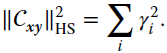
This quantity is zero only in the case where there is no first‐order dependence between x and y. Note that the Hilbert–Schmidt norm is limited to the detection of first‐order relations, and thus more complex (higher order effects) cannot be captured.
The previous notion of covariance operator in the field of kernel functions and measures was proposed in (Gretton et al., 2005c). Essentially, assume a (non‐linear) mapping ![]() in such a way that the dot product between features is given by a positive definite kernel function Kx(x, x′) = 〈ϕ(x), ϕ(x′)〉. The feature space
in such a way that the dot product between features is given by a positive definite kernel function Kx(x, x′) = 〈ϕ(x), ϕ(x′)〉. The feature space ![]() has the structure of an RKHS. Assume another mapping
has the structure of an RKHS. Assume another mapping ![]() with associated kernel Ky(y, y′) = 〈ψ(y), ψ(y′)〉. Under these conditions, a conditions, a cross‐covariance operator between these mappings can be defined, similar to the covariance matrix in Equation 12.4. The cross‐covariance is a linear operator
with associated kernel Ky(y, y′) = 〈ψ(y), ψ(y′)〉. Under these conditions, a conditions, a cross‐covariance operator between these mappings can be defined, similar to the covariance matrix in Equation 12.4. The cross‐covariance is a linear operator ![]() of the form
of the form
where ⊗ is the tensor product, ![]() , and
, and ![]() . See more details in Baker (1973) and Fukumizu et al. (2004). The HSIC is defined as the squared norm of the cross‐covariance operator,
. See more details in Baker (1973) and Fukumizu et al. (2004). The HSIC is defined as the squared norm of the cross‐covariance operator, ![]() , and it can be expressed in terms of kernels (Gretton et al., 2005c):
, and it can be expressed in terms of kernels (Gretton et al., 2005c):

where ![]() is the expectation over both
is the expectation over both ![]() and an additional pair of variables
and an additional pair of variables ![]() drawn independently according to the same law.
drawn independently according to the same law.
Now, given a sample dataset Z = {(x1, y1), …, (xN, yN)} of size N drawn from ![]() xy, an empirical estimator of HSIC is (Gretton et al., 2005c)
xy, an empirical estimator of HSIC is (Gretton et al., 2005c)
where Tr is the trace (the sum of the diagonal entries), Kx and Ky are the kernel matrices for the data x and the labels y respectively, and Hij = δij − (1/N) centers the data and the label features in ![]() and
and ![]() . Here, δ represents the Kronecker symbol, where δij = 1 if i = j, and zero otherwise.
. Here, δ represents the Kronecker symbol, where δij = 1 if i = j, and zero otherwise.
Summarizing, HSIC (Gretton et al., 2005c) is a simple yet very effective method to estimate statistical dependence between random variables. HSIC corresponds to estimating the norm of the cross‐covariance in ![]() , whose empirical (biased) estimator is HSIC := [1/(N − 1)2]Tr(KxKy), where Kx and Ky are kernels working on data from sets
, whose empirical (biased) estimator is HSIC := [1/(N − 1)2]Tr(KxKy), where Kx and Ky are kernels working on data from sets ![]() and
and ![]() . It can be shown that, if the RKHS kernel is universal, such as the RBF or Laplacian kernels, HSIC asymptotically tends to zero when the input and output data are independent, and HSIC = 0 if
. It can be shown that, if the RKHS kernel is universal, such as the RBF or Laplacian kernels, HSIC asymptotically tends to zero when the input and output data are independent, and HSIC = 0 if ![]() . Note that, in practice, the actual HSIC is the Hilbert–Schmidt norm of an operator mapping between potentially infinite‐dimensional spaces, and thus would give rise to an infinitely large matrix. However, due to the kernelization, the empirical HSIC only depends on computable matrices of size N × N. We will come back to the issue of computational cost later.
. Note that, in practice, the actual HSIC is the Hilbert–Schmidt norm of an operator mapping between potentially infinite‐dimensional spaces, and thus would give rise to an infinitely large matrix. However, due to the kernelization, the empirical HSIC only depends on computable matrices of size N × N. We will come back to the issue of computational cost later.
Relation between Hilbert–Schmidt Independence Criterion and Maximum Mean Discrepancy
In Chapter 11 we introduced the MMD for hypothesis testing. We can show that MMD is related to HSIC. Let us define the product space ![]() with a kernel 〈ϕ(x, y), ϕ(x′, y′)〉 = K((x, y), (x′, y′)) = K(x, y)L(x′, y′), and the mean elements are given by
with a kernel 〈ϕ(x, y), ϕ(x′, y′)〉 = K((x, y), (x′, y′)) = K(x, y)L(x′, y′), and the mean elements are given by
and
Therefore, the MMD between these two mean elements is
Relation between Hilbert–Schmidt Independence Criterion and Other Kernel Dependence Measures
HSIC was not the first kernel dependence estimate presented in the literature. Actually, Bach and Jordan (2002) derived a regularized correlation operator from the covariance and cross‐covariance operators, and its largest singular value (the KCCA) was used as a statistic to test independence. Later, Gretton et al. (2005a) proposed the largest singular value of the cross‐covariance operator as an efficient alternative that needs no regularization. This test is called the constrained covariance (COCO) (Gretton et al., 2005a). A variety of empirical kernel quantities derived from bounds on the mutual information that hold near independence were also proposed, namely the kernel generalized variance (KGV) and the kernel mutual information (kMI) (Gretton et al., 2005b). Later, HSIC (Gretton et al., 2005c) was introduced, hence extending COCO by using the entire spectrum of the cross‐covariance operator, not just the largest singular value. As we have seen, a related statistic is the MMD criterion, which tests for statistical differences between embeddings of probability distributions into RKHS. When MMD is applied to the problem of testing for independence, the test statistic reduces to HSIC. A simple comparison between all the methods treated in this section is given in Figure 12.4. Listing 12.2 gives a simple MATLAB implementation comparing Pearson’s correlation and HSIC in this particular example. The book’s repository provides MATLAB tools and links to relevant toolboxes on (kernel) dependence estimation.
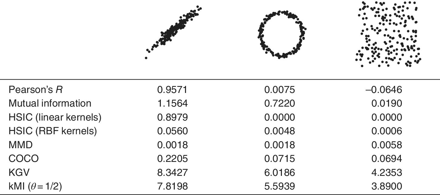
Figure 12.4 Dependence estimates for three examples revealing (left) high correlation (and hence high dependence), (middle) high dependence but null correlation, and (right) zero correlation and dependence. The Pearson correlation coefficient R and linear HSIC only capture second‐order statistics (linear correlation), while the rest capture in general higher order dependences. Note that, for MMD, the higher the more divergent (independent), while KGV upper bounds kMI and mutual information.
Relations between Hilbert–Schmidt Independence Criterion and the Kernel Multivariate Analysis Framework
HSIC constitutes an interesting framework to study KMVA methods for dimensionality reduction. We summarize the relations between the methods under the HSIC perspective in Table 12.2. For instance, HSIC reduces to PCA for the case of linear kernels. Recall that PCA reduces to find an orthogonal projection matrix V such that the projected data, XV, preserves the maximum variance; that is, ![]() subject to VTV = I, which may be written as follows:
subject to VTV = I, which may be written as follows:
Therefore, PCA can be interpreted as finding V such that its linear kernel has maximum dependence with the kernel obtained from the original data. Assuming that X is again centered, there is no need for including the centering matrix H in the HSIC estimate.
Table 12.2 Relation between dimensionality reduction methods and HSIC, HSIC := Tr(HKxHKy), where all techniques use the orthogonality constraint YTY = I.
| Method | Kx | Ky | Comments |
| PCA (Jolliffe, 1986) | XXT | YYT | — |
| KPCA (Schölkopf et al., 1998) | Kx | YYT | Typically RBF kernels used |
| Maximum variance unfolding (MVU) (Song et al., 2007) | Kx | LLT | Subject to positive definiteness Kx ≽ 0, preservation of local distance structure |
| Multidimensional scaling (MDS) (Cox and Cox, 1994) | YYT | D is the matrix of all pairwise Euclidean distances | |
| Isomap (Tenenbaum et al., 2000) | YYT | Dg is the matrix of all pairwise geodesic distances | |
| Locally linear embedding (LLE) (Roweis and Saul, 2000) | L†, or λmaxI − L | YYT | L = (I − V)(I − V)T, where V is the matrix of locally embedded weights |
| Laplacian eigenmaps (Belkin and Niyogi, 2003) | L†, or λmaxI − L | YYT | L = D − W, where W is a positive symmetric affinity matrix and D is the corresponding degree matrix |
From HSIC, one can also reach KPCA (Schölkopf et al., 1998) by using a kernel matrix K for the data X and requiring the second random variable y to be orthogonal and unit norm; that is:
where Y is any real‐valued matrix of size N × d. Note that KPCA does not require any other constraint imposed on Y, but for other KMVA methods, as well as for clustering and metric learning techniques, one may require to design Y to include appropriate restrictions.
Maximizing HSIC has also been used in dimensionality reduction with (colored) MVU (Song et al., 2007). This manifold learning method maximizes HSIC between source and target data, and accounts for the manifold structure by imposing local distance constraints on the kernel. In the original version of the MVU, a kernel K is learned via maximizing Tr(K) subject to some constraints. Assuming a similarity/dissimilarity matrix B, one can modify the original MVU by maximizing Tr(KB) instead of Tr(K) subject to the same constraints. This way, one simultaneously maximizes the dependence between the learned kernel K and the kernel B storing our side information. Note that, in this formulation, we center matrix K via one of the constraints in the problem, and thus can exclude matrix H in the empirical estimation of HSIC.
The HSIC framework can also help us to analyze relations to standard dimensionality reduction methods like MDS (Cox and Cox, 1994), Isomap (Tenenbaum et al., 2000), LLE (Roweis and Saul, 2000) and Laplacian eigenmaps (Belkin and Niyogi, 2003) depending on the definition of the kernel K used in Equation 12.7. Ham et al. (2004) pointed out the relation between KPCA and these methods.
Hilbert–Schmidt Component Analysis
The HSIC empirical estimate can be specifically incorporated in feature extraction schemes. For example, the so‐called HSCA method in Daniušis and Vaitkus (2009) iteratively seeks for projections that maximize dependence with the target variables and simultaneously minimize the dependence with previously extracted features, both in HSIC terms. This can be seen as a Rayleigh coefficient that leads to the iterative resolution of the following generalized eigendecomposition problem:
where Kf is a kernel matrix of already extracted projections in the previous iteration. Note that if one is only interested in maximizing source–target dependence in HSIC terms, and uses a linear kernel for the targets Ky = YYT, the problem reduces to
which interestingly is the same problem solved by KOPLS (see Table 12.1). The equivalence means that features extracted with KOPLS are those that maximize statistical dependence (measured by HSIC) between the projected source data and the target data (Izquierdo‐Verdiguier et al., 2012).
Kernel Dimensionality Reduction
KDR is a supervised feature extraction method that seeks a linear transformation of the data such that it maximizes the conditional HSIC on the labels. Notationally, the input data matrix ![]() , the output (label) matrix is
, the output (label) matrix is ![]() , and
, and ![]() is a projection matrix from the d‐dimensional space to a r‐dimensional space, r ≤ d. Hence, the linear projection is Z = XW, which is constrained to be orthogonal; that is, WTW = I. The optimal W in HSIC terms is obtained by solving the constrained problem
is a projection matrix from the d‐dimensional space to a r‐dimensional space, r ≤ d. Hence, the linear projection is Z = XW, which is constrained to be orthogonal; that is, WTW = I. The optimal W in HSIC terms is obtained by solving the constrained problem
This approach has been followed for both supervised and unsupervised settings:
- Fukumizu et al. (2003, 2004) introduced KDR under the theory of covariance operators (Baker, 1973). KDR reduces to the KGV introduced by Gretton et al. (2005b) as a contrast function for ICA, in which the goal is to minimize mutual information. They showed that KGV is in fact an approximation of the mutual information among the recovered sources around the factorized distributions. The interest in KDR is different: the goal is to maximize the mutual information as a good proxy to the problem of dimensionality reduction. Interestingly, the computational problem involved in KDR is the same as in KICA (Bach and Jordan, 2002).
- The unsupervised KDR (Wang et al., 2010) reduces to seeking W such that the signal X and its (regression‐based) approximation
 are mutually independent, given the projection; that is
  . The unsupervised KDR method then reduces to
 .
.The problem is typically solved by gradient‐descent techniques with line search, which constrains the projection matrix W to lie on the Grassmann–Stiefel manifold of WTW = I.
Let us illustrate the performance of the supervised KDR compared with other linear dimensionality reduction methods for the Wine dataset, which is a 13‐dimensional problem obtained from the UCI repository (http://archive.ics.uci.edu/ml/), where here it is used to illustrate projection onto a 2D subspace. Figure 12.5 shows the projection onto the 2D subspace estimated by each method. This example illustrates that optimizing HSIC to achieve linear separability is an alternative valid approach to maximize input–output covariance (PLS) or maximize correlation (CCA). Figure 12.5 can be reproduced by downloading the corresponding MATLAB toolboxes from the book’s repository and executing the script Demo_Fig_14_4.m in the supplementary material provided. A simplified version of the code is shown in Listing 12.3.

Figure 12.5 Projections obtained by different linear projection methods on the Wine data available at the UCI repository (http://archive.ics.uci.edu/ml/). Black and two different grey intensities represent three different classes.
12.3.2 Blind Source Separation Using Kernels
Extracting sources from observed mixed signals without supervision is the problem of BSS; see Chapter 2 for an introductory review to the field. Several approaches exist in the literature to solve the problem, but most of them have relied on ICA (Comon 1994; Gutmann et al. 2014; Hyvärinen et al. 2001). ICA seeks for a basis system where the dimensions of the signal are as independent as possible. Kernel dependence estimates based either on KCCA or HSIC have given rise to kernelized versions of ICA, leveraging better performance at the cost of higher computational cost. An alternative approach to ICA‐like techniques consists of exploiting second‐order BSS methods in an RKH,S like finding orthonormal basis of the submanifold formed by kernel‐mapped data (Harmeling et al., 2003).
Independent Component Analysis
The instantaneous noise‐free ICA model takes the form X = sA, where ![]() is a matrix containing N observations of s sources,
is a matrix containing N observations of s sources, ![]() is the mixing matrix (assumed to have full rank), and
is the mixing matrix (assumed to have full rank), and ![]() contains the observed mixtures. We denote as s and x single rows of matrices S and X respectively, and si is the ith source in s. ICA is based on the assumption that the components si of components si of s, for all i = 1, …, s are mutually statistically independent; that is, the observed vector x depends only on the source vector s at each instant and the source samples s are drawn independently and identically from the pdf
contains the observed mixtures. We denote as s and x single rows of matrices S and X respectively, and si is the ith source in s. ICA is based on the assumption that the components si of components si of s, for all i = 1, …, s are mutually statistically independent; that is, the observed vector x depends only on the source vector s at each instant and the source samples s are drawn independently and identically from the pdf ![]() s. As a conclusion, the mixture samples x are likewise drawn independently and identically from the pdf
s. As a conclusion, the mixture samples x are likewise drawn independently and identically from the pdf ![]() x. The task of ICA is to recover the independent sources via an estimate
x. The task of ICA is to recover the independent sources via an estimate ![]() of the inverse of the mixing matrix A such that the recovered signals
of the inverse of the mixing matrix A such that the recovered signals ![]() have mutually independent components. When the sources s are Gaussian, A can be identified up to an ordering and scaling of the recovered sources via a permutation matrix
have mutually independent components. When the sources s are Gaussian, A can be identified up to an ordering and scaling of the recovered sources via a permutation matrix ![]() and a scaling matrix D. Very often the mixtures X are pre‐whitened via PCA,
and a scaling matrix D. Very often the mixtures X are pre‐whitened via PCA, ![]() , so
, so ![]() , where W contains the whitened observations. Now, assuming that the sources si have zero mean and unit variance, AV is orthogonal and the unmixing model becomes Y = WQ, where Q is an orthogonal unmixing matrix (QQT = I) and
, where W contains the whitened observations. Now, assuming that the sources si have zero mean and unit variance, AV is orthogonal and the unmixing model becomes Y = WQ, where Q is an orthogonal unmixing matrix (QQT = I) and ![]() contains the estimates of the sources. The idea of ICA can also be employed for optimizing CCA‐like problems (for instance, see Gutmann et al. (2014)), where higher order relations are taken into account in order to find the basis to represent different datasets in a canonical space.
contains the estimates of the sources. The idea of ICA can also be employed for optimizing CCA‐like problems (for instance, see Gutmann et al. (2014)), where higher order relations are taken into account in order to find the basis to represent different datasets in a canonical space.
Kernel Independent Component Analysis Using Kernel Canonical Correlation Analysis
The original version of KICA was introduced by Bach and Jordan (2005b), and uses a KCCA‐based contrast function to obtain the unmixing matrix W. For “rich enough” kernels, such as the Gaussian kernel, it was shown that the components of the random vector x are independent if and only if their first canonical correlation in the corresponding RKHS is equal to zero. KICA utilizes a gradient‐descent approach to minimize a KCCA‐based contrast function, taking into account that whitening the features will have the effect of that the unmixing matrix W will have orthonormal vectors. KICA has better performance than the previous three algorithms and also it is more robust against outliers and near‐Gaussianity of the sources. However, these performance improvements come at a higher computational cost. Figure 12.6 shows an example of using KICA to unmix signals that have been mixed using a linear combination. The example can be reproduced using the KICA toolbox linked in the book’s repository and the code in Listing 12.4.

Figure 12.6 Demixing example using KICA. From left to right we show the original source signals, the original (linearly) mixed signals, and the results obtained by KICA and ICA. We indicate the kurtosis in every dimension.
Kernel Independent Component Analysis Using Hilbert–Schmidt Independence Criterion
KICA based on minimizing HSIC as a contrast function has been recently introduced (Shen et al. 2007, 2009). The motivation is clear: in the ICA model, the components si of the sources s are mutually statistically independent if and only if their pdf factorizes ![]() . The problem in this assumption is that pairwise independence does not imply mutual independence (while it holds vice versa). The solution here is that, in the ICA setting, unmixed components can be uniquely identified using only the pairwise independence between components of the recovered sources Y, since pairwise independence between components of Y in this case implies their mutual independence (and thus recovery of the sources S). Hence, by summing all unique pairwise HSIC measures, an HSIC‐based contrast function over the estimated signals Y is defined as
. The problem in this assumption is that pairwise independence does not imply mutual independence (while it holds vice versa). The solution here is that, in the ICA setting, unmixed components can be uniquely identified using only the pairwise independence between components of the recovered sources Y, since pairwise independence between components of Y in this case implies their mutual independence (and thus recovery of the sources S). Hence, by summing all unique pairwise HSIC measures, an HSIC‐based contrast function over the estimated signals Y is defined as

where ![]() is the difference between the kth and the lth samples of the whitened observations, and
is the difference between the kth and the lth samples of the whitened observations, and ![]() represents the empirical expectation over all k and l. The expression of H(Q) reduces to just summing over all possible HSIC estimates of Y. Intuitively, one can see that the goal in KICA is to find an unmixing matrix Q such that the dependence between the estimated unmixed sources QTW is minimal in terms of the HSIC between all pairs of signals. The algorithm was first introduced by Bach and Jordan (2002), and later extended to a fast implementation known as FastKICA that uses an approximate Newton method to perform this optimization (Shen et al. 2007, 2009). The
represents the empirical expectation over all k and l. The expression of H(Q) reduces to just summing over all possible HSIC estimates of Y. Intuitively, one can see that the goal in KICA is to find an unmixing matrix Q such that the dependence between the estimated unmixed sources QTW is minimal in terms of the HSIC between all pairs of signals. The algorithm was first introduced by Bach and Jordan (2002), and later extended to a fast implementation known as FastKICA that uses an approximate Newton method to perform this optimization (Shen et al. 2007, 2009). The fastKICA package is a convenient implementation of the method.
Kernel Blind Source Separation
The previous approaches are based on introducing kernel dependence estimates as contrast functions in ICA. Alternatively, one can follow the standard “kernelization” procedure: first the data are (implicitly) mapped to a high (possibly infinite)‐dimensional kernel feature space, and then a linear algorithm is defined and solved (implicitly) therein by means of the kernel trick. Let us review the two main approaches available in the literature, and their relations to KMVA.
Harmeling et al. (2003) followed the standard kernelization of BSS based on second‐order statistics. In particular, the method exploits temporal decorrelation in Hilbert spaces via the time‐delayed second‐order projection (TDSEP) technique, which relies on simultaneous diagonalization techniques to perform linear blind source separation on the projected data. Therefore, one obtains a number of linear directions of separated nonlinear components in input space. The algorithm was coined kernel TDSEP. After embedding, data form a smaller submanifold in feature space, which is typically smaller than the number of training data points. The approach then tries to adapt to this sort of effective dimension as a preprocessing step and to construct an orthonormal basis of this submanifold. This first step performs standard dimensionality reduction.
In particular, Harmeling et al. (2003) proposed to construct an orthonormal basis in feature spaces from a subset of selected data points therein. Given T observed signals  , and N vectors
  , we define the corresponding kernel matrices Kx = ΦxΦxT and Kx = ΦvΦvT. Now let us assume that the span of Φx is the same as the span of Φv and the rank of Φv is N. Since Φv constitutes a basis, Kv is full rank and has an inverse. The orthonormal basis can thus be defined as V = (ΦvΦvT)−1/2Φv, and hence projecting new data onto the basis reduces simply to Ψx[t] = (ΦvΦvT)−1/2ΦvΦxT[t] = Kv−1Kvx. The definition of the basis could be actually done extracting actually done extracting the most relevant directions in kernel feature spaces via the diagonalization of the full kernel matrix; that is, via KPCA. Nevertheless, the alternative approach to form the basis is very useful for making the subsequent application of BSS linear methods computationally and
Kernel Entropy Component Analysis
Kernel entropy component analysis (KECA) was proposed by Jenssen (2010, 2013) to implement a feature extractor according to the entropy components. KECA, like KPCA, is a spectral method based on the kernel similarity matrix. Nevertheless, KECA does not necessarily use the top eigenvalues and eigenvectors of the kernel matrix. Unlike KPCA, which preserves maximally the second‐order statistics of the dataset, KECA is founded on information theory and tries to preserve the maximum Rényi entropy of the input space dataset. KECA has proven useful in, for example, remote sensing (Gómez‐Chova et al., 2012; Luo and Wu, 2012; Luo et al., 2014), face recognition (Shekar et al., 2011), and some other applications (Hu et al. 2013; Jiang et al. 2013; Xie and Guan 2012). Several extensions have been proposed for feature selection (Zhang and Hancock, 2012), class‐dependent feature extraction (Cheng et al., 2014), and SSL as well (Myhre and Jenssen, 2012).
The KECA algorithm relies on the eigendecomposition of the (uncentered) kernel matrix, and sorts the eigenvectors according to the entropy values of the projections. Given a dataset ![]() of dimensionality d, the entropy may be estimated through kernel density estimation (Silverman, 1986) as
of dimensionality d, the entropy may be estimated through kernel density estimation (Silverman, 1986) as ![]() , where V2 is the so‐called information potential (Principe, 2010):
, where V2 is the so‐called information potential (Principe, 2010):
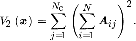
In this expression, Nc ≤ N is the number or retained components and the matrix A is obtained from the (N × N) kernel or Gram matrix K whose entries are the kernel function values K(xi, xj). Equation 12.12 is based on the kernel decomposition introduced in Jenssen (2010):

where E contains the eigenvectors in columns, E = [e1|⋯|eN], and D is a diagonal matrix containing the eigenvalues of K; that is, Dii = λi. An illustrative MATLAB code snippet for KECA is provided in Listing 12.5.
KECA uses the Rényi entropy to sort the basis extracted by PCA. A novel proposal (Izquierdo‐Verdiguier et al., 2016), the optimized KECA (OKECA) method, looks directly for the basis that maximizes the Rényi entropy, therefore maximizing the information using as few components as possible. OKECA is based on a similar idea to ICA, and optimizes an extra rotation matrix on top of PCA directions. The new kernel matrix decomposition is expressed as

where W is an orthonormal linear transformation; that is, QQT = I. In order to solve the OKECA decomposition, OKECA resorts to a gradient‐ascent approach. Note that OKECA is more computationally demanding than KECA because not only requires an eigendecomposition of a kernel matrix but also the gradient ascent procedure to refine the final features. An illustrative MATLAB code snippet for OKECA is provided in Listing 12.6.
In general, both KECA and OKECA are different from (but still intimately related to) KMVA methods. On the one hand, they maintain a probabilistic input space interpretation, seek to capture the entropy of the data in a reduced number of components, and constitute a convergence point between kernel methods and information theoretic learning (Jenssen, 2009). On the other hand, KPCA, KCCA, and KPLS maximize the variance, correlation, or alignment (covariance) with the output variables in kernel feature space respectively. The similarities between these methods arise from the use of a kernel function and from the exploitation of the spectral (eigenvalues and eigenvectors) properties of the corresponding kernel matrices. KECA and OKECA can be used for density estimation. As explained by Girolami (2002b), if the decomposition of the uncentered kernel matrix follows the form K = EDET, where E is orthonormal and D is a diagonal matrix, then the kernel‐based density estimation may be expressed as
where ![]() is the reduced version of E by keeping columns for nf < N, and as usual k* := [K(x*, x1), …, K(x*, xN)]T. Therefore, density estimation
is the reduced version of E by keeping columns for nf < N, and as usual k* := [K(x*, x1), …, K(x*, xN)]T. Therefore, density estimation ![]() can be readily done by fixing a number of extracted features nf. Figure 12.7 illustrates the ability of KECA and OKECA for density estimation in a ring distribution. Note that OKECA concentrates most of the entropy information in the first projection. This agrees with the fact that few components are needed to obtain a good pdf estimation. On the contrary, KECA cannot estimate correctly the pdf using only the first component and actually needs at least five components. We show results for two standard ways to estimate the σ length‐scale parameter: an ML strategy, σML following Duin (1976), and setting σ to 15% of the median distance between points following prescriptions in Jenssen (2010). In both cases OKECA outperforms KECA.
can be readily done by fixing a number of extracted features nf. Figure 12.7 illustrates the ability of KECA and OKECA for density estimation in a ring distribution. Note that OKECA concentrates most of the entropy information in the first projection. This agrees with the fact that few components are needed to obtain a good pdf estimation. On the contrary, KECA cannot estimate correctly the pdf using only the first component and actually needs at least five components. We show results for two standard ways to estimate the σ length‐scale parameter: an ML strategy, σML following Duin (1976), and setting σ to 15% of the median distance between points following prescriptions in Jenssen (2010). In both cases OKECA outperforms KECA.

Figure 12.7 Density estimation for the ring dataset by KECA and OKECA using different number of extracted features n and estimates of the kernel length‐scale parameter σ (ML or squared distance). Black color represents low pdf values and yellow color high pdf values.
12.4 Extensions for Large‐Scale and Semi‐supervised Problems
An important problem in kernel‐based feature extraction is related to the computational cost. Since Kx is of size N × N, method complexity scales quadratically with N in terms of memory, and cubically with respect to the computation time. The opposite situation often occurs as well: when N is small, the extracted features may be useless, especially for high‐dimensional ![]() (Abrahamsen and Hansen, 2011). These issues limit the applicability of kernel‐based feature extraction methods in real‐life scenarios with either very large or very small labeled datasets. We next summarize some extensions to deal with large‐scale problems and semi‐supervised situations in which few labeled data are available.
(Abrahamsen and Hansen, 2011). These issues limit the applicability of kernel‐based feature extraction methods in real‐life scenarios with either very large or very small labeled datasets. We next summarize some extensions to deal with large‐scale problems and semi‐supervised situations in which few labeled data are available.
12.4.1 Efficiency with the Incomplete Cholesky Decomposition
Very often, feature extraction methods on kernels rely on the calculation of traces on products of kernel matrices; for instance, see HSCA or KICA that try to maximize the HSIC measure between some random variables. This operation is simple yet computationally demanding when a high number of samples are available. In order to speed this operation up, one can rely on sparse approximations of the basis spanning the solution (as we will see in the next section), by intelligent dataset subsampling (e.g., via AL), or Nyström approximations of the kernel matrices. A convenient alternative is to exploit low‐rank approximations of the kernel matrices via Cholesky decomposition.
Notationally, given two kernel matrices K1 and K2, the cost associated with the operation Tr(K1K2) can be greatly reduced via incomplete Cholesky estimation. An incomplete Cholesky decomposition of a Gram matrix Ki yields a low‐rank approximation, ![]() that greedily minimizes
that greedily minimizes ![]() . The cost of computing the N × r matrix Gi is
. The cost of computing the N × r matrix Gi is ![]() , with r ≪ N. Greater values of r result in a more accurate reconstruction of Ki. Interestingly, it is well known that the spectrum of a Gram matrix based on the (RBF) Gaussian kernel generally decays rapidly, and a small r yields a very good approximation. Plugging the Cholesky eigendecomposition of the two kernels leads to
, with r ≪ N. Greater values of r result in a more accurate reconstruction of Ki. Interestingly, it is well known that the spectrum of a Gram matrix based on the (RBF) Gaussian kernel generally decays rapidly, and a small r yields a very good approximation. Plugging the Cholesky eigendecomposition of the two kernels leads to
which involves an equivalent trace of a much smaller matrix, so we can avoid computing the N × N matrices and just do r1 × r2 matrix calculations. This technique has been widely used in KMVA and also in kernel dependence estimation methods such as the HSIC (Gretton et al., 2005b).
12.4.2 Efficiency with Random Fourier Features
We have already seen the effectiveness of approximating shift‐invariant kernels, using projections on random Fourier features (Rahimi and Recht, 2007, 2009). This technique was illustrated in classification and regression settings; see Section 10.4.2. Let us show the application of the approximation in HSIC presented in Pérez‐Suay and Camps‐Valls (2017). Following previous notation, recall that ![]() can be approximated with the explicitly mapped data via
can be approximated with the explicitly mapped data via ![]() , and collectively grouped in the matrix
, and collectively grouped in the matrix ![]() , and will be denoted as
, and will be denoted as ![]() . The familiar SE Gaussian kernel
. The familiar SE Gaussian kernel ![]() can be approximated using D random features,
can be approximated using D random features, ![]() , 1 ≤ i ≤ D. The randomized HSIC (RHSIC) for fast dependence estimation in large‐scale problems is developed as follows: kernel matrices Kx and Ky are approximated using complex exponentials of projected data matrices,
, 1 ≤ i ≤ D. The randomized HSIC (RHSIC) for fast dependence estimation in large‐scale problems is developed as follows: kernel matrices Kx and Ky are approximated using complex exponentials of projected data matrices, ![]() and
and ![]() and
and ![]() , where
, where ![]() , both drawn from a Gaussian. Now, plugging the corresponding kernel approximations,
, both drawn from a Gaussian. Now, plugging the corresponding kernel approximations, ![]() and
and ![]() , into Equation 12.7, and after manipulating terms, we obtain
, into Equation 12.7, and after manipulating terms, we obtain
which corresponds to the Hilbert–Schmidt norm of the randomized cross‐covariance operator, ![]() , which can be computed explicitly and just once. The computational complexity of RHSIC reduces considerably over the original HSIC. A naive implementation of HSIC runs
, which can be computed explicitly and just once. The computational complexity of RHSIC reduces considerably over the original HSIC. A naive implementation of HSIC runs ![]() , while the RHSIC cost is
, while the RHSIC cost is ![]() , where D = Dx = Dy, since computing matrices Z only involves matrix multiplications and exponentials. We want to note that other KMVA methods have enjoyed use of this randomization technique to expedite performance, such as KCCA and KPCA (López‐Paz et al., 2014).
, where D = Dx = Dy, since computing matrices Z only involves matrix multiplications and exponentials. We want to note that other KMVA methods have enjoyed use of this randomization technique to expedite performance, such as KCCA and KPCA (López‐Paz et al., 2014).
12.4.3 Sparse Kernel Feature Extraction
To address the problems of large‐scale computation and dense solutions in KMVA, several solutions have been proposed. The family of KMVA sparse methods tries to obtain solutions that can be expressed as a combination of a reduced subset of the training data, and therefore require only r kernel evaluations per sample (being r ≪ N) for feature extraction. In contrast to the many linear MVA algorithms that induce sparsity with respect to the original variables, we will only review methods attaining sparse solutions in terms of the samples (i.e., sparsity in the αi vectors).
Roughly speaking, sparsification methods can be classified into low‐rank approximation methods that aim at working with reduced r × r matrices (r ≪ N), and reduced set methods that work with N × r matrices. Following the first approach, the Nyström low‐rank approximation of an N × N kernel matrix KNN is expressed as ![]() , where subscripts indicate row and column dimensions. This method was first used in Gaussian processes, and later by Hoegaerts et al. (2005) in order to approximate the feature mapping instead of the kernel, which leads to sparse versions of KPLS and KCCA.
, where subscripts indicate row and column dimensions. This method was first used in Gaussian processes, and later by Hoegaerts et al. (2005) in order to approximate the feature mapping instead of the kernel, which leads to sparse versions of KPLS and KCCA.
Among the reduced set methods, a sparse KPCA (sKPCA) was proposed by Tipping (2001), where the sparsity in the representation is obtained by assuming a generative model for the data in ![]() that follows a normal distribution and includes a noise term with variance vn. The ML estimation of the covariance matrix is shown to depend on just a subset of the training data, and so it does the resulting solution. A sparse KPLS (sKPLS) was introduced by Momma and Bennett (2003). The method computes the projections with a reduced set of the training samples. Each one of the projections is found using a loss that is similar to the ε insensitive loss used in SVR. The sparsification is induced via a multistep adaptation with high computational burden.
that follows a normal distribution and includes a noise term with variance vn. The ML estimation of the covariance matrix is shown to depend on just a subset of the training data, and so it does the resulting solution. A sparse KPLS (sKPLS) was introduced by Momma and Bennett (2003). The method computes the projections with a reduced set of the training samples. Each one of the projections is found using a loss that is similar to the ε insensitive loss used in SVR. The sparsification is induced via a multistep adaptation with high computational burden.
The algorithms in Tipping (2001) and Momma and Bennett (2003), however, still require the computation of the full kernel matrix during the training.
A reduced complexity KOPLS (rKOPLS) was proposed by Arenas‐García et al. (2007) by imposing sparsity in the projection vectors representation a priori, ![]() , where Φr is a subset of the training data containing r samples (r ≪ N) and β is the new argument for the maximization problem, which now becomes
, where Φr is a subset of the training data containing r samples (r ≪ N) and β is the new argument for the maximization problem, which now becomes

Since kernel matrix KrN = ΦrΦT involves the inner products in ![]() of all training points with the patterns in the reduced set, this method still takes into account all data during the training phase, and is therefore different from simple subsampling. This “sparsification” procedure avoids the computation of the full kernel matrix at any step of the algorithm. An additional advantage of this method is that matrices
of all training points with the patterns in the reduced set, this method still takes into account all data during the training phase, and is therefore different from simple subsampling. This “sparsification” procedure avoids the computation of the full kernel matrix at any step of the algorithm. An additional advantage of this method is that matrices ![]() and
and ![]() are both of size r × r, and they can be computed as sums over the training data. This fact makes the storage space grow quadratically with r. Also, there is an implicit regularization imposed by the sparsification, which decreases the overfitting risk of the method. Reduced complexity versions of KPCA and KKCA are shown in the experimental section that use the same sparsification method, and will be referred as rKPCA and rKCCA.
are both of size r × r, and they can be computed as sums over the training data. This fact makes the storage space grow quadratically with r. Also, there is an implicit regularization imposed by the sparsification, which decreases the overfitting risk of the method. Reduced complexity versions of KPCA and KKCA are shown in the experimental section that use the same sparsification method, and will be referred as rKPCA and rKCCA.
Interestingly, the extension to KPLS2 is not straightforward, since the deflation step would still require the full kernel matrix KNN. Alternatively, two sparse KPLS schemes were presented by Dhanjal et al. (2009) under the name of sparse maximal alignment (SMA) and sparse maximal covariance (SMC). Here, KPLS iteratively estimates projections that either maximize the kernel alignment or the covariance of the projected data and the true labels.
Table 12.3 summarizes some computational and implementation issues of the aforementioned sparse KMVA methods, and of standard nonsparse KMVA and linear methods. Some aspects that can be helpful to choose an algorithm for a particular application can be obtained from an analysis of the properties of each algorithm. An important step is to choose an adequate kernel and parameters. KMVA methods can be adjusted using cross‐validation to reduce overfitting at the expense of an increased computational burden, but regularization through sparsification can help to further reduce overfitting. Also, most methods can be implemented as either eigenvalue or generalized eigenvalue problems, whose complexity typically scales cubically with the size of the matrices analyzed. Therefore, both for memory and computational reasons, only linear MVA and the sparse approaches from Arenas‐García et al. (2007) and Dhanjal et al. (2009) are affordable when dealing with large datasets. A final advantage of sparse KMVA is the reduced number of kernel evaluations to extract features for new out‐of‐the‐sample data.
Table 12.3 Main properties of (K)MVA methods. Computational complexity and implementation issues are categorized for the considered dense and sparse methods in terms of the free parameters, number of kernel evaluations (KEs) during training, and storage requirements. Notation: N refers to the size of the labeled dataset, while d and m are the dimensions of the input and output spaces respectively.
| Method | Parameters | KE (training) | Storage requirements |
| PCA | None | None | |
| PLS | None | None | |
| CCA | None | None | |
| OPLS | None | None | |
| KPCA | Kernel | N2 | |
| KPLS | Kernel | N2 | |
| KCCA | Kernel | N2 | |
| KOPLS | Kernel | N2 | |
| sKPCA (Tipping, 2001) | Kernel, vn | N2 | |
| sKPLS (Momma and Bennett, 2003) | Kernel, ν, ε | N2 | |
| rKPCA | Kernel, r | rN | |
| rKCCA | Kernel, r | rN | |
| rKOPLS (Arenas‐García et al., 2007) | kernel, r | rN | |
| SMA/SMC (Dhanjal et al., 2009) | kernel, r | N2 |
12.4.4 Semi‐supervised Kernel Feature Extraction
When few labeled samples are available, the extracted features do not capture the structure of the data manifold well, which may lead to very poor results. SSL approaches have been introduced to alleviate these problems. Two approaches are encountered: the information conveyed by the unlabeled samples is either modeled with graphs or via kernel functions derived from generative clustering models.
Notationally, we are given l labeled and u unlabeled samples, a total of N = l + u. The semi‐supervised KCCA (ss‐KCCA) was introduced in Blaschko et al. (2011) by using the graph Laplacian. The method essentially solves the standard KCCA equations using kernel matrices computed with both labeled and unlabeled data, which are further regularized with the graph Laplacian:

where ![]() and
and ![]() . For the sake of notation compactness, subindices indicate the size of the corresponding matrices while superscripts denote whether they involve input or output data. Parameters αx, αy, γx, and γy trade off the contribution of labeled and unlabeled samples, and L = D−1/2(D − M)D1/2 represents the (normalized) graph Laplacian for the input and target domains, where D is the degree matrix whose entries are the sums of the rows of the corresponding similarity matrix M; that is,
. For the sake of notation compactness, subindices indicate the size of the corresponding matrices while superscripts denote whether they involve input or output data. Parameters αx, αy, γx, and γy trade off the contribution of labeled and unlabeled samples, and L = D−1/2(D − M)D1/2 represents the (normalized) graph Laplacian for the input and target domains, where D is the degree matrix whose entries are the sums of the rows of the corresponding similarity matrix M; that is, 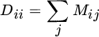 . It should be noted that for N = l and null regularization one obtains the standard KCCA (see Equation 12.3). Note also that this form of regularization through the graph Laplacian can be applied to any KMVA method. A drawback of this approach is that it involves tuning several parameters and working with larger matrices of size 2 N × 2 N, which can make its application difficult in practice.
Alternatively, cluster kernels – a form of generative kernel functions learned from data – have been used to develop semi‐supervised versions of kernel methods in general, and of KMVA methods in particular. The approach was used for KPLS and KOPLS by Izquierdo‐Verdiguier et al. (2012). Essentially, the method relies on combining a kernel function based on labeled information only, Ks(xi, xj), and a generative kernel directly learned by clustering all (labeled and unlabeled) data, Kc(xi, xj). Building Kc requires first running a clustering algorithm, such as EM assuming a GMM with different initializations, q = 1, …, Q, and with different number of clusters, g = 2, …, G + 1. This results in Q ⋅ G cluster assignments where each sample xi has its corresponding posterior probability vector ![]() . The probabilistic cluster kernel Kc is computed by averaging all the dot products between posterior probability vectors:
. The probabilistic cluster kernel Kc is computed by averaging all the dot products between posterior probability vectors:
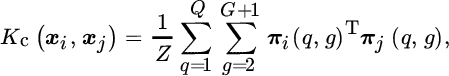
where Z is a normalization factor. The final kernel function is defined as the weighted sum of both kernels, K(xi, xj) = βKs(xi, xj) + (1 − β)Kc(xi, xj), where β ∈ [0, 1] is a scalar parameter to be adjusted. Intuitively, the cluster kernel accounts for probabilistic similarities at small and large scales (number of clusters) between all samples along the data manifold, and hence its name: the probabilistic cluster kernel (PCK) (Izquierdo‐Verdiguier et al., 2012). The method does not require computationally demanding procedures (e.g., current GMM clustering algorithms scale linearly with N), and the KMVA still relies just on the labeled data, and thus requires an l × N kernel matrix. All these properties are quite appealing from the practitioner’s point of view. Listing 12.7 gives a MATLAB code snippet showing how to compute the PCK. Note that this particular this particular kernel function is semi‐supervised and can be plugged into any kernel method.
Figure 12.8 shows an illustrative toy example evaluating the RBF, PCK, Fisher’s (Jaakkola et al., 1999), and Jensen–Shannon’s (Bicego et al., 2013) kernels. The data were generated by the composition of two normal distributions, ![]() and
and ![]() . We look at the structure of the kernel matrix through the first eigenvectors, and compute the Frobenius norm of the residuals with the ideal kernel. The length‐scale of the RBF was fixed to the average distance of all examples, while we used Q = 10 and G = 25 for Kc. The Fisher kernel used feature vectors extracted from a GMM using the same number of clusters as for the PCK, and the Jensen–Shannon kernel was built from divergence Jensen–Shannon obtained from Shannon entropy. Since the Fisher and Jensen–Shannon kernels are not intrinsically multiscale, here we implement a multiscale version of the Fisher and Jensen–Shannon kernels for the sake of a fair comparison. The figure shows that the PCK and the Jensen–Shannon return more discriminative eigenvectors and substantially different from the Fourier‐like basis obtained by the RBF and the Fisher kernel. The PCK better captures the local structure than the Jensen–Shannon kernel does. This clearly draws from the visual comparison of the kernel matrices, which is also supported by the Frobenius norm of the differences to the ideal kernel (Figure 12.8, given in parentheses).
. We look at the structure of the kernel matrix through the first eigenvectors, and compute the Frobenius norm of the residuals with the ideal kernel. The length‐scale of the RBF was fixed to the average distance of all examples, while we used Q = 10 and G = 25 for Kc. The Fisher kernel used feature vectors extracted from a GMM using the same number of clusters as for the PCK, and the Jensen–Shannon kernel was built from divergence Jensen–Shannon obtained from Shannon entropy. Since the Fisher and Jensen–Shannon kernels are not intrinsically multiscale, here we implement a multiscale version of the Fisher and Jensen–Shannon kernels for the sake of a fair comparison. The figure shows that the PCK and the Jensen–Shannon return more discriminative eigenvectors and substantially different from the Fourier‐like basis obtained by the RBF and the Fisher kernel. The PCK better captures the local structure than the Jensen–Shannon kernel does. This clearly draws from the visual comparison of the kernel matrices, which is also supported by the Frobenius norm of the differences to the ideal kernel (Figure 12.8, given in parentheses).

Figure 12.8 Example of differences between the local properties of the RBF, Jensen–Shannon kernel, Fisher’s kernel, and the PCK. We indicate in parentheses the Frobenius norm of the residuals with the ideal kernel,  .
.
12.5 Domain Adaptation with Kernels
Domain adaptation constitutes a field of high interest nowadays in pattern analysis and machine learning. Classification or regression algorithms developed with data from one domain cannot be directly used in another related domain, and hence adaptation of either the data representation or the classifier becomes strictly imperative (Quiñonero‐Candela et al., 2009; Sugiyama and Kawanabe, 2012). There is actually strong evidence that a significant degradation in the performance of state‐of‐the‐art image classifiers is due to test domain shifts such as changing image sensors and noise conditions (Saenko et al., 2010), pose changes (Farhadi and Tabrizi, 2008), consumer versus commercial video (Duan et al., 2012), and, more generally, datasets biased due to changing acquisition procedures (Torralba and Efros, 2011). Unlike in Hoffman et al. (2013), we focus on adapting data representations to facilitate the use of standard classifiers. Roughly speaking, domain adaptation solves a learning problem in a target domain by utilizing the training data in a different but related source domain. Intuitively, discovering a good feature representation across domains is crucial. The problem has captured the attention of researchers in many fields, also in the kernel methods community.
The signal‐ and image‐processing communities have also greatly contributed to this community, yet under different names. Domain adaptation is sometimes referred to as simply adaptation, transportability, inter‐calibration, or feature invariance learning. A collection of images must be compensated for illumination changes when a classifier must be used across domains, or speech signals from different users must be equalized for annotation and recognition steps. In general, data collected for the same problem in different instants, from different angles, by different systems and procedures show similar features but also reveal changes in their data manifold that need to be compensated before the direct exploitation. The problem is very challenging in high‐dimensional and low‐sized datasets, which is very often the case in signal‐processing problems.
Recently, several approaches have been proposed to learn a common feature representation for domain adaptation. Daumé III and Marcu (2011) presented a simple heuristic nonlinear mapping function to map the data from both source and target domains to a high‐dimensional feature space, where standard machine‐learning methods are used to train classifiers. On the other hand, Blitzer et al. (2006) proposed the so‐called structural correspondence learning algorithm to induce correspondences among features from the different domains. This method depends on the heuristic selections of pivot features that appear frequently in both domains. Although it is experimentally shown that structural correspondence learning can reduce the difference between domains based on the distance measure (Ben‐David et al., 2007), the heuristic criterion of pivot feature selection may be sensitive to different applications. Pan et al. (2008) proposed a new dimensionality reduction method, the so‐called maximum mean discrepancy embedding (MMDE), for domain adaptation. The method aims at learning a shared latent space underlying the domains where distance between distributions can be reduced. However, MMDE suffers from two major limitations: (1) MMDE is transductive, and does not generalize to out‐of‐sample patterns; (2) MMDE learns the latent space by solving a semi‐definite program (SDP), which is a very expensive optimization problem. Alternatives to these problems have been recently introduced in the literature.
Besides changing the data representation space via kernel feature extraction, another possibility is to correct for biases in the data distributions operating on the samples directly. The problem of covariate shift is intimately related to the problem of adaptation (Sugiyama and Kawanabe, 2012). Correcting for biases in the (changing) distributions can be addressed by upweighting and downweighting the relevance of the samples in the incoming target distribution. This technique has been widely exploited in many studies (Bickel et al. 2009; Huang et al. 2007; Kanamori et al. 2009): Huang et al. (2007) proposed the kernel mean matching (KMM) to reweight instances in an RKHS, Bickel et al. (2009) proposed to integrate the distribution correcting process into a kernelized logistic regression, and Kanamori et al. (2009) introduced a method called unconstrained LS importance fitting (uLSIF) to estimate sample relevance.
In this section, we review three examples of successful kernel methods for domain adaptation, each following different (yet obviously interconnected) philosophies: (1) sample reweighting strategies (KMM), (2) transfer component analysis (TCA), and (3) kernel manifold alignment (KEMA) for domain adaptation. Some illustrative examples of performance in signal processing tasks are given for illustration purposes.
12.5.1 Kernel Mean Matching
KMM is a kernel‐based method for sample reweighting. Note that, in general, learning methods typically try to minimize the expected risk, ![]() , where
, where ![]() is the pdf where samples are drawn from, and ℓ(x, y, θ) is the empirical loss function that depends that depends on a parameter θ. Since one typically has access only to pairs of examples (x, y) drawn from a density ℙ(x, y), the problem is solved by computing the empirical average over all available data,
is the pdf where samples are drawn from, and ℓ(x, y, θ) is the empirical loss function that depends that depends on a parameter θ. Since one typically has access only to pairs of examples (x, y) drawn from a density ℙ(x, y), the problem is solved by computing the empirical average over all available data, ![]() , which is normally regularized to avoid overfitting to the training set. However, the problem turns out to be more complex when the training and test probability functions differ, even slightly; that is,
, which is normally regularized to avoid overfitting to the training set. However, the problem turns out to be more complex when the training and test probability functions differ, even slightly; that is, ![]() . Actually, what one would desire is to minimize the
. Actually, what one would desire is to minimize the ![]() test(x, y), but one has only access to data drawn from
test(x, y), but one has only access to data drawn from ![]() train(x, y). The field of statistics known as importance sampling is concerned precisely with this problem: estimating properties of a particular distribution while only having samples generated from a estimating properties of a particular distribution while only having samples generated from a different distribution rather than the distribution of interest. The methods in this field are frequently used to estimate posterior densities or expectations in probabilistic models that are hard to treat analytically, as in
train(x, y). The field of statistics known as importance sampling is concerned precisely with this problem: estimating properties of a particular distribution while only having samples generated from a estimating properties of a particular distribution while only having samples generated from a different distribution rather than the distribution of interest. The methods in this field are frequently used to estimate posterior densities or expectations in probabilistic models that are hard to treat analytically, as in

provided that the support of ![]() test is contained in the support of
test is contained in the support of ![]() train. Therefore, we can compute the test risk from a modified version of the train risk, and this modification essentially translates into estimating the relevance parameter β per training example. This approach, however, involves density estimation of
train. Therefore, we can compute the test risk from a modified version of the train risk, and this modification essentially translates into estimating the relevance parameter β per training example. This approach, however, involves density estimation of ![]() train(x, y) and
train(x, y) and ![]() test(x, y), which in general is not an easy problem (recall Vapnik’s dictatum in Chapter 2). In addition, a deficient estimation of such densities may give rise to inaccurate estimates for the weights β, and consequently it may happen that the algorithm with adaptation mechanism works substantially worse than one without it. An alternative to both problems is given by the empirical KMM optimization.
test(x, y), which in general is not an easy problem (recall Vapnik’s dictatum in Chapter 2). In addition, a deficient estimation of such densities may give rise to inaccurate estimates for the weights β, and consequently it may happen that the algorithm with adaptation mechanism works substantially worse than one without it. An alternative to both problems is given by the empirical KMM optimization.
The KMM essentially tries to find weights ![]() in order to minimize the discrepancy between means subject to constraints βi ∈ [0, B] and
in order to minimize the discrepancy between means subject to constraints βi ∈ [0, B] and ![]() , which limits the discrepancy between
, which limits the discrepancy between ![]() train and
train and ![]() test, as well as ensure that β(x)
test, as well as ensure that β(x)![]() train(x) approaches a probability distribution. The objective function is given by the discrepancy term between the two empirical means. Using kernels [K]ij = K(xi, xj), and
train(x) approaches a probability distribution. The objective function is given by the discrepancy term between the two empirical means. Using kernels [K]ij = K(xi, xj), and 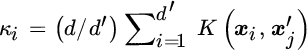 , one can check that
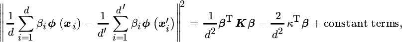
which reduces to solving a QP problem to optimize the weight vector β:

Note that KMM resembles the OC‐SVM using the ν‐trick, yet modified by the linear correction term involving κ, which measures sample relevance as well.
12.5.2 Transfer Component Analysis
TCA (Pan and Yang, 2011) tries to learn some transfer components across domains in an RKHS using the MMD measure (Borgwardt et al., 2006) introduced in Chapter 11 and related to the HSIC introduced before. In the subspace spanned by these transfer components, data distributions in different domains are close to each other. As a result, with the new representations in this subspace, one can apply standard machine‐learning methods to train classifiers or regression models in the source domain for use in the target domain. TCA does so in a very effective way. TCA essentially minimizes the distance between probability distributions of a source and a target domain. There are many distances in the literature to evaluate the difference between probability distributions: Kullback–Leibler divergence, Jensen–Shannon divergence, Bhattacharyya distance, and so on. However, these methods are affected by the data dimensionality, with the necessary probability density estimations becoming infeasible in high‐dimensional spaces.
TCA considers a setting where the target domain has plenty of unlabeled data. TCA also assumes that some labeled data are available in a source domain s, while only unlabeled data are available in the target domain t. Data will be denoted as belonging to either source or target domains with the corresponding superscript; that is, ![]() for the source and
for the source and ![]() for the target. The MMD estimate presented in Borgwardt et al. (2006) proposes a new indicator for comparing distributions based on the difference of the mean of the distributions computed in a common RKHS. This nonparametric measure is easily calculated no matter the number of variables describing the examples. Essentially, the empirical estimate of the MMD between the distribution of a given source dataset Xs and that of a related target dataset Xt is given by
for the target. The MMD estimate presented in Borgwardt et al. (2006) proposes a new indicator for comparing distributions based on the difference of the mean of the distributions computed in a common RKHS. This nonparametric measure is easily calculated no matter the number of variables describing the examples. Essentially, the empirical estimate of the MMD between the distribution of a given source dataset Xs and that of a related target dataset Xt is given by

The problem thus reduces to finding the nonlinear transformation ϕ(⋅) explicitly, which in principle is not possible. Instead, by using the kernel trick, one defines a reproducing kernel as K(xi, xj) = ϕ(xi)Tϕ(xj). It can be demonstrated that the problem of estimating the distance between the empirical means of the two domains reduces to
where

is a kernel matrix with Ns + Nt entries formed by three kernel matrices built on the data in the source domain Kss, target domain Ktt, and cross domains, Kst; and the matrix L is a positive semi‐definite matrix with entries ![]() if xi and xj belong to the source domain,
if xi and xj belong to the source domain, ![]() if xi and xj belong to the target domain, and Lij = 1/(NsNt) otherwise. Listing 12.8 gives an example for computing the MMD.
if xi and xj belong to the target domain, and Lij = 1/(NsNt) otherwise. Listing 12.8 gives an example for computing the MMD.
In the transductive setting, learning the kernel can be solved by learning the kernel matrix K instead. In Pan et al. (2008), the resultant kernel matrix learning problem is formulated as an SDP, and PCA is then applied on the learned kernel matrix to find a low‐dimensional latent space across domains. This is referred to as MMDE. Three main problems are devised with this approach. First, it is transductive and cannot generalize on unseen patterns. Second, the criterion to be optimized requires the kernel to be positive semi‐definite and the resultant kernel learning problem has to be solved by expensive SDP solvers.
TCA instead relies on kernel feature extraction to solve the problem and simply introduces the considerations (1) we want to optimize a projection matrix such that the MMD is minimized after transformation, and (2) the extractor should respect the main properties of the source and target data. For the first condition, and starting from the kernel matrix K given before, it is possible to use a projection matrix W to compute the kernel matrix between mapped samples as K = KWWTK. Afterwards, to obtain the MMD measure for the mapped samples, we simply have
which can be minimized with respect to W. For the second condition, the mapping ϕ should not harm the target supervised learning task by deforming too much the input space, so a regularization term is introduced able to preserve (and maximize) the initial data variance in the newly created subspace, ∥W∥2. Combining both terms, TCA reduces to solve
where Σ = WTKHKW is the covariance matrix of the projected data, H is a centering matrix in Hilbert spaces, H = I − 1/(NsNt)11T, and λ is a trade‐off parameter for tuning the influence of the regularization term and thus controlling the complexity of W. Such an optimization problem can be reformulated as a trace maximization problem yielding the following solution: the mapping matrix W is obtained by performing the eigendecomposition of
and keeping the r eigenvectors associated with the r largest eigenvalues. Once W is available, one can readily compute the r coordinates (the r uncorrelated transfer components) of the mapped samples as ![]() . In this latent subspace where distribution differences are reduced it is now possible to train a supervised classifier on the mapped source labeled samples and subsequently use it to classify the target image embedded in the same subspace. The reader may find MATLAB code for TCA in the book’s repository.
. In this latent subspace where distribution differences are reduced it is now possible to train a supervised classifier on the mapped source labeled samples and subsequently use it to classify the target image embedded in the same subspace. The reader may find MATLAB code for TCA in the book’s repository.
12.5.3 Kernel Manifold Alignment
The problem of aligning data manifolds reduces to finding projections between different sets of data, assuming that all lie on a common manifold. Roughly speaking, manifold alignment is a new form of MVA that dates back to the work of Hotelling in 1936 on CCA (Hotelling, 1936), where projections try to correlate the data sources onto a common target domain. The renewed concept of manifold alignment was first introduced by Ham et al. (2003), where a manifold constraint was added to the general problem of correlating sets of high‐dimensional vectors. The main problem of CCA, its kernel counterpart KCCA (Lai and Fyfe, 2000b), and many other domain adaptation methods (Blitzer et al. 2006; Daumé III and Marcu 2011; Duan et al. 2009, 2012; Ham et al. 2003) when confronted with manifold alignment problems is that, unfortunately, points in different sources must be corresponding pairs, which is often hard to meet in real applications. Actually, methods typically assume that the source and target domains are represented by the same features and instances, and try to match the only changing entity, namely the data distributions. Methods in the related field of transfer learning also commonly assume the availability of enough labeled data shared across domains (Dai et al., 2008; Pan and Yang, 2010); but again, this is a strong assumption in most of real‐life problems.
The problem of manifold alignment without correspondences was tackled by Ham et al. (2005) and Wang and Mahadevan (2009) by means of mapping different domains to a new latent space, concurrently matching the corresponding instances and preserving the topology of each input domain. The exploitation of unlabeled samples in a semi‐supervised setting improves the performance. Nevertheless, while appealing, these methods still require specifying a small amount of cross‐domain correspondence relationships. This problem was addressed by Wang and Mahadevan (2011) essentially relaxing the constraint of paired correspondence between feature vectors with the constraint of having the same class labels in all domains. Hence, the algorithm, hereafter called semi‐supervised manifold alignment (SSMA), tries to project data from D domains to a latent space ![]() where samples belonging to the same class become closer, those of different classes are pushed far apart, and the geometry of each domain is preserved. The linear projection method performs well in general but cannot cope with strong nonlinear deformations of the manifolds and high‐dimensional problems. Notationally, we are given D domains of data representation, and the corresponding data matrices defined therein,
where samples belonging to the same class become closer, those of different classes are pushed far apart, and the geometry of each domain is preserved. The linear projection method performs well in general but cannot cope with strong nonlinear deformations of the manifolds and high‐dimensional problems. Notationally, we are given D domains of data representation, and the corresponding data matrices defined therein, ![]() , i = 1, …, D, containing Ni examples (labeled and unlabeled) of dimension di, and
, i = 1, …, D, containing Ni examples (labeled and unlabeled) of dimension di, and ![]() . The method maps all the data to a latent space
. The method maps all the data to a latent space ![]() such that samples belonging to the same class become closer, those of different classes are pushed far apart, and the geometry of the data manifolds is preserved. Therefore, three entities have to be considered per domain: (1) a similarity matrix Ws will have components Wsmn = 1 if xm and xn belong to the same class, and zero otherwise; (2) a dissimilarity matrix Wd will have entries Wdmn = 0 if xm and xn belong to the same class, and one otherwise; and (3) a similarity matrix that represents the topology of each given domain, W (e.g., an RBF kernel.) The three different entities lead to three different graph Laplacians: Ls, Ld, and L respectively. Then, the embedding must minimize a joint cost function essentially given by the eigenvectors corresponding to the smallest nonzero eigenvalues of the generalized eigenvalue problem:
such that samples belonging to the same class become closer, those of different classes are pushed far apart, and the geometry of the data manifolds is preserved. Therefore, three entities have to be considered per domain: (1) a similarity matrix Ws will have components Wsmn = 1 if xm and xn belong to the same class, and zero otherwise; (2) a dissimilarity matrix Wd will have entries Wdmn = 0 if xm and xn belong to the same class, and one otherwise; and (3) a similarity matrix that represents the topology of each given domain, W (e.g., an RBF kernel.) The three different entities lead to three different graph Laplacians: Ls, Ld, and L respectively. Then, the embedding must minimize a joint cost function essentially given by the eigenvectors corresponding to the smallest nonzero eigenvalues of the generalized eigenvalue problem:
where Z is a block diagonal matrix containing the data matrices Xi and V contains in the columns the eigenvectors organized in rows for the particular domain, V = [v1|⋯|vD]T. The method allows one to extract a maximum of ![]() features, which serve for projecting the data to the common latent domain (hereafter called f) as Pf(Xi) = Xivi. An interesting possibility of the SSMA method is that one can easily project data between domains j and i by simply mapping the source data in
features, which serve for projecting the data to the common latent domain (hereafter called f) as Pf(Xi) = Xivi. An interesting possibility of the SSMA method is that one can easily project data between domains j and i by simply mapping the source data in ![]() to the latent domain and inverting back to the target domain in
to the latent domain and inverting back to the target domain in ![]() as
as ![]() , where † represents the pseudo‐inverse of the eigenvectors of the target domain. Listing 12.9 gives an example for computing the SSMA.
, where † represents the pseudo‐inverse of the eigenvectors of the target domain. Listing 12.9 gives an example for computing the SSMA.
The kernelization of the previous method was presented by Tuia and Camps‐Valls (2016) as KEMA. The KEMA method consists of the following steps: first, map the data to a Hilbert space, then apply the representer theorem and replace the dot products therein with reproducing kernel functions. Let us first map the D different datasets with D mapping functions to D in principle different Hilbert spaces ![]() i of dimension Hi,
i of dimension Hi, ![]() , i = 1, …, D. Now, by replacing all the samples with their mapped feature vectors, the problem becomes
, i = 1, …, D. Now, by replacing all the samples with their mapped feature vectors, the problem becomes
where Φ is a block diagonal matrix containing the data matrices ![]() and W contains in in the columns the eigenvectors organized in rows for the particular domain defined in Hilbert space
and W contains in in the columns the eigenvectors organized in rows for the particular domain defined in Hilbert space ![]() i, W = [w1|⋯|wH]T, where
i, W = [w1|⋯|wH]T, where ![]() . This operation is possible thanks to the use of the direct sum of Hilbert spaces, a well‐known theory (Reed and Simon, 1981). Note that the eigenvectors wi are of possibly infinite dimension and cannot be explicitly computed. Instead, we resort to the definition of D corresponding Riesz representation theorems (see Chapter 4) so the eigenvectors can be expressed as a linear combination of mapped samples,
. This operation is possible thanks to the use of the direct sum of Hilbert spaces, a well‐known theory (Reed and Simon, 1981). Note that the eigenvectors wi are of possibly infinite dimension and cannot be explicitly computed. Instead, we resort to the definition of D corresponding Riesz representation theorems (see Chapter 4) so the eigenvectors can be expressed as a linear combination of mapped samples, ![]() , and in matrix notation W = ΦTΛ. After replacing in the linear counterpart equation, by premultiplying both sides by Φ, and replacing the dot products with the corresponding kernels,
, and in matrix notation W = ΦTΛ. After replacing in the linear counterpart equation, by premultiplying both sides by Φ, and replacing the dot products with the corresponding kernels, ![]() we obtain the final solution:
we obtain the final solution:
where K is a block diagonal matrix containing the kernel matrices Ki. Now the eigenproblem becomes of size N × N instead of d × d, and the number of extracted features becomes ![]() . Listing 12.10 gives an example for computing the KEMA, while the full MATLAB KEMA toolbox is available on the book web page.
. Listing 12.10 gives an example for computing the KEMA, while the full MATLAB KEMA toolbox is available on the book web page.
Let us illustrate the performance of KEMA in a toy example involving the alignment of data matrices X1 and X2, which are spirals with three classes. Then, a series of deformations are applied to the second domain: scaling, rotation, inversion of the order of the classes, the shape of the domain (spiral or line) or the data dimensionality. For each experiment, 20 labeled pixels per class were sampled in each domain, as well as 1000 unlabeled samples that were randomly selected. Classification performance was assessed on 1000 held‐out samples from each domain.
The projections found by KEMA together with a linear and an RBF kernel and the classification errors for the source and target domains can be seen in Figure 12.9. The linear version of KEMA (SSMA) produced good results in experiments #1 and #4, because they are linear transformations of the data. Nevertheless, its performance in experiments #2 and #3 is poor, where the manifolds have undergone stronger deformations. A nonlinear, more flexible version produced better performance, producing an unfolding plus alignment in all cases. The linear classifier trained on the projections of KEMAlin and SSMA does not do a good job in the classification of both domains, in spite of a correct alignment, while the KEMARBF solution provides a latent space where both domains can be classified correctly. In experiment #2, the solution is quite different: the baseline error depicted by the green line is significantly lower in the source domain. This is because the dataset in three dimensions is linearly separable. Even if the classification of this first domain (•) is correct for all methods, classification after SSMA/KEMAlin projection of the second domain (•) is poor, since their projection in the latent space does not unfold the blue spiral. KEMARBF provides the best result. Similar results as in experiment #2 can be seen in experiment #3. In experiment #4 one can see a very accurate baseline (both domains are linearly separable in the input spaces) and all methods provide accurate classification accuracies. Again, KEMARBF provides the best match between the domains in the latent space.

Figure 12.9 Illustration of linear and KEMA on the toy experiments. Left to right: data in the original domains (X1: •; X2: •) and per class (•, • and •), data projected with the linear and the RBF kernels, and error rates as a function of the extracted features when predicting data for the first (left inset) or the second (right inset) domain (KEMALin, KEMARBF, SSMA, Baseline).
12.5.4 Relations between Domain Adaptation Methods
The properties of the methods analyzed are summarized and compared in Table 12.4. We include in the table some of the methods presented in Section 12.2 for comparison. The KMM method is not looking for a transformation in strict terms and depends on the optimization of a QP problem; thus, we do not include it in the table since comparison could be misleading. We have included KTA in the table, although it is usually used to fit parameters instead of to find a transformation. SSMA and KEMA, like CCA and KCCA, can in principle align multisource data, but importantly they do not need unpaired data points. This may be useful to align datasets of different features and number of samples, provided that a reasonable amount of labeled information is available. Contrarily to PCA, KPCA, TCA, and graph matching, KEMA does not necessarily require a leading source domain to which all the others are aligned to. TCA and KEMA, however, are more computationally demanding than the linear counterpart as the eigenproblem becomes N × N instead of d × d. Nevertheless, two clarifications must be done here: first, both SSMA and KEMA involve the same construction of the graph Laplacian, which takes most of the time but can be computed just once and offline; and second, KEMA with linear kernels can efficiently solve the SSMA problem for high‐dimensional data.
Table 12.4 Properties of manifold alignment and domain adaptation methods.
| Method | Supervised | Multisource | Unpaired | Nonlinear | Invertible | Cost |
| PCA (Jolliffe, 1986) | × | × | √ | × | √ | |
| KPCA (Schölkopf et al., 1998) | × | × | √ | × | × | |
| CCA (Hotelling, 1936) | × | √ | × | √ | √ | |
| KCCA (Lai and Fyfe, 2000b) | × | √ | × | √ | × | |
| KTA (Pan and Yang, 2011) | √ | × | × | √ | √ | |
| TCA (Pan and Yang, 2011) | × | × | √ | × | × | |
| GM (Tuia et al., 2013) | × | × | √ | × | √ | |
| SSMA (Wang and Mahadevan, 2011) | √ | √ | √ | × | √ | |
| KEMA (Tuia and Camps‐Valls, 2016) | √ | √ | √ | √ | √ |
12.5.5 Experimental Comparison between Domain Adaptation Methods
We here evaluate numerically the standard manifold aligment algorithms. In particular, we compare KEMA (Tuia and Camps‐Valls, 2016), SGF (Gopalan et al., 2011), GFK (Gong et al., 2012), OT‐lab (Courty et al., 2014), and MMDT (Hoffman et al., 2013). The task is to find discriminative aligning projections for visual object recognition tasks. We use the dataset introduced in Saenko et al. (2010) in which we consider four domains Webcam (W), Caltech (C), Amazon (A), and DSLR (D), and selected the 10 common classes in the four datasets following Gong et al. (2012). By doing so, the domains contain 295 (Webcam), 1123 (Caltech), 958 (Amazon) and 157 (DSLR) images. The features were extracted as described in Saenko et al. (2010): we use an 800‐dimensional normalized histogram of visual words obtained from a codebook constructed from a subset of the Amazon dataset on points of interest detected by the “speeded up robust features” method. We used the same experimental setting as Gopalan et al. (2011) and Gong et al. (2012), in order to compare with these unsupervised domain adaptation methods.
For all methods, we used 20 labeled pixels per class in the source domain for the C, A, and D domains and eight samples per class for the W domain. After alignment, an ordinary 1‐NN classifier was trained with the labeled samples. The same labeled samples in the source domain were used to define the PLS eigenvectors for GFK and OT‐lab. For all the methods using labeled samples in the target domain (including KEMA), we used three labeled samples in the target domain to define the projections. In all cases, we used sensible kernels for this problem in KEMA: the (fast) histogram intersection kernel, ![]() , and the χ2 kernel,
, and the χ2 kernel, ![]() , with
, with  (Sreekanth et al., 2010). We used u = 300 unlabeled samples to compute the graph Laplacians, for which a k‐NN graph with k = 21 was used.
The performances in all problems are shown in Table 12.5: KEMA has the best performance of all methods and, almost in all cases, it improves the results obtained by the semi‐supervised methods using labels in the source domain only. In three of the eight settings, the best results are obtained by KEMA, when compared with state‐of‐the‐art (semi‐)supervised algorithms, and similar performance to state‐of‐the‐art GFK in six out of the eight settings. The advantage of KEMA is that it handles domains of different dimensionality without requiring a discriminative classifier to align the domains, such as for MMDT.
Table 12.5 Accuracy in the visual object recognition study (C: Caltech, A: Amazon, D: DSLR, W: Webcam). 1‐NN classification testing on all samples from the target domain.
| Train on | Domain adaptation method | Train on | ||||||||
| source | Unsupervised | Labeled from s only | Labeled from s + t | target | ||||||
| No adapt. | SGF* | GFK* | GFK* | OT‐lab* | GFK† | MMDT† | KEMA Ki | KEMA |
No. adapt. | |
| NS | 0 | 0 | 0 | 20 | 20 | 20 | 20 | 20 | 20 | 0 |
| NT | 0 | 0 | 0 | 0 | 0 | 3 | 3 | 3 | 3 | 8 |
C → A |
21.4 | 36.8 | 36.9 | 40.4 | 43.5 | 44.7 | 49.4 | 47.1 | 47.9 | 35.4 |
C → D |
12.3 | 32.6 | 35.2 | 41.1 | 41.8 | 57.7 | 56.5 | 61.5 | 63.4 | 65.1 |
A → C |
19.9 | 35.3 | 35.6 | 37.9 | 35.2 | 36.0 | 36.4 | 29.5 | 30.4 | 28.4 |
A → W |
17.5 | 31.0 | 34.4 | 35.7 | 38.4 | 58.6 | 64.6 | 65.4 | 66.5 | 63.5 |
W → C |
24.2 | 21.7 | 27.2 | 29.3 | 35.5 | 31.1 | 32.2 | 32.9 | 32.4 | 28.4 |
W → A |
27.0 | 27.5 | 31.1 | 35.5 | 40.0 | 44.1 | 47.7 | 44.9 | 45.9 | 35.4 |
D → A |
19.0 | 32.0 | 32.5 | 36.1 | 34.9 | 45.7 | 46.9 | 44.2 | 45.2 | 35.4 |
D → W |
37.4 | 66.0 | 74.9 | 79.1 | 84.2 | 76.5 | 74.1 | 64.1 | 66.7 | 63.5 |
| Mean | 22.34 | 35.36 | 38.48 | 41.89 | 44.19 | 49.30 | 50.98 | 48.70 | 49.80 | 44.39 |
Ndomain: number of labels per class;
*: results from Courty et al. (2014);
†: results from Hoffman et al. (2013).
12.6 Concluding Remarks
We reviewed the field of kernel feature extraction and dimensionality reduction. This field of signal processing and machine learning deals with the challenging problem of finding a proper feature representation for the data. We have seen that selecting different criteria to optimize gives rise to particularly different optimization problems, solutions, and methods. We started our trip under the framework of multivariate analysis. The techniques described in this chapter are used in real‐world application with an increased level of popularity. Following the popular PCA technique, there is a large amount of linear and kernel‐based methods that in general perform better in supervised applications, for they find projections that maximize the alignment with the target variables. The common features and differences between methods have been analyzed, as well as the relationships to existing kernel discriminative feature extraction and statistical dependence estimation approaches. We also studied recent methods to make kernel MVA more suitable to real‐life applications, both for large‐scale data sets and for problems with few labeled data. Solutions include sparse and SSL extensions. Actually, seeking for the appropriate features that facilitate classification or regression cuts to the heart of manifold learning. We provided examples that show the properties of the methods using challenging real‐world data which exhibit complex manifolds. We completed the chapter by reviewing the field of domain adaptation and the different approaches to the problem from the kernel formulation point of view.
12.7 Questions and Problems
- Exercise 12.7.1 When it is useful to use KPCA instead of PCA?
- Exercise 12.7.2 Exercise In what situation is it useful to use PLS instead of PCA?
- Exercise 12.7.3 Exercise Using the iris dataset from MATLAB, predict the fourth dimension using the remainder three, but reducing previously the dimensionality to two dimensions using the methods proposed in Section 12.2.
- Exercise 12.7.4 Exercise In the glass dataset from MATLAB, compute the HSIC between each pair of variables.
- Exercise 12.7.5 Exercise Develop mathematically how Equation 12.7 can be reduced to Equation 12.8.
- Exercise 12.7.6 Exercise Reproduce Figure 12.5 using the crab dataset from MATLAB.
- Exercise 12.7.7 Exercise In what situation is it useful to use KICA instead of linear ICA?
- Exercise 12.7.8 Exercise Obtain the actualization rule for OKECA.
- Exercise 12.7.9 Exercise Implement HSIC using Cholesky decomposition.
- Exercise 12.7.10 Exercise Implement KPCA imposing sparsity in the projection vectors.