
11
Clustering and Anomaly Detection with Kernels
Many problems in signal processing deal with the identification of the right subspace where signals can be better represented. Finding good and representative groups or clusters in the data is of course the main venue. We will find many kernel algorithms to approach the problem, by ‘kernelizing’ either the metric or the algorithm. When there is just one class of interest, alternative methods exist under the framework of one‐class detection or anomaly detection. The field of anomaly detection has the challenge of finding the anomalous patterns in the data. Anomaly detection from data has many practical implications, such as the classification of rare events in time series, the identification of target signals buried in noise, or the online identification of changes and anomalies in the wild.
The problem of defining regularity, cluster, membership, and abnormality is a conceptually challenging one, for which there exist many lines of attack and assumptions involved. This chapter will review the recent advances of kernel methods in the fields of clustering, domain description (also known as outlier identification or one‐class classification) and subspace detectors. It goes without saying that all these methods are unsupervised or weakly supervised, so the challenge is even bigger. The chapter will present examples dealing with synthetic data as well as real problems in all these domains.
11.1 Introduction
Detecting patterns and groups in data sets is perhaps the most challenging problem in machine learning. The problem is unsupervised and requires many assumptions to attain significant results. For example, the user should ask elusive questions, such as: How many (semantically meaningful) groups characterize the data distribution? What is the appropriate notion of distance? What is the intrinsic (subspace) dimensionality where the data live? How do you derive robust statistics for assessing the significance of the results and to measure the different error types? In this chapter, we review the main developments in the field of kernel methods to tackle these problems.
Nowadays, we have kernel methods for clustering data in different forms and sophistication. Kernel methods have been used to “kernelize” the metric, perform clustering explicitly in feature spaces by exploiting the familiar kernel trick on standard clustering algorithms, and to describe the data distribution via support vectors (Filippone et al., 2008). Once the data distribution is described or distances between samples correctly captured, one can use the clustering solution for data visualization, classification, or anomaly detection. The latter implies that the incoming data points are identified as normal or anomalous by simply computing the distance (or similarity) to those data instances used in the optimization of the kernel decision function in the particular clustering algorithm.
Clustering and density estimation are tightly related machine‐learning tasks, and sometimes are collectively referred as to domain description (Tax and Duin, 1999). When there is not an underlying statistical law for the anomalous/outlying patterns, or when we cannot assume one, nonparametric kernel methods can do the job efficiently. Actually, these two cases are quite common; very often the number of extreme/anomalous/rare events is very low, and most of the times they change over time, space, or both. This is the ideal situation to describe (the boundary of) the target class instead of tackling the more challenging problem of density estimation especially in high‐dimensional feature spaces, since that requires large datasets and dealing with often intractable integrals. In any case, the use of kernel methods – which are in nature related to classical statistical techniques such as Parzen’s windowing – for density estimation have witnessed an increasing interest in recent years, guided either by maximum variance and entropic kernel components, or by the introduction of an appealing family of density ratio estimation methods that measure the relevance of examples in feature spaces under a density estimation perspective.
The field of anomaly detection in signal processing is vast. Very often one is confronted with the task of deciding if an event is rare or unusual compared with the expected behavior of the system. Just to name a few examples, anomaly detection techniques have found wide application for fraud detection, intruder detection, fault detection in security systems, military surveillance, network traffic monitoring, and so on. Anomaly detection tries to find patterns in the data that do not follow the expected behavior of the system’s mechanism generating the observations. These strange, anomalous nonconforming patterns are often referred to as anomalies, outliers, exceptions, aberrations, surprises, peculiarities, or contaminants in different application domains (Chandola et al., 2009). Actually, one often uses the terms “anomalies” and “outliers” interchangeably. Either way, detecting anomalies should be put in the context of modeling what is normal, expected, regular, and pervasive, which boils down to properly modeling the pdf or to finding representative and compact groups/clusters in the data. The problem of anomaly detection can be tackled via unsupervised learning, supervised learning, and SSL. Unsupervised anomaly detection techniques detect anomalies in an unlabeled test dataset under the assumption that the majority of the instances in the data set are normal by looking for instances that seem to fit least to the remainder of the dataset. Supervised anomaly detection techniques require a data set that has been labeled as “normal” and “abnormal” and involves training a classifier. Semi‐supervised anomaly detection techniques construct a model representing normal behavior from a given normal training dataset, and then testing the likelihood of a test instance to be generated by the learnt model. In this chapter, however, we will only focus on the unsupervised setting, as it is more common in DSP.
A different approach to anomaly detection is that of subspace learning. Since its invention, matched (subspace) filters have been revealed as efficient for a myriad of signal‐ and image‐processing applications. Essentially, a matched filter (originally known as a North filter) is obtained by correlating a known signal, or template, with an unknown signal to detect the presence (or absence) of the template in the unknown signal.1 Matched subspace detection exploits this and assumes a subspace mixture model for target detection where the target and background points are represented by their corresponding subspaces. A high number of kernel‐subspace methods have been introduced, relying on different assumptions and criteria; for example, maximum variance subspace, orthogonality between anomalies and clutter, Reed–Xiaoli criterion (Kwon and Nasrabadi, 2005c), maximum separation of clusters, or maximum eigenspace separation (Nasrabadi, 2008). We will review the most representative kernel subspace matched detectors, including the kernel orthogonal subspace projection (KOSP) (Kwon and Nasrabadi, 2005b) and the kernel spectral angle mapper (KSAM) (Camps‐Valls, 2016), as well as a family of kernel anomaly change detection (KACD) algorithms that include the popular RX and cronochrome anomaly change detectors as special cases, both under Gaussianity and elliptically contoured (EC) distributions (Longbotham and Camps‐Valls, 2014).
The issue of testing whether or not a sample belongs to a given (contrast) distribution can be approached from signal detection concepts. This is the field of hypothesis testing. Kernel‐based methods provide a rich and elegant framework for developing nonparametric detection procedures for signal processing. Several recently proposed methods can be simply described using basic concepts of RKHS embeddings of probability distributions, mainly mean elements and covariance operators (Harchaoui et al., 2013). The field draws relationships with information divergences between distributions, and has connections with information‐theoretic learning concepts (Principe, 2010) introduced in the field of signal processing contemporaneously. Intimately related problems to anomaly detection under the previous perspectives are those of change detection and change‐point identification; here, given two subsequent instants of a data distribution, one may be interested in identifying the points that changed and if the change was significant or not.
All the previous families of approaches are interconnected and share common characteristics.2 This chapter will review them organized in the following taxonomy:
- Clustering, domain description, and one‐class classification are concerned with the task of finding groups in the data, or to detect one class of interest (the normality class) and discard the rest (the anomalous class).
- Density estimation focuses on modeling the distribution of the normal patterns.
- Matched subspace detection tries to identify a subspace where target and background features can be separated.
- Change detection methods tackle the problem of detecting changes in the data.
- Hypothesis testing aims to detect changes in the data distributions under a certain hypothesis of data regularity.
We note some clear relations among the families and approaches, and for the sake of simplicity we grouped them in three main dedicated sections in the chapter; namely, clustering, domain description and matched subspace detection, and hypothesis testing. Illustrative methods from each family are theoretically studied and illustrated experimentally through both synthetic and real‐life examples.
11.2 Kernel Clustering
As in the majority of kernel methods in this book, kernel clustering is based on reformulating existing clustering methods with kernels. Such reformulation, nevertheless, can take two different pathways: either “kernelize” a standard clustering algorithm that relies solely on dot products between samples or that relies on distances between samples. Either way, the key point is that given a mapping function ![]() that maps the input data to a high‐dimensional feature space, we need to define a measure of distance between points therein in terms of dot products of mapped samples to readily replace them by kernel evaluations.
that maps the input data to a high‐dimensional feature space, we need to define a measure of distance between points therein in terms of dot products of mapped samples to readily replace them by kernel evaluations.
11.2.1 Kernelization of the Metric
A common place in clustering algorithms is to compute distances (e.g., Euclidean) between points. If we map data into ![]() , we can compute distances therein without explicitly knowing the mapping ϕ or the explicit coordinates of the mapped data points as follows:
, we can compute distances therein without explicitly knowing the mapping ϕ or the explicit coordinates of the mapped data points as follows:
Actually, for any positive‐definite kernel, we assume that the mapped data in ![]() are distributed in a surface
are distributed in a surface ![]() smooth enough to be considered a Riemannian manifold (Burges, 1999). The line element of
smooth enough to be considered a Riemannian manifold (Burges, 1999). The line element of ![]() can be expressed as
can be expressed as
where superscripts a and b correspond to the vector space ![]() , gμν is the induced metric, and the surface
, gμν is the induced metric, and the surface ![]() is parameterized by xμ. Note that Einstein’s summation convention over repeated indices is used. Computing the components of the (symmetric) metric tensor only needs the kernel function:
is parameterized by xμ. Note that Einstein’s summation convention over repeated indices is used. Computing the components of the (symmetric) metric tensor only needs the kernel function:

For the RBF kernel with a given σ parameter, this metric tensor becomes flat, gμν = δμν/σ2, and the squared geodesic distance between ϕ(x) and ϕ(x′) becomes
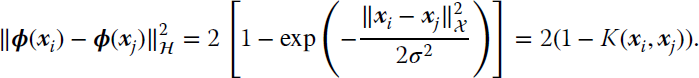
Note that the metric solely depends on the original data points yet computed implicitly in a higher dimensional feature space ![]() , whose notion of distance is controlled by the parameter σ: the larger σ is the smoother (linear) is the space. Actually,
, whose notion of distance is controlled by the parameter σ: the larger σ is the smoother (linear) is the space. Actually, ![]() reduces the RBF kernel to approximately compute the Euclidean distance between vectors, which reduces the metric tensor to gμν = 1.
reduces the RBF kernel to approximately compute the Euclidean distance between vectors, which reduces the metric tensor to gμν = 1.
Kernel Online Anomaly Detector
Let us imagine now that we receive incoming samples online. The problem now is to select the informative samples and discard the anomalous ones. This way the machine will not grow indefinitely and will retain only the information contained in the most useful incoming data points. Studying how rare a sample is becomes very complex with kernels because we do not have the inverse function from Hilbert space ![]() to input space to measure normality in physically meaningful units. Remember that, even though we never actually map samples to Hilbert spaces explicitly, the model and the metric are both defined therein. However, we can actually estimate distances in Hilbert spaces implicitly via reproducing kernels. For this, one only has to check if, given a previous set of N examples xi, a test incoming point x* is inside a sufficiently big ball of mean
to input space to measure normality in physically meaningful units. Remember that, even though we never actually map samples to Hilbert spaces explicitly, the model and the metric are both defined therein. However, we can actually estimate distances in Hilbert spaces implicitly via reproducing kernels. For this, one only has to check if, given a previous set of N examples xi, a test incoming point x* is inside a sufficiently big ball of mean ![]() :
:
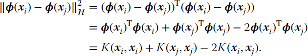
Note that one has to estimate distances to empirical means in Hilbert spaces. On the one hand, it is straightforward to show that we can compute distances between points using kernels, as before:
On the other hand, one can readily define the distance to the empirical mean in ![]() as
as ![]() , and we can compute it via kernels:
, and we can compute it via kernels:

Therefore, we only have to test the following condition over x* to check for largely anomalous points in Hilbert spaces:

Therefore, from an operational point of view, one only has to store a scalar ![]() accounting for the maximum similarity (minimum distance) among all the training samples, and then to check if the new example x* is beyond that threshold θ. This procedure is known as the KOAD, and has been successfully used in several applications, including the detection of anomalies in backbone routers communications (Ahmed et al., 2007).
accounting for the maximum similarity (minimum distance) among all the training samples, and then to check if the new example x* is beyond that threshold θ. This procedure is known as the KOAD, and has been successfully used in several applications, including the detection of anomalies in backbone routers communications (Ahmed et al., 2007).
Difference Kernels for Change Detection
We can use the previous property of kernels to define particular kernels for change detection. Let us now define a temporal classification scenario, in which we aim to detect the presence or absence of changes in the acquisition. This is a standard problem in surveillance applications and change detection from satellite imagery (Camps‐Valls et al., 2008). A standard, extremely simple technique is called the change vector analysis in which a threshold on the difference vector between two consecutive acquisitions t and t − 1 (i.e., d = xt − xt−1) is applied to detect changes. This difference vector can be formulated in the kernel feature space by defining a proper kernel mapping function:
We should note that the implementation is easy as it only involves application of kernel functions to define the differential metric among observations. Such a difference kernel can then be included in any supervised or unsupervised kernel classifier.3
11.2.2 Clustering in Feature Spaces
A complementary way to perform clustering in feature spaces is to follow the standard kernelization procedure. Let us introduce in this section the main concepts involved before defining the following kernel methods. Clustering methods try to obtain partitions of the data based on the optimization of a particular objective function, giving as result separation hypersurfaces among clusters. To handle nonlinearly separable clusters, the methods often define multiple centroids to provide a richer description of the dataset at hand.
Notationally, let us consider a set of data points ![]() so
so ![]() . The set of centroids
. The set of centroids ![]() for this dataset is called a codebook, and is defined as
for this dataset is called a codebook, and is defined as ![]() , with c ≪ N. Each element of
, with c ≪ N. Each element of ![]() ,
, ![]() , is called a centroid or codevector. Each centroid
, is called a centroid or codevector. Each centroid ![]() defines the so‐called Voronoi region
defines the so‐called Voronoi region ![]() as the set of vectors fulfilling the following condition (Aurenhammer, 1991):
as the set of vectors fulfilling the following condition (Aurenhammer, 1991): ![]() . Each Voronoi region is convex and its boundaries are linear segments. A further definition we need is the Voronoi set,
. Each Voronoi region is convex and its boundaries are linear segments. A further definition we need is the Voronoi set, ![]() , of the centroid
, of the centroid ![]() , being the subset of
, being the subset of ![]() for which the centroid
for which the centroid ![]() is the nearest vector; that is,
is the nearest vector; that is, ![]() . A partition of ℝd induced by all Voronoi regions is called a Voronoi tessellation or Dirichlet tessellation (Aurenhammer, 1991).
. A partition of ℝd induced by all Voronoi regions is called a Voronoi tessellation or Dirichlet tessellation (Aurenhammer, 1991).
Kernel k‐Means
Let us start by summarizing the formulation and optimization of the standard k‐means, and then we will show how to kernelize it. The goal of the canonical k‐means is to construct a Voronoi tessellation by moving k centroids to the arithmetic mean of their Voronoi sets. To achieve this, the k‐means algorithm searches the elements of ![]() that jointly minimize the empirical quantization error
that jointly minimize the empirical quantization error

which can be achieved if each centroid ![]() fulfills the centroid condition
fulfills the centroid condition

In the case of using the Euclidean distance, such a condition reduces to
where ![]() denotes the cardinality of
denotes the cardinality of ![]() . The k‐means algorithm is defined by the following steps: (1) choose the number k of clusters; (2) initialize
. The k‐means algorithm is defined by the following steps: (1) choose the number k of clusters; (2) initialize ![]() with a set of centroids
with a set of centroids ![]() randomly selected; (3) compute the Voronoi set
randomly selected; (3) compute the Voronoi set ![]() for each centroid
for each centroid ![]() ; (4) move each centroid
; (4) move each centroid ![]() to the mean of
to the mean of ![]() using Equation 11.11; and (5) stop the algorithm if no changes are observed, otherwise go to step 3. Note that the k‐means algorithm is an example of an EM algorithm. Step 3 is the expectation, and step 4 is the maximization. The convergence of the k‐means algorithm is guaranteed since each EM algorithm is always convergent to a local minimum (Bottou and Bengio, 1995).
using Equation 11.11; and (5) stop the algorithm if no changes are observed, otherwise go to step 3. Note that the k‐means algorithm is an example of an EM algorithm. Step 3 is the expectation, and step 4 is the maximization. The convergence of the k‐means algorithm is guaranteed since each EM algorithm is always convergent to a local minimum (Bottou and Bengio, 1995).
In order to obtain the kernel k‐means algorithm, we just translate the definitions and concepts before to a feature space. The first step is mapping our dataset ![]() to a high‐ dimensional feature space using a nonlinear map ϕ. The codebook is defined in the feature space as Vϕ = {ϕ(v1), …, ϕ(vk)}. We have a Voronoi region in the feature space defined by
to a high‐ dimensional feature space using a nonlinear map ϕ. The codebook is defined in the feature space as Vϕ = {ϕ(v1), …, ϕ(vk)}. We have a Voronoi region in the feature space defined by ![]() , and the Voronoi set
, and the Voronoi set ![]() of the centroid ϕ(
of the centroid ϕ(![]() ) defined as
) defined as ![]() . In this case, the Voronoi regions induce a Voronoi tessellation in the feature space.
. In this case, the Voronoi regions induce a Voronoi tessellation in the feature space.
The steps of the k‐means algorithm in the feature space are the same as the ones described in Section 11.2.1. The only difference is that the maximization step is computed using the following equation:

The problem is that we do not explicitly know ϕ and cannot move the centroid using Equation 11.12. This issue is solved using the representer theorem (Schölkopf and Smola, 2002), so that we can write each centroid in the feature space as a linear combination of the mapped data vectors, ![]() . By replacing the expansion into Equation 11.12, and noting that αij should be zero if
. By replacing the expansion into Equation 11.12, and noting that αij should be zero if ![]() , we obtain
, we obtain

which allows us to compute the closest feature space centroid for each sample, and update the coefficients αij accordingly. As in the standard k‐means algorithm, the procedure is repeated until all αij do not change significantly.
Kernel Fuzzy Clustering
Fuzzy clustering is essentially dealing with the elusive definition of hard and fuzzy partitions (Pal et al., 2005). Clustering solutions, such those offered by k‐means, do not offer disambiguation of cluster membership of samples that do not fit exactly to one single cluster but to several clusters in different degrees. Let us define a fuzzy‐c partition (or clustering) as

where the set ![]() can be defined with the membership matrix
U of size c × N, with 2 ≤ c < N and
can be defined with the membership matrix
U of size c × N, with 2 ≤ c < N and ![]() . Each element Uij is the membership of the jth pattern to the ith cluster, and the constraints ensure that (1) the sum of the membership of a pattern to all clusters is one (probabilistic constraint), and (2) a cluster cannot by empty or contain all samples.
. Each element Uij is the membership of the jth pattern to the ith cluster, and the constraints ensure that (1) the sum of the membership of a pattern to all clusters is one (probabilistic constraint), and (2) a cluster cannot by empty or contain all samples.
Now, given a codebook ![]() and a membership set
and a membership set ![]() , the fuzzy c‐means algorithm (Pal et al., 2005) minimizes the functional
, the fuzzy c‐means algorithm (Pal et al., 2005) minimizes the functional

subject to  , ∀j. The parameter m establishes the fuzziness of the membership. For m = 1 the classic k‐means hard clustering algorithm is obtained, whereas large values of m tend to set all memberships the same, and hence no structure is found on the data.
The functional in Equation 11.15 is minimized defining a Lagrangian function for each sample xj:

and deriving with respect to ![]() and Uij and setting to zero we obtain the following two equations:
and Uij and setting to zero we obtain the following two equations:

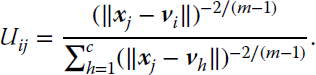
This pair of equations is used with a Picard iteration method (Pal et al., 2005) composed of two steps. In the first step, the membership variables Uij are kept fixed and the codevectors ![]() are optimized. Then, the second step optimizes the membership variables while the codevectors are fixed. These two steps are repeated until the variables change less than a predefined threshold. Equation 11.18 shows that the fuzzy membership of an input sample decreases as the distance increases. The sum in the denominator acts as a normalization factor.
are optimized. Then, the second step optimizes the membership variables while the codevectors are fixed. These two steps are repeated until the variables change less than a predefined threshold. Equation 11.18 shows that the fuzzy membership of an input sample decreases as the distance increases. The sum in the denominator acts as a normalization factor.
Next, we show two approaches to obtain a kernel version of the fuzzy clustering algorithm. One is based in the kernelization of the metric, and the other directly solves the equations of fuzzy c‐means in feature space.
Kernel Fuzzy Clustering Based on the Metric Kernelization
The functional to minimize is the same as in Equation 11.15 but in a high‐dimensional feature space:

subject to ![]() , ∀i. In order to minimize this cost function, we take derivatives with respect to vj and Uij. To be able to apply the kernel trick and obtain a practical solution, we explicitly compute the derivatives of the kernel function, which for the RBF kernel the result is as follows:
, ∀i. In order to minimize this cost function, we take derivatives with respect to vj and Uij. To be able to apply the kernel trick and obtain a practical solution, we explicitly compute the derivatives of the kernel function, which for the RBF kernel the result is as follows:

Computing all the derivatives and equating them to zero we obtain the following equations for the Picard iteration method:


which are now solely based on evaluating kernel functions, and hence the method can be easily implemented.
Kernel Fuzzy Clustering in Feature Space
The functional to minimize is shown in Equation 11.19. Instead of obtaining a solution taking derivatives using ![]() and Uij, now we use the representer theorem to express ϕ(
and Uij, now we use the representer theorem to express ϕ(![]() ) as a linear combination of samples in feature space; that is,
) as a linear combination of samples in feature space; that is, ![]() . This will allow us to compute the distance appearing in Equation 11.19 just in terms of the kernel function as in Equation 11.1. Therefore, let us rewrite the functional as
. This will allow us to compute the distance appearing in Equation 11.19 just in terms of the kernel function as in Equation 11.1. Therefore, let us rewrite the functional as

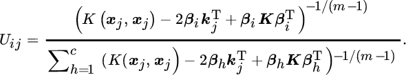
where kj is the jth row of the kernel; that is, kj := [K(xj, x1), …, K(xj, xN)]T, and β = [β1, …, βN] are the weights for the ϕ(v) codevector, and K is the whole kernel matrix. This functional can be derived with respect to the variables βi and Uij, obtaining the equations we need for the Picard iteration method:

There is an alternative pair of equivalent equations that we can obtain using the following reasoning. Deriving the functional in Equation 11.19 directly with respect to ϕ(![]() ) we will obtain, similarly to Equation 11.17, the expansion
) we will obtain, similarly to Equation 11.17, the expansion

where we have defined ai as

With Equations 11.26 and 11.25 we can rewrite Equation 11.24 as

where ui := [(ui1)m, …, (uin)m]T. It is clear that Equations 11.24 and 11.27 are equivalent, noting that, by definition, ![]() . However, the Picard iteration method is easier to implement using Equations 11.26 and 11.27.
. However, the Picard iteration method is easier to implement using Equations 11.26 and 11.27.
Kernel Self‐Organizing Maps
A self‐organized map (SOM) (Kohonen, 1990) is a type of artificial NN trained to obtain a low‐dimensional (most of the times 2D) representation of the input data. The training phase is unsupervised where SOM defines a function that tries to preserve the topological properties of the input dataset. SOMs are typically used to obtain low‐dimensional visualizations of high‐dimensional data. As for other NNs, an SOM consists of a series of interconnected nodes or neurons. Each node has a weight vector of the same dimension as the input data samples, and a location in the map space, while each vector of the input space is placed on the map space by finding the closest/nearest node in the map space.
Let us define our coodebook, denoted ![]() , as the set of neurons (centroids) that will compose the map. The first step of the training phase is to randomly select the weights of the neurons in
, as the set of neurons (centroids) that will compose the map. The first step of the training phase is to randomly select the weights of the neurons in ![]() . Alternatively, Kohonen (1990) showed that it is possible to speed up the training phase by evenly sampling the subspace spanned by the two largest principal component eigenvectors, instead of randomly selecting the first neurons’ weights. The second step is to take an input sample x from
. Alternatively, Kohonen (1990) showed that it is possible to speed up the training phase by evenly sampling the subspace spanned by the two largest principal component eigenvectors, instead of randomly selecting the first neurons’ weights. The second step is to take an input sample x from ![]() and obtain the nearest neuron using a distance function d (Euclidean of Manhattan distances are the most often used). The shortest distance would be the one that solves
and obtain the nearest neuron using a distance function d (Euclidean of Manhattan distances are the most often used). The shortest distance would be the one that solves ![]() . Then the weights of the neurons are adapted using a standard gradient descent strategy:
. Then the weights of the neurons are adapted using a standard gradient descent strategy:
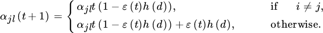
where h is a decreasing function of the distance d; for example, ![]() . Here, σ(t) is a decreasing function of t,
. Here, σ(t) is a decreasing function of t, ![]() , ε(t) is also a decreasing function of t,
, ε(t) is also a decreasing function of t, ![]() , and where the subscripts “i” and “f” indicate the initial and final values respectively. The adaptation of neurons vj in Equation 11.28 is repeated until a predefined number of iterations is achieved; that is, t = tmax.
, and where the subscripts “i” and “f” indicate the initial and final values respectively. The adaptation of neurons vj in Equation 11.28 is repeated until a predefined number of iterations is achieved; that is, t = tmax.
In order to reformulate the SOM in the feature space, we need to first define our set of initial neurons ϕ(vj). Since we do not know ϕ explicitly, we use the representer theorem to write each neuron as a combination of mapped input samples:
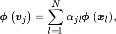
and we randomly initialize the coefficients αjl. Then, given an input sample ϕ(xi), we need to compute the nearest neuron to it:

which, after applying the kernel trick, translates into
Finally, the neurons in the feature space are updated as
which according to Equation 11.29 can be expressed as

from which we can now obtain the update rule for αjl as follows:
Note that the updating rule can be obtained iteratively until convergence.
11.3 Domain Description Via Support Vectors
As an alternative to the previous approaches for clustering with kernels, the description of the domain can be done via support vectors. Instead of directly kernelizing the metric or the clustering algorithm, one attempts here to describe the data distribution in feature spaces with a minimum volume hypersphere enclosing all data points but the outliers, which translates into a hypersurface in the original input space. This idea leads to several algorithms, such as the one‐class SVM (OC‐SVM) and the related support vector domain description (SVDD). After computing the ball with these methods, the SVC method permits one to assign labels to patterns in input space enclosed by the same surface. In the next subsections we will review the formulation of these three main approaches.
11.3.1 Support Vector Domain Description
A different problem statement for classification is given by the SVDD (Tax and Duin, 1999). The SVDD is a method to solve one‐class problems, where one tries to describe one class of objects, distinguishing them from all other possible objects.
The problem notation is defined as follows. Let ![]() be a dataset belonging to a given class of interest. The purpose is to find a minimum volume hypersphere in a high‐dimensional feature space
be a dataset belonging to a given class of interest. The purpose is to find a minimum volume hypersphere in a high‐dimensional feature space ![]() , with radius R > 0 and center
, with radius R > 0 and center ![]() , which contains most of these data objects (Figure 11.1a). Since the training set may contain outliers, a set of slack variables ξi ≥ 0 is introduced, and the problem becomes
, which contains most of these data objects (Figure 11.1a). Since the training set may contain outliers, a set of slack variables ξi ≥ 0 is introduced, and the problem becomes

constrained to
where parameter C controls the trade‐off between the volume of the hypersphere and the permitted errors. Parameter ν, defined as ν = 1/(NC), can be used as a rejection fraction parameter to be tuned, as noted by Schölkopf et al. (1999).

Figure 11.1 Illustration of the one‐class kernel classifiers. (a) In the SVDD, the hypersphere containing the target data is described by center a and radius R, and samples in the boundary and outside the ball are unbounded and bounded support vectors, respectively. (b) In the case of the OC‐SVM, all samples from the target class are mapped with maximum distance to the origin.
The dual functional is a QP problem that yields a set of Lagrange multipliers (αi) corresponding to constraints in Equation 11.35. When free parameter C is adjusted properly, most of the αi are zero, giving a sparse solution. The Lagrange multipliers are also used to calculate the distance from a test point to the center R(x*):
which is compared with ratio R. Unbounded support vectors are those samples xi satisfying ![]() , while bounded support vectors are samples whose associated αi = C, which are considered outliers.
, while bounded support vectors are samples whose associated αi = C, which are considered outliers.
11.3.2 One‐Class Support Vector Machine
In the OC‐SVM, instead of defining a hypersphere containing all examples, a hyperplane that separates the data objects from the origin with maximum margin is defined (Figure 11.1b). It can be shown that, when working with normalized data and the RBF Gaussian kernel, both methods yield the same solution (Schölkopf et al., 1999).
Notationally, in the OC‐SVM, we want to find a hyperplane w which separates samples xi from the origin with margin ρ. The problem thus becomes

constrained to
The problem is solved through its Lagrangian dual introducing a set of Lagrange multipliers αi. The margin ρ can be computed as ![]() .
.
11.3.3 Relationship Between Support Vector Domain Description and Density Estimation
Let us now point out the connection between pdf estimation and the previous one‐class kernel classifiers. The goal of kernel density estimation (KDE) is to estimate the unknown pdf p(x) given N i.i.d. samples {x1, …, xN} drawn from it. The kernel (Parzen) estimate of the pdf using an arbitrary kernel function Kσ(⋅) parameterized with a length‐scale parameter σ is given by

where K is typically a Gaussian kernel, and the hyperparameters of the model (e.g., the length scale or kernel width) can be obtained via ML estimation or fixed through ad hoc rule of thumb rules, such as Silverman’s rule. Other kernel functions can be used: uniform, normal, triangular, bi‐weighted, tri‐weighted, just to name a few. The Epanechnikov kernel, for example, is optimal in an MSE sense. The interested reader can explore the MATLAB function ksdensity.m and the MATLAB KDE toolbox available oin the book’s web page.
Density estimates can be used to characterize distributions and to design anomaly detection schemes. Note, for instance, that once ![]() is obtained, an anomaly detector can be readily defined simply as
is obtained, an anomaly detector can be readily defined simply as
Now, by plugging the previous Gaussian kernel estimate in here and defining a centroid in the feature space as the mean of the mapped samples, a KDE‐based anomaly detector can be readily derived by simply kernelizing the distance between a test point x* and all the training points (see Section 11.2.1):

Note that definition of SVDD seen previously in Equations 11.34 and 11.35 leads to an SVDD anomaly detector in the form
where αi > 0 are support vectors. Comparing Equation 11.43 with Equation 11.44 we see they are very similar, except that the SVDD anomaly detector places unequal weights on the training points xi. In other words, while the kernel KDE works as an unsupervised method where the centroid is placed at  , the SVDD is a supervised method that uses training (labeled) samples to place the centroid at
  . Figure 11.2 shows a toy example comparing the boundaries obtained by the SVDD (centroid at a) and KDE (centroid at μϕ).

Figure 11.2 Boundary comparison between SVDD (sphere centered at a) and KDE (sphere centered at μϕ).
11.3.4 Semi‐supervised One‐Class Classification
Exploiting unlabeled information in one‐class classifiers can be done via semi‐supervised versions of the OC‐SVM. A particularly convenient instantiation is the biased‐SVM (b‐SVM) classifier, which was originally proposed by Liu et al. (2003) for text classification using only target and unlabeled data. The underlying idea of the method lies on the assumption that if the sample size is large enough, minimizing the number of unlabeled samples classified as targets while correctly classifying the labeled target samples will give an accurate classifier.
Let us consider again the dataset ![]() made up of l labeled samples and u unlabeled samples (N = l + u). The l labeled samples all belong to the same class: the target class. Concerning unlabeled samples, they are treated by the algorithm as being all outliers, although their class is unknown. This characteristic makes b‐SVM a sort of semi‐supervised classifier. Under these assumptions, the b‐SVM formulation is defined as
made up of l labeled samples and u unlabeled samples (N = l + u). The l labeled samples all belong to the same class: the target class. Concerning unlabeled samples, they are treated by the algorithm as being all outliers, although their class is unknown. This characteristic makes b‐SVM a sort of semi‐supervised classifier. Under these assumptions, the b‐SVM formulation is defined as
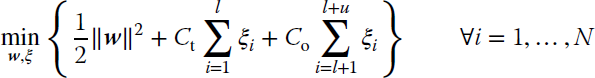
subject to
where ξi ≥ 0 are slack variables, and Ct and Co are the costs assigned to errors on target and outlier (unlabeled) classes, respectively. The two cost values should be adjusted to fulfill the goal of classifying the target class correctly while at the same time trying to minimize the number of unlabeled samples classified as target class. To achieve this goal, Ct should have a large value, as initially we trust our labeled training set, and Co a small value, because it is unknown whether the samples unlabeled are actually targets or outliers.
11.4 Kernel Matched Subspace Detectors
Target detection from data is of great interest in many applications. Detecting targets is typically described as a two‐step methodology: first, a specific detector identifies anomalies; second, a classifier is aimed at identifying whether the anomaly is a target or natural clutter. In many application domains, this step is only possible if the target signature is known, which can be obtained from a library of “pure elements” or learned from data by using subspace matched filters. Several techniques have been proposed in the literature, such as the Reed–Xiaoli anomaly detector (Reed and Yu, 1990), the orthogonal subspace projection (OSP) (Harsanyi and Chang, 1994), the Gaussian mixture model (GMM) (Stein et al., 2002), the cluster‐based detector (Stein et al., 2002), or the signal subspace processor (Ranney and Soumekh, 2006). In recent years, many detection algorithms based on spectral matched (subspace) filters have been reformulated under the kernel methods framework: matched subspace detector, orthogonal subspace detector, as well as adaptive subspace detectors (Kwon and Nasrabadi, 2005a). Certainly, the use of kernel methods alleviates several key problems and offers many advantages: they combat the high‐dimensionality problem, make the method robust to noise, and allow for flexible nonlinear mappings with controlled (regularized) complexity (Shawe‐Taylor and Cristianini, 2004).
This section deals with target/anomaly detection and its corresponding kernelized extensions under the viewpoint of matched subspace detectors. This topic has been very active in the last decade, and also in the particular field of signal and image anomaly detection. We pay attention to different kernel anomaly subspace detectors: KOSP, KSAM and the family of KACD that generalizes several anomaly detectors under Gaussian and EC distributions.
11.4.1 Kernel Orthogonal Subspace Projection
The OSP algorithm (Harsanyi and Chang, 1994) tries to maximize the SNR in the subspace orthogonal to the background subspace. OSP has been widely adopted in the community of automatic target recognition because of its simplicity (only depends on the noise second‐order statistics) and its good behavior. In the standard formulation of the OSP algorithm (Harsanyi and Chang, 1994), a linear mixing model is assumed for each d‐dimensional observed point r as follows:
where M is the matrix of size (d × p) containing the p endmembers (i.e., pure constituents of the observed mixture) contributing to the mixed point r, ![]() contains the weights in the mixture (sometimes called abundance vector), and
contains the weights in the mixture (sometimes called abundance vector), and ![]() stands for an additive zero‐mean Gaussian noise vector. In order to identify a particular desired point d in a data set (e.g., a pixel in an image) with corresponding abundance αp, the earlier expression can be organized by rewriting the M matrix in two submatrices M = [U|d] and α = [γ, αp]T, so that
stands for an additive zero‐mean Gaussian noise vector. In order to identify a particular desired point d in a data set (e.g., a pixel in an image) with corresponding abundance αp, the earlier expression can be organized by rewriting the M matrix in two submatrices M = [U|d] and α = [γ, αp]T, so that
where the columns of U represent the undesired points and γ contains their abundances. The OSP operator that maximizes the SNR performs two steps. First, an annihilating operator rejects the background points so that only the desired point should remain in the data subspace. This operator is given by the (d × d) matrix ![]() , where U† is the right Moore–Penrose pseudoinverse of U. The second step of the OSP algorithm is represented by the filter w that maximizes the SNR of the filter output; that is, the matched filter w = kd, where k is an arbitrary constant (Harsanyi and Chang, 1994; Kwon and Nasrabadi, 2005b). The OSP detector is given by
, where U† is the right Moore–Penrose pseudoinverse of U. The second step of the OSP algorithm is represented by the filter w that maximizes the SNR of the filter output; that is, the matched filter w = kd, where k is an arbitrary constant (Harsanyi and Chang, 1994; Kwon and Nasrabadi, 2005b). The OSP detector is given by ![]() = dT
= dT![]() r, and the output of the OSP classifier is
r, and the output of the OSP classifier is
By using the singular‐value decomposition of U = BΣAT, where B is the eigenvector of UUT = BΣΣTBT and A is the eigenvector of UTU = AΣTΣA. The annihilating projector operator becomes ![]() , where the columns of B are obtained from the eigenvectors of the covariance matrix of the background samples. This finally yields the expression
, where the columns of B are obtained from the eigenvectors of the covariance matrix of the background samples. This finally yields the expression
Figure 11.3 shows the effect of the OSP algorithm on a toy data set.

Figure 11.3 The standard (linear) OSP method first performs a linear transformation that looks for projections that identify the subspace spanned by the background, and then the background suppression is carried out by projecting the data onto the subspace orthogonal to the one spanned by the background components. The kernel version of this algorithm consists of the same procedure yet performed in the kernel feature space.
A nonlinear kernel‐based version of the OSP algorithm can be devised by defining a linear OSP in an appropriate Hilbert feature space where samples are mapped to through a kernel mapping function ϕ(⋅). Similar to the previous linear case, let us define the annihilating operator now in the feature space as ![]() = Iϕ − Bϕ
= Iϕ − Bϕ![]() . Then, the output of the OSP classifier in the feature space is now trivially given by
. Then, the output of the OSP classifier in the feature space is now trivially given by
The columns of matrix Bϕ (e.g., denoted as bϕj) are the eigenvectors of the covariance matrix of the undesired background signatures. Clearly, each eigenvector in the feature space can be expressed as a linear combination of the input vectors in the feature space transformed through the function ϕ(⋅). Hence, one can write bϕj = Φbβj – where Φb contains the mapped background points Xb, and βj are the eigenvectors of the (centered) Gram matrix ![]() , whose entries are Kbb(bi, bj) = ϕ(bi)Tϕ(bj), and bi are background points.4 The kernelized version in Equation 11.50 is given (Kwon and Nasrabadi, 2005b) by
, whose entries are Kbb(bi, bj) = ϕ(bi)Tϕ(bj), and bi are background points.4 The kernelized version in Equation 11.50 is given (Kwon and Nasrabadi, 2005b) by
where k are column vectors referred to as the empirical kernel maps and the subscripts indicate the elements entering the corresponding kernel function: d for the desired target, r the observed point, and subscript m indicates the concatenation of both; that is, Xm = [Xb|d]. Also ![]() is the matrix containing the eigenvectors βj described earlier; and ? is the matrix containing the eigenvectors υj, similar to βj yet obtained from the centered kernel matrix Km, m thus working with the expanded matrix Xm. Listing 11.1 illustrates the simplicity of the code for the KOSP method.
is the matrix containing the eigenvectors βj described earlier; and ? is the matrix containing the eigenvectors υj, similar to βj yet obtained from the centered kernel matrix Km, m thus working with the expanded matrix Xm. Listing 11.1 illustrates the simplicity of the code for the KOSP method.
11.4.2 Kernel Spectral Angle Mapper
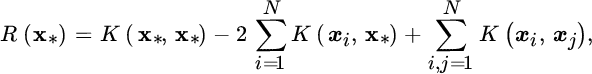
The spectral angle mapper (SAM) is a method for directly comparing image spectra (Kruse et al., 1993). Since its seminal introduction, SAM has been widely used in chemometrics, astrophysics, imaging, hyperspectral image analysis, industrial engineering, and computer vision applications (Ball and Bruce 2007; Cho et al. 2010; García‐Allende et al. 2008; Hecker et al. 2008), just to name a few. The measure achieved widespread popularity thanks to its implementation in software packages, such as ENVI or ArcGIS. The reason is simple: SAM is invariant to (unknown) multiplicative scalings of spectra due to differences in illumination and angular orientation (Keshava, 2004). SAM is widely used for fast spectral classification, as well as to evaluate the quality of extracted endmembers, and the spectral quality of an image compression algorithm.
The popularity of SAM is mainly due to its simplicity and geometrical interpretability. However, the main limitation of the measure is that it only considers second‐order angle dependencies between spectra. In the following, we will see how to generalize the SAM measure to the nonlinear case by means of kernels (Camps‐Valls and Bruzzone, 2009). This short note aims to characterize KSAM theoretically, and to show its practical convenience over the widespread linear counterpart. KSAM is very easy to compute, and can be used in any kernel machine. KSAM also inherits all properties of the original distance, is a valid reproducing kernel, and is universal. The induced metric by the kernel will be easily derived by traditional tensor analysis, and tuning the kernel hyperparameter of the squared exponential kernel function used is shown to be stable. KSAM is tested here in a target detection scenario for illustration purposes. The spatially explicit detection and metric maps give us useful information for semiautomatic anomaly/target detection.
Given two d‐dimensional samples, ![]() , the SAM measures the angle θ between them:
, the SAM measures the angle θ between them:

KSAM requires the definition of a feature mapping ϕ(⋅) to a Hilbert space ![]() endorsed with the kernel reproducing property. Now, if we simply map the original data to
endorsed with the kernel reproducing property. Now, if we simply map the original data to ![]() with a mapping
with a mapping ![]() , the SAM can be expressed in
, the SAM can be expressed in ![]() as
as
Having access to the coordinates of the new mapped data is not possible unless one explicitly defines the mapping function ϕ. It is possible to compute the new measure implicitly via kernels:
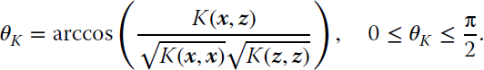
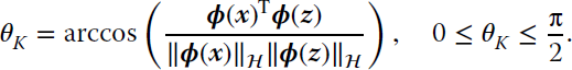
Popular examples of reproducing kernels are the linear kernel K(x, z) = xTz, the polynomial K(x, z) = (xTz + 1)d, and the RBF kernel ![]() . In the linear kernel, the associated RKHS is the space ℝd itself and KSAM reduces to the standard linear SAM. In polynomial kernels of degree d, KSAM effectively only compares moments up to order d. For the Gaussian kernel, the RKHS is of infinite dimension and KSAM measures higher order feature dependences. In addition, note that for RBF kernels, self‐similarity K(x, x) = 1, and thus the measure simply reduces to
. In the linear kernel, the associated RKHS is the space ℝd itself and KSAM reduces to the standard linear SAM. In polynomial kernels of degree d, KSAM effectively only compares moments up to order d. For the Gaussian kernel, the RKHS is of infinite dimension and KSAM measures higher order feature dependences. In addition, note that for RBF kernels, self‐similarity K(x, x) = 1, and thus the measure simply reduces to ![]() , 0 ≤ θK ≤ π/2. Following the code in Listing 11.1, we show a simple (just one line) snippet of KSAM in Listing 11.2.
, 0 ≤ θK ≤ π/2. Following the code in Listing 11.1, we show a simple (just one line) snippet of KSAM in Listing 11.2.
11.5 Kernel Anomaly Change Detection
Anomalous change detection (ACD) differs from standard change detection in that the goal is to find anomalous or rare changes that occurred between two datasets. The distinction is important both statistically and from the practitioner’s point of view. Statistically speaking, standard change detection emphasizes all the differences between the two data distributions, while ACD is more interested in modeling accurately the tails of the difference distribution.
The interest in ACD is vast, and many methods have been proposed in the literature, ranging from regression‐based approaches like in the chronocrome (Schaum and Stocker, 1997), where big residuals are associated with anomalies, to equalization‐based approaches that rely on whitening principles (Mayer et al., 2003), as well as multivariate methods (Arenas‐García et al., 2013) that reinforce directions in feature spaces associated with noisy or rare events (Green et al., 1998; Nielsen et al., 1998). Theiler and Perkins (2006) formalized the main differences between the two fields and introduced a framework for ACD. The framework assumes data Gaussianity, yet the derived detector delineates hyperbolic decision functions. Even though the Gaussian assumption reports some advantages (e.g., problem tractability and generally good performance) it is still an ad hoc assumption that it is not necessarily fulfilled in practice. This is the motivation in Theiler et al. (2010), where the authors introduce EC distributions that generalize the Gaussian distribution and prove more appropriate to modeling fatter tail distributions and thus detect anomalies more effectively. The EC decision functions are pointwise nonlinear and still rely on second‐order feature relations. In this section we will see the extension of the methods in Theiler et al. (2010) to cope with higher order feature relations through the theory of reproducing kernels.
11.5.1 Linear Anomaly Change Detection Algorithms
A family of linear ACD can be framed using solely cross‐covariance matrices, as illustrated in Theiler et al. (2010). Notationally, given two samples ![]() , the decision of anomalousness is given by
, the decision of anomalousness is given by
where ![]() ,
, ![]() , and
, and ![]() ,
, ![]() , and Cz = ZTZ, Cx = XTX, and Cy = YTY are the estimated covariance matrices with the available data. Parameters βx, βy ∈{0, 1} and the different combinations give rise to different anomaly detectors (see Table 11.1). These methods and some variants have been widely used in image analysis settings because of their simplicity and generally good performance (Chang and Lin 2002; Kwon et al. 2003; Reed and Yu 1990).
, and Cz = ZTZ, Cx = XTX, and Cy = YTY are the estimated covariance matrices with the available data. Parameters βx, βy ∈{0, 1} and the different combinations give rise to different anomaly detectors (see Table 11.1). These methods and some variants have been widely used in image analysis settings because of their simplicity and generally good performance (Chang and Lin 2002; Kwon et al. 2003; Reed and Yu 1990).
Table 11.1 A family of ACD algorithms (HACD: hyperbolic ACD).
| ACD algorithm | βx | βy |
| RX | 0 | 0 |
| Chronocrome y|x | 0 | 1 |
| Chronocrome x|y | 1 | 0 |
| HACD | 1 | 1 |
However, these methods are hampered by a fundamental problem: the assumption of Gaussianity that is implicit in the formulation. Accommodating other data distributions may not be easy in general. Theiler et al. (2010) introduced an alternative ACD to cope with EC distributions (Cambanis et al., 1981): roughly speaking, the idea is to model the data using the multivariate Student distribution. The formulation introduced in (Theiler et al., 2010) gives rise to the following decision of EC anomalousness:

where ν controls the shape of the generalized Gaussian: for ![]() the solution approximates the Gaussian and for ν → 2 it diverges.
the solution approximates the Gaussian and for ν → 2 it diverges.
11.5.2 Kernel Anomaly Change Detection Algorithms
Note that the previous methods solely depend on estimating covariance matrices with the available data, and use them as a metric for testing. The methods are fast to apply, delineate pointwise nonlinear decision boundaries, but still rely on second‐order statistics. We solve the issue as usual using reproducing kernel functions.
For the sake of simplicity, we just show how to estimate the anomaly term ξx in the Hilbert space, ![]() . The other terms are derived in the same way. Notationally, let us map all the observations to a higher dimensional Hilbert feature space
. The other terms are derived in the same way. Notationally, let us map all the observations to a higher dimensional Hilbert feature space ![]() by means of the feature map ϕ : x → ϕ(x). The mapped training data matrix
by means of the feature map ϕ : x → ϕ(x). The mapped training data matrix ![]() is now denoted as
is now denoted as ![]() . Note that one could think of different mappings: ϕ : x → ϕ(x) and ψ : y → ψ(y). However, in our case, we are forced to consider mapping to the same Hilbert space because we have to stack the mapped vectors to estimate ξz; that is,
. Note that one could think of different mappings: ϕ : x → ϕ(x) and ψ : y → ψ(y). However, in our case, we are forced to consider mapping to the same Hilbert space because we have to stack the mapped vectors to estimate ξz; that is, ![]() . The mapped training data to Hilbert spaces are denoted as
. The mapped training data to Hilbert spaces are denoted as ![]() respectively. In order to estimate
respectively. In order to estimate ![]() for a test example x*, we first map the test point ϕ(x*) and then apply
for a test example x*, we first map the test point ϕ(x*) and then apply
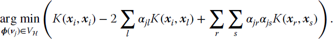
Note that we do not have access to either the samples in the feature space or the covariance. We can, nevertheless, estimate the eigendecomposition of the covariance matrix in kernel feature space; that is, ![]() , where Λℋ is a diagonal matrix containing the eigenvalues and Vℋ contains the eigenvectors in columns. It is worth noting that the maximum number of eigenvectors equals the number of examples used N. Plugging the eigendecomposition of the covariance pseudoinverse
, where Λℋ is a diagonal matrix containing the eigenvalues and Vℋ contains the eigenvectors in columns. It is worth noting that the maximum number of eigenvectors equals the number of examples used N. Plugging the eigendecomposition of the covariance pseudoinverse ![]() , and after some linear algebra, one can express the term as
, and after some linear algebra, one can express the term as
We can replace all dot products by reproducing kernel functions using the representer theorem (Kimeldorf and Wahba, 1971; Shawe‐Taylor and Cristianini, 2004), and hence ![]() , where
, where ![]() contains the similarities between x* and all training points X; that is, k* := [K(x*, x1), …, K(x*, xN)]T, and
contains the similarities between x* and all training points X; that is, k* := [K(x*, x1), …, K(x*, xN)]T, and ![]() stands for the kernel matrix containing all training data similarities. The solution may need extra regularization
stands for the kernel matrix containing all training data similarities. The solution may need extra regularization ![]() ,
, ![]() . Therefore, in the kernel case, the decision of anomalousness is given by
. Therefore, in the kernel case, the decision of anomalousness is given by
where now ![]() ,
, ![]() , and
, and ![]() .
.
Equivalently, including these expressions in Equation 11.55, one obtains the EC kernel versions ![]() :
:

In the case of βx = βy = 0, the algorithm reduces to kernel RX which was introduced in Kwon and Nasrabadi (2005c). As in the linear case, one has to center the data before computing either covariance or Gram (kernel) matrices. This is done via the kernel matrix operation ![]() , where Hij = δij − (1/n), and δ represents the Kronecker delta δi, j = 1 if i = j and zero otherwise.
, where Hij = δij − (1/n), and δ represents the Kronecker delta δi, j = 1 if i = j and zero otherwise.
Two parameters need to be tuned in the kernel versions: the regularization parameter λ and the kernel parameter σ. In the examples, we will use two different isotropic kernel functions, ![]() : the standard Gaussian kernel dij = ∥xi − xj∥, and the SAM kernel
: the standard Gaussian kernel dij = ∥xi − xj∥, and the SAM kernel ![]() . We should note that, when a linear kernel is used,
. We should note that, when a linear kernel is used, ![]() , the proposed algorithms reduce to the linear counterparts proposed in Theiler et al. (2010). Working in the dual (or Q‐mode) with the linear kernel instead of the original linear versions can be advantageous only in the case of higher dimensionality than available samples, d > N.
, the proposed algorithms reduce to the linear counterparts proposed in Theiler et al. (2010). Working in the dual (or Q‐mode) with the linear kernel instead of the original linear versions can be advantageous only in the case of higher dimensionality than available samples, d > N.
11.6 Hypothesis Testing with Kernels
Statistical hypothesis testing plays a crucial role in statistical inference. After all, the core of science and engineering is about testing hypotheses,5 and in machine learning we do it through data analysis. Testing hypotheses is concurrently one of the key topics in statistical signal processing as well (Kay, 1993). A plethora of examples exists: from testing for equality of observations as in speaker verification (Bimbot et al., 2004; Rabiner and Schafer, 2007), to assessing statistical differences between data acquisitions, such as in change‐detection analysis (Basseville and Nikiforov, 1993) as seen before. Testing for a change‐point in a time series is also an important problem in DSP (Fearnhead, 2006), such as in monitoring applications involving biomedical or geoscience time series.
Very often we aim to compare two real datasets, or a real dataset with a synthetically generated one by a model that encodes the system’s governing equations. The result of such a test will tell us about the plausibility and the origin of the observations. In both cases, we need a solid measure to test the significance of their statistical difference, compared with an idealized null hypothesis in which no relationship is assumed (Kay, 1993). Hypothesis tests are used in determining what outcomes of a study would lead to a rejection of the null hypothesis for a prespecified level of significance. Imagine, presented with two datasets, we are interested in testing whether the underlying distributions are statistically different or not in the mean. Essentially, we have to test between two competing hypotheses, and decide upon them:
The hypothesis H0 is referred to as the null hypothesis, and HA is the alternative hypothesis. The process of distinguishing between the null hypothesis and the alternative hypothesis is aided by identifying two conceptually different types of errors (type I and type II), and by specifying parametric limits on, for example, how much type I error could be allowed. If the detector decides HA but H0 is true, we commit a type I error (also known as the false‐alarm rate), whereas if we decide H0 but HA is true, we make a type II error (also known as the missed‐detection rate).
Classical approaches to statistical hypothesis testing and detection (of changes and differences between samples) are parametric in nature (Basseville and Nikiforov, 1993). Procedures such as the CUSUM statistic6 or Hotelling’s T‐squared test assume that the data is Gaussian, whereas the χ2 and mutual information statistics can only be applied in finite‐valued data. These test statistics are widely used due to their simplicity and good results in general when the assumptions about the underlying distributions are fulfilled. Alternatively, non‐parametric hypothesis testing allows more robust and reliable results over larger classes of data distributions as this does not assume any particular form. Recently, nonparametric kernel‐based methods have appeared in the literature (Harchaoui et al., 2013).
In recent years, several kernel‐based hypothesis testing methods have been introduced. For a recent sound review, the reader is addressed to Harchaoui et al. (2013). We next review some of these methods under the framework of distribution embeddings and the concepts of mean elements and covariance operators (Eric et al. 2008; Fukumizu et al. 2007). These test statistics rely on the eigenvector basis of particular covariance operators and, under the alternative hypothesis, the tests correspond to consistent estimators of well‐known information divergences between probability distributions (Cover and Thomas, 2006). We give two instantiations of kernel hypothesis tests in dependence estimation and anomaly detection, while Chapter 12 will pay attention to a broader family of these kernel dependence measures for feature extraction.
11.6.1 Distribution Embeddings
Recall that our current motivation is to test statistical differences between distributions with kernels. Therefore, it is natural to ask ourselves about which are the appropriate descriptors of distributions embedded into possibly infinite‐dimensional Hilbert spaces. The distributions’ components therein can be described by the so‐called covariance operators and mean elements (Eric et al. 2008; Fukumizu et al. 2007; Harchaoui et al. 2013; Vakhania et al. 1987).
Notationally, let us consider a random variable x taking values in ![]() and a probability distribution ℙ. The mean element μℙ associated with x is the unique element of the RKHS
and a probability distribution ℙ. The mean element μℙ associated with x is the unique element of the RKHS ![]() , such that, for all
, such that, for all ![]() , we obtain
, we obtain
and the covariance operator
![]() attached to x fulfills
attached to x fulfills
In the empirical case, we are given a set of i.i.d. samples {x1, …, xN} drawn from ℙ, so we have to replace the previous population statistics by their empirical approximations to obtain the empirical mean ![]()

and the empirical covariance operator ![]() :
:

Interestingly, it can be shown that, for a large class of kernels, an embedding function m(⋅) that maps data into the kernel feature mean is injective (Harchaoui et al., 2013). Now, if we consider two probability distributions ℙ and ℚ on ![]() , and for all
, and for all ![]() the equality
the equality ![]() holds, then
holds, then ![]() for dense kernel functions K. This property has been exploited to define independence tests and hypothesis testing methods based on kernels, since it ensures that two distributions have the same RKHS mean iff they are the same, as we will see in Chapter 12.
for dense kernel functions K. This property has been exploited to define independence tests and hypothesis testing methods based on kernels, since it ensures that two distributions have the same RKHS mean iff they are the same, as we will see in Chapter 12.
11.6.2 Maximum Mean Discrepancy
Among several hypothesis testing algorithms, such as the kernel Fisher discriminant analysis and the kernel density‐ratio test statistic revised in Harchaoui et al. (2013), a simple and effective one is the maximum mean discrepancy (MMD) statistic. Gretton et al. (2005b) introduced the MMD statistic for comparing the means of two samples in kernel feature spaces; see Figure 11.11. Notationally, we are given samples ![]() from a so‐called source distribution, ℙx, and
from a so‐called source distribution, ℙx, and ![]() samples drawn from a second target distribution, ℙy. MMD reduces to estimate the distance between the two sample means in an RKHS
samples drawn from a second target distribution, ℙy. MMD reduces to estimate the distance between the two sample means in an RKHS ![]() where data are embedded:
where data are embedded:

This estimate can be shown to be equivalent to
where

and Lij = 1/N2 if xi and xj belong to the source domain, ![]() if xi and xj belong to the target domain, and Lij = −1/(NM) if xi and xj belong to the cross‐domain. MMD tends asymptotically to zero when the two distributions ℙx and ℙy are the same.
if xi and xj belong to the target domain, and Lij = −1/(NM) if xi and xj belong to the cross‐domain. MMD tends asymptotically to zero when the two distributions ℙx and ℙy are the same.
It is worth mentioning that MMD was concurrently introduced in the field of signal processing under the formalism of information‐theoretic learning (Principe, 2010). In such a framework, it can be shown that MMD corresponds to a Euclidean divergence. This can be shown easily. Let us assume two distributions p(x) and q(x) with N1 and N2 samples. The Euclidean divergence between them can be computed by exploiting the relation to the quadratic Rényi entropies (see Chapter 2 of Principe (2010)):

where G(⋅) denotes Gaussian kernels with standard deviation σ. This divergence reduces to compute the norm of the difference between the means in feature spaces:
which is equivalent to the MMD estimate introduced from the theory of covariance operators in Gretton et al. (2005b).
11.6.3 One‐Class Support Measure Machine
Let us give now an example of a kernel method for anomaly detection based on RKHS embeddings. A field of anomaly detection that has captured the attention recently is the so‐called grouped anomaly detection. The interest here is that the anomalies often appear not only in the data themselves, but also as a result of their interactions. Therefore, instead of looking for pointwise anomalies, here one is interested in groupwise anomalies. A recent method, based on SVC, was been introduced by Muandet and Schölkopf (2013). An anomalous group could be defined as a group of anomalous samples, which is typically easy to detect. However, anomalous groups are often more difficult to detect because of their particular behavior as a core group and the higher order statistical relations among them. Importantly, detection can only be possible in the space of distributions, which can be characterized by recent kernel methods relying on concepts of RKHS embeddings of probability distributions, mainly mean elements and covariance operators. The method presented therein is called the one‐class support measure machine (OC‐SMM) and makes uses of the mean embedding representation, which is defined as follows.
Let ![]() denote an RKHS of functions
denote an RKHS of functions ![]() endorsed with a reproducing kernel
endorsed with a reproducing kernel ![]() . The kernel mean map from the set of all probability distributions
. The kernel mean map from the set of all probability distributions ![]() into
into ![]() is defined as
is defined as
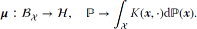
Assuming that K(x, ⋅) is bounded for any ![]() , we can show that for any ℙ, letting
, we can show that for any ℙ, letting ![]() , the
, the ![]() , for all
, for all ![]() .
.
The primal optimization problem for the OC‐SMM can be formulated in an analogous way to the OC‐SVM (or ν‐SVM):

constrained to
where the meaning of the hyperparameters stands the same, but they are now instead associated with distributions (note the appearance of the mean distribution appears as a constraint in Equation 11.60). By operating in the same way, one obtains that the dual form is again a QP problem that depends on the inner product ![]() that can be computed using the mean map kernel function:
that can be computed using the mean map kernel function:
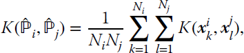
where ![]() are the samples belonging to distribution i, and Ni represents its cardinality. Links to MATLAB source code for this method are available on the book’s web page.
are the samples belonging to distribution i, and Ni represents its cardinality. Links to MATLAB source code for this method are available on the book’s web page.
11.7 Tutorials and Application Examples
We next include a set of simple examples for providing insight on the topics of this chapter. Some of the functions are not included in the text, as indicated, but the interested reader can obtain the code from the book’s repository.
11.7.1 Example on Kernelization of the Metric
Let us see the relation described in this chapter for kernelization of the metric in a simple code example, given in Listing 11.3. We generate the well‐known Swiss roll dataset, then compute both the Euclidean distances in the original space and the Hilbert space (with a specific σ parameter for the kernel).
Figure 11.4 illustrates the behavior of the distance values in the input space against the distances computed in the Hilbert space. We can see how some of the distances have decreased values with respect to the input space in the range [0, 1/2] and the remaining distances have increased in the Hilbert space. The shape of the curve shows the nonlinear relation between distances.

Figure 11.4 Distance values computed in input space against computed in the Hilbert space (through reproducing kernels). This figure is generated with Listing 11.3.
11.7.2 Example on Kernel k‐Means
The code in Listing 11.4 runs the k‐means function of MATLAB and an implementation of kernel k‐means for the problem of concentric rings. Figure 11.5 illustrates the final solution of both methods: k‐means could not achieve a good solution (left) compared to kernel k‐means which finally converges to the correct solution (right).

Figure 11.5 Results obtained by k‐means (left) and kernel k‐means (right) in the concentric ring problem.
11.7.3 Domain Description Examples
This section compares different standard one‐class classifiers and kernel detectors: Gaussian (GDD), mixture of Gaussians (MoGDD), k‐NN (KnnDD), and the SVDD (with the RBF kernel). All one‐class domain description classifiers have a parameter to adjust, which is the fraction rejection, that controls the percentage of target samples the classifier can reject during training. Some other parameters need to be tuned depending on the classifier. For instance, the Gaussian classifier has a regularization parameter in the range [0, 1] to estimate the covariance matrix, using all training samples or only diagonal elements.
With regard to the mixture of Gaussian classifier, four parameters must be adjusted: the shape of the clusters to estimate the covariance matrix (e.g., full, diagonal, or spherical), a regularization parameter in the range [0, 1] used in the estimation of the covariance matrices, the number of clusters used to model the target class, and the number of clusters to model the outlier class. The most important advantage of this classifier with respect to the Gaussian classifier, apart from the obvious improvement of modeling a class with several Gaussian distributions, is the possibility of using outliers information when training the classifier. This allows the tracing of a more precise boundary around the target class, improving classification results notably. However, having a total of five parameters to adjust constitutes a serious drawback for this method, making it difficult to obtain a good working model.
With respect to the k‐NN classifier, only the number of k neighbors used to compute the distance of each new sample to its class must be tuned. Finally, for the SVDD, the width of the RBF kernel (σ) has to be adjusted. In all the experiments, except the last one, σ is selected among the following set of discrete values between 5 and 500. It is worth stressing here that the SVDD is one of the methods among those considered, together with the mixture of Gaussians, that allows one to use outliers information to better define the target class boundary. In addition, it has the important advantage that only two free parameters have to be adjusted, thus making it relatively easier to define a good model.
In all the experiments, 30% of the samples available are used to train each classifier. In order to adjust free parameters, a cross‐validation strategy with four folds is employed. Once the classifier is trained and adjusted, the final test is done using the remaining 70% of the samples. In all our experiments, we used the dd_tools and the libSVM software packages.
Two different synthetic problems are tested here. In each problem, binary classification is addressed, thus having two sets of targets and outliers. Each class contains 500 samples generated from different distributions. The two problems analyzed are mixture of two Gaussian distributions and a mixture of Gaussian and logarithmic distributions; both of them are strongly overlapped. Our goal here is testing the effectiveness of the different methods with standard and simple models but in very critical conditions on the overlapping of class distributions.
In order to measure the capability of each classifier to accept targets and reject outliers, the confusion matrix for each problem is obtained, and the kappa coefficient (κ) is estimated, which gives a good trade‐off between the capability of the classifier to accept its samples (targets) and reject the others (outliers). Table 11.2 shows the results for the tests, and Figure 11.6 shows graphical representations of the classification boundary defined by each method. In each plot, the classifier decision boundary levels is represented with a blue curve. Listing 11.5 shows the code that has been used for generating these results. Functions getsets.m, train_basic.m, and predict_basic.m can be seen in the code (not included here for brevity).
Table 11.2 The coefficient of accuracy κ and the overall accuracy in parentheses (percent) obtained for the synthetic problems.
| GDD | MoGDD | KnnDD | SVDD | |
| Two Gaussians | 0.52 (76.0) | 0.67 (83.5) | 0.56 (78.1) | 0.63 (81.7) |
| Mixed Gaussian–log | 0.65 (82.7) | 0.77 (88.8) | 0.48 (74.1) | 0.78 (89.4) |

Figure 11.6 Plot of the decision boundaries obtained with GDD, MoGDD, KnnDD, and SVDD for the two Gaussians problem (top) and the mixed Gaussian–logarithm problem (bottom). Note the semilogarithmic scale in this latter case.
Several conclusions can be obtained from these tests. First, MoGDD and SVDD obtain the highest accuracies in our problems. When mixing two Gaussians, none of the classifiers shows a good behavior, as in our synthetic data the distributions are strongly overlapped. This is a common situation in the remote‐sensing field when trying to classify classes very similar to each other. Mixture of overlapped Gaussian and logarithmic features is a difficult problem. In this synthetic example, we can see that the SVDD performs slightly better, since it does not assume any a priori data distribution.
11.7.4 Kernel Spectral Angle Mapper and Kernel Orthogonal Subspace Projection Examples
The following two experiments have the aim of comparing KSAM and KSOM (and also their linear versions) in terms of real data problems. In the former, a QuickBird image of a residential neighborhood of Zürich, Switzerland, is used for illustration purposes. The image size is (329 × 347) pixels. A total of 40 762 pixels were labeled by photointerpretation and assigned to nine land‐use classes (see Figure 11.8). Four target detectors are compared in the task of detecting the class “Soil”: OSP (Harsanyi and Chang, 1994), its kernel counterpart KOSP (Kwon and Nasrabadi, 2007), standard SAM (Kruse et al., 1993), and the extension KSAM.
Figure 11.7 shows the receiver operating characteristic (ROC) curves and the area under the ROC curves (AUC) as a function of the kernel length‐scale parameter σ. KSAM shows excellent detection rates, especially remarkable in the inset plot (note the logarithmic scale). Perhaps more importantly, the KSAM method is relatively insensitive to the selection of the kernel parameter compared with the KOSP detector, provided that a large enough value is specified.

Figure 11.7 (a) ROC curves and (b) AUC as a function of the kernel length‐scale parameter.
The latter experiments allow us to use a traditional prescription to fix the RBF kernel parameter σ for both KOSP and KSAM as the mean distance among all spectra, dM. Note that after data standardization and proper scaling, this is a reasonable heuristic σ ≈ dM = 1. The thresholds were optimized for all methods. OSP returns a decision function strongly contaminated by noise, while the KOSP detector results in a correct detection. Figure 11.8 shows the detection maps and the metric learned. The (linear) SAM gives rise to very good detection but with strong false alarms in the bottom left side of the image, where the roof of the commercial center saturates the sensor and thus returns a flat spectrum for its pixels in the morphological features. As a consequence, both the target and the roof vectors have flat spectra and their spectral angle is almost null. KSAM can efficiently cope with these (nonlinear) saturation problems. In addition, the metric space derived from the kernel suggests high discriminative (and spatially localized) capabilities.

Figure 11.8 Detection results for different algorithms (accuracy, κ statistic).
11.7.5 Example of Kernel Anomaly Change Detection Algorithms
In this section we show the usage of the proposed methods in several simulated and real examples of pervasive and anomalous changes. Special attention is given to detection ROC curves, robustness to number of training samples, low‐rank approximation of the solution, and the estimation of Gaussianity in kernel feature space. Comparisons between the hyperbolic (HACD), elliptical (EC), kernelized (K‐HACD), and elliptical kernelized (K‐EC‐HACD) versions of the algorithms are included. Results can be reproduced using the script demoKACD.m available in the book’s repository.
This example follows the simulation framework used in Theiler (2008). The dataset (see Figure 11.9) is an image acquired over the Kennedy Space Center, Florida, on March 23, 1996, by the Airbone Visible Infrared Imaging Spectrometer (AVIRIS). The data were acquired from an altitude of 20 km and have a spatial resolution of 18 m. After removing low SNR and water absorption bands, a total of 176 bands remain for analysis. More information can be found at http://www.csr.utexas.edu/. To simulate a pervasive change, global Gaussian noise, ![]() , was added to all the pixels in the image to produce a second image. Then, anomalous changes are produced by scrambling the pixels in the target image. This yields anomalous change pixels whose components are not individually anomalous.
, was added to all the pixels in the image to produce a second image. Then, anomalous changes are produced by scrambling the pixels in the target image. This yields anomalous change pixels whose components are not individually anomalous.

Figure 11.9 Hyperspectral image (left panel) captured with AVIRIS, and four illustrative chips of simulated changes (right panel). The original (leftmost) image is used to simulate an anomalous change image (rightmost) by adding Gaussian noise and randomly scrambling 1% of the pixels.
In all experiments, we used hyperbolic detectors (i.e., βx = βy = 1), as they generalize RX and chronocrome ACD algorithms, and have shown improved performance (Theiler et al., 2010). In this example, we use the SAM kernel, which is more appropriate to capture hyperspectral pixel similarities than the standard RBF kernel. We tuned all the parameters involved (estimated covariance Cz and kernel Kz, ν for the EC methods, length‐scale σ parameter for the kernel versions) through standard cross‐validation in the training set, and show results on the independent test set. We used λ = 10−5/N, where N is the number of training samples, and the σ kernel length‐scale parameter is tuned in the range of 0.05–0.95 percentiles of the distances between all training samples, dij.
Figure 11.10 shows the ROC curves obtained for the linear ACD and KACD methods. The dataset was split into small training sets of only 100 and 500 pixels, and results are given for 3000 test samples. The results show that the kernel versions improve upon their linear counterparts (between 13–26% in Gaussian and 1–5% in EC detectors). The EC variants outperform their Gaussian counterparts, especially in the low‐sized training sets (+30% over HACD and +18% over EC‐HACD in AUC terms). Also noticeable is that results improve for all methods when using 500 training samples. The EC‐HACD is very competitive compared with the kernel versions in terms of AUC, but still K‐EC‐HACD leads to longer tails of false‐positive detection rates (right figure, inset plot in log‐scale).

Figure 11.10 ROC curves and AUC obtained for the hyperspectral experiments by linear and kernel detectors for 100 (up) and 500 (down) training examples.
11.7.6 Example on Distribution Embeddings and Maximum Mean Discrepancy
Let us exemplify the use of the concept of distribution embeddings and MMD in a simple example comparing two distributions ℙx and ℙy. We draw samples from (i) two Gaussians with different means, (ii) Gaussians with the same means but different variance, and (iii) from a Gaussian and a Laplace distributions. A code snippet is given in Listing 11.6 illustrating the ability of MMD to detect such differences. The results obtained are shown in Figure 11.11.
Figure 11.11 The two‐sample problem reduces to detecting whether two distributions ℙx and ℙy are different or not. Up, left: whenever we have two Gaussians with different means one can assess statistical differences by means of a standard t test of different means (the distance between the empirical means is dxy := ∥μx − μy∥ = 3.91). Up, right: when we have two Gaussians with the same means but different variance (dxy = 0.02), the idea may be to look (down, left) at difference in means of transformed random variables (for the Gaussian case, second‐order features of the form x2 suffice for discrimination, dxy = 13.26). Down, right: when distributions come from different pdfs (in this case, Gaussian and Laplace distributions) with the same mean and variance, one has to map the RVs to higher order features for discrimination (dxy = 0.06 in the original domain and dxy = 75.80 for a fifth‐order mapping).
11.8 Concluding Remarks
This chapter treated the relevant topic of clustering and anomaly detection with kernels. The field is undoubtedly in the core of machine learning, and has many practical implications. The conceptual/philosophical problem of defining regularity, cluster, membership, and anomaly is an elusive one, so that there are the proper statistical definition of significant difference, hypothesis testing, and similarity measures between probabilities. Consequently, many methods and approaches have been proposed to tackle these problems. We reviewed several families available and related to a certain extent. We organized the kernel‐based approaches systematically, and revised them organized in a simple taxonomy: (1) clustering, (2) density estimation (sometimes referred as to domain description), (3) matched subspace detectors, (4) anomaly change detection, and (5) statistical hypothesis testing.
The treatment in this chapter was far from exhaustive; rather, we tried to cover the main fields and to give an intuition on the relations among particular approaches. We observed clear links between clustering, subspace projection, and density estimation methods. The first essentially considered density characterization via kernelization of the metric or the algorithm, and the last relied on sound concepts of distribution embeddings.
We should also mention that the field of clustering and anomaly detection has arrived at a certain point of maturity with the introduction of relevant new paradigms from machine learning, such as SSL and AL, and from signal processing such as online and adaptive filtering. In many problems, introducing some labeled information properly helps in discerning the anomaly; also, including the user in the loop via active detection may help the detectors. The problem of anomaly detection in signal processing problems has to do very often with adaptation to changing environments/channels, so both adapting the classifier and/or the data representation has also been approached in the field. Other relevant issues to the DSP community, such as change‐point detection, were intentionally omitted for the sake of conciseness.
The number of applications of the techniques presented will probably increase in the following years. The identification of events that are far from normal is an extremely appealing target for many real science and engineering applications, from health to traffic monitoring and climate science. In this setting, many big data environments or long‐term monitoring from diverse kinds and nature will require DSP techniques running in parallel or even embedded with solid anomaly detection and domain description algorithms.
11.9 Questions and Problems
- Exercise 11.9.1 Given an arbitrary dataset, obtain and compare the clustering solutions for k = {2, 3, 4, 5} using k‐means and kernel k‐means with (a) the linear kernel and (b) the RBF Gaussian kernel for several values of the length‐scale σ parameter.
- Exercise 11.9.2 Obtain Equations 11.17 and 11.18.
- Exercise 11.9.3 Demonstrate these latter two equations in Equation 11.20.
- Exercise 11.9.4 Obtain the update rule for αjl in Equation 11.33.
- Exercise 11.9.5 Demonstrate that SVDD and OC‐SVM reduce to the same equations when using the RBF kernel.
- Exercise 11.9.6 Exploit the kernelization of the metric in the SAM similarity measure, which is commonly used in change detection, and that is given by(11.62)
where 0 ≤ θ ≤ π/2. Show that KSAM is a valid Mercer kernel and that KSAM is universal.
- Exercise 11.9.7 A critical issue in kernel dependence estimation is about the selection of the kernel function and its hyperparameters. Very often one simply selects the SE kernel and sets the σ length‐scale to the average distance between all samples. Test other ways based on the field of density estimation (e.g., Silverman’s rule and related heuristics)). Figure out a way to tune Hilbert–Schmidt independence criterion (HSIC) parameters in a supervised manner.
- Exercise 11.9.8 Derive the HSIC empirical estimate with regard to the σ parameter for the sake of optimization.
- Exercise 11.9.9 Demonstrate the ECd kernel versions in Equations 11.55 and 11.56.
- Exercise 11.9.10 The performance of the linear and kernel EC algorithms can be severely affected by the value of ν. Theiler et al. (2010) suggested a heuristic based on the ratio of moments of the distribution, ν = 2 + mκm/(κm − (d + m)), where κm = 〈rm+2〉/〈rm〉,
 and fixed m = 1 to control the impact of outliers. Discuss on the motivation, and its suitability in the kernel case. Can you say anything about the Gaussianity in feature spaces?