Chapter Nine MPEG 1 Audio Compression
The compact disc (CD) made digital audio a consumer product almost overnight. In a matter of two decades, it became difficult to even find a 33-rpm vinyl phonograph record. Consumers no longer had to put up with the annoying aspects of analog media such as flutter, wow, hiss, and other artifacts. Instead, they could have approximately an hour of flawless audio play on a small, compact, robust medium, with a player costing under $200.
To achieve its audio quality, the CD contains samples of an analog signal at 44.1 Ksamples per second and 16 bits per sample, or 705.6 Kbps. Because two analog signals are needed to create stereo, the 705.6 Kbps is multiplied by two, or 1,411.2 Kbps. If this is compared to the required services per transponder given in Chapter 8, it is clear that, if CD-quality audio is desired, the audio would take up too large a fraction of the total bit rate if not compressed by a significant amount.
The Compression Problem: DBS audio has 24-millisecond input frames, and samples each of the analog inputs at 48 Ksamples per second and 16 bits per sample. The output is 192 Kbps for both audio outputs combined.
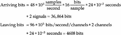
Therefore, audio compression must reduce the number of bits by 36,864 / 4608 = 8; in other words, a compression ratio of 8:1. MPEG Audio provides this compression.
It should be noted that while the MPEG Audio standard was developed as part of an integrated audio/video standard, the audio part can be used alone. In fact, one of the more surprising results of DBS service has been the popularity of the audio service. DIRECTV⁜ provides 28 ‘commercial-free’ audio channels with the menu indicating the music type. At our house we frequently leave the music on during the day, just for background.
9.1 MPEG Audio Compression Overview
MPEG 1 Audio (ISO 11172-3) is oriented toward high-quality stereo audio. At the present time, all known DBS systems use Layer II of MPEG 1 Audio, at 192 Kbps, for stereo delivery.
MPEG 1 Audio provides a very large number of options in both sampling frequency, output bit rate, and three ‘layers.’ The MPEG 1 Audio Layers are not layers in the sense that one builds on the other. Rather, they are layers in the sense that a higher-numbered layer decoder can decode a lower-numbered layer. In this book, the discussion is limited to the particular options used in DBS systems.
ISO 11172-3 defines only a decoder. However, including an encoder description makes it easier to understand.
9.1.1 Encoding
Prior to MPEG 1 Audio, audio compression usually consisted of removing statistical redundancies from an electronic analog of the acoustic waveforms. MPEG 1 Audio achieved further compression by also eliminating audio irrelevancies by using psychoacoustic phenomena such as spectral and temporal masking. One way to explain this is that if the signal at a particular frequency is sufficiently strong, weaker signals that are close to this frequency cannot be heard by the human auditory system and, therefore, can be neglected entirely.
In general, the MPEG 1 Audio encoder operates as follows. Input audio samples are fed into the encoder. For DBS, these samples are at a sample rate of 48 Ksamples per second (for each of the stereo pairs), so this rate will be used exclusively in the rest of this chapter. Each sample has 16 bits of dynamic range. A mapping creates a filtered and subsampled representation of the input audio stream. In Layer II, these 32 mapped samples for each channel are called subband samples.
In parallel, a Psychoacoustic Model performs calculations that control quantizing and coding. Estimates of the masking threshold are used to perform this quantizer control. The bit allocation of the subbands is calculated on the basis of the signal-to-mask ratios of all the subbands. The maximum signal level and the minimum masking threshold are derived from a Fast Fourier Transform (FFT) of the sampled input signal.
Of the mono and stereo modes possible in the MPEG 1 Audio standard, Joint Stereo (left and right signals of a stereo pair coded within one bitstream with stereo irrelevancy and redundancy exploited) is used in Layer II—hence, DBS. Within Joint Stereo, the intensity stereo option is used. All DBS systems use 192 Kbps for this stereo pair.
9.1.2 Decoding
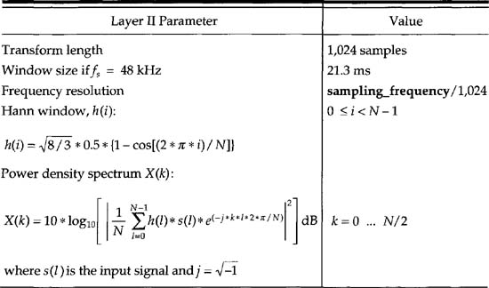
The basic structure of the audio decoder reverses the encoding process. Bit-stream data is fed into the decoder. First, the bitstream is unpacked with the main data stream separated from the ancillary data. A decoding function does error detection if an error_check has been applied in the encoder. The bitstream data is then unpacked to recover the various pieces of information. A reconstruction function reconstructs the quantized version of the set of mapped samples. The inverse mapping transforms these mapped samples back into a Pulse Code Modulation (PCM) sequence. The output presentation is at 48 Ksamples per second for each of the two stereo outputs. The specific parameters utilized by DBS are shown in Table 9.1.
Table 9.1 DBS Audio Parameters

9.2 Description of the Coded Audio Bitstream
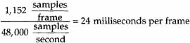
The basic building block of the MPEG 1 Audio standard is an Audio Frame. An Audio Frame represents a duration equal to the number of samples divided by the sample rate. For DBS, Layer II has 1,152 samples at a sample rate of 48 Ksamples per second. The frame period is then
Audio frames are concatenated to form audio sequences.
Audio Frame: An audio frame is a fixed-length packet in a packetized bitstream. In Layer II, it consists of 1,152 samples each of stereo audio input plus the rest of the bits comprising the packet. Each packet has a total of 4,608 bits. It starts with a syncword, and ends with the byte before the next syncword.
Each audio frame consists of four separate parts:
1. All packets in a packetized bitstream contain a header that provides synchronization and other information required for a decoder to decode the packet.
2. The error_check (optional) contains 16 bits that can detect errors in storage or transmission.
3. The audio_data is the payload of each packet. It contains the coded audio samples and the information necessary to decode them.
4. The ancillary_data has bits that may be added by the user.
Each of these is described in the following sections.
9.2.1 Header
![]()
The first 32 bits (4 bytes) of an Audio Frame are header information.
The syncword is the 12-bit string 0xFFF.
The ID is a 1-bit flag that indicates the identification of the algorithm; it is ‘1’ for all DBS systems.
The layer parameter is the 2 bits, ‘10’, that indicates Layer II.
The protection_bit is a 1-bit flag that indicates whether error detection bits have been added to the audio bitstream. It is a ‘1’ if no redundancy has been added, ‘0’ if redundancy has been added.
The bitrate_index is a 4-bit parameter that indicates the bit rate. In the case of DBS, the value is ‘1010’ to indicate 192 Kbps for the stereo.
The sampling_frequency is a 2-bit parameter that indicates sampling frequency. For DBS, the value is ‘01’, indicating 48 Ksamples per second.
The padding_bit is not required at 48 Ksamples per second.
The private_bit is for Private use.
The mode is a 2-bit parameter that indicates the channel mode. For DBS, the value is ‘01’, indicating joint stereo. In Layer II, joint stereo is intensity stereo.
Figure 9.1 shows the operation of intensity stereo. For subbands less than sb_bound (bound), there are separate left and right audio bitstreams. For subbands of sb_bound and larger, a single bitstream that is the sum of the left and right values is transmitted. The left and right signal amplitude can be controlled by a different scalefactor.
Figure 9.1 Intensity Stereo

bound and sblimit are parameters used in intensity_stereo mode. In intensity_stereo mode bound is determined by mode_extension.
The mode_extension is a 2-bit parameter that indicates which subbands are in intensity_stereo. All other subbands are coded in stereo. If the mode_extension is considered as a decimal number dec, the subbands dec * 4 + 4 to 31 are coded in intensity stereo. For example, if mode_extension is ‘11’, dec = 3 and dec * 4 + 4 = 16. Thus, subbands 16 through 31 are coded in intensity_stereo.
The copyright flag is 1 bit. A ‘1’ means the compressed material is copyright protected.
The original/copy is ‘0’ if the bitstream is a copy, ‘1’ if it is an original.
The emphasis is a 2-bit parameter that indicates the type of deemphasis that is used. For DBS, the parameter is ‘01’, indicating 50/15-microsecond deemphasis.
9.2.2 error_check
The error_check is an optional part of the bitstream that contains the Cyclical Redundancy Check (crc_check), a 16-bit parity-check word. It provides for error detection within the encoded bitstream (see Appendix E).
9.2.3 audio_data, Layer II
The audio_data is the payload part of the bitstream. It contains the coded audio samples, and information on how these audio samples are to be decoded. The following are the key elements of audio_data, Layer II.
allocation[ch][sb]—[ch] indicates the left or right stereo channel, ‘0’ for left and ‘1’ for right, [sb] indicates the subband. allocation[ch][sb] is a 4-bit unsigned integer that serves as the index for the algorithm to calculate the number of possible quantizations (see Possible Quantization per Subband section later in this chapter).
scfsi[ch][sb]—This provides scalefactor selection information on the number of scalefactors used for subband[sb] in channel[ch]. In general, each of the three 12 subband samples requires a separate scalefactor. In this case, scfsc[sb] = ‘00’. If all three of the parts can be represented by a single scalefactor, scfsi[sb] = ‘10’. If two scalefactors are required, scfsi[sb] = ‘01’ if the first scalefactor is valid for parts 0 and 1 and the second for part 2; scfsi[sb] = ‘11’ if the first scalefactor is valid for part 0 and the second for parts 1 and 2.
scalefactor[ch][sb][p]—[p] indicates one of the three groupings of sub-band samples within a subband. scalefactor[ch][sb][p] is a 6-bit unsigned integer which is the index to the scalefactor calculation in the Possible Quantization per Subband section later in this chapter.
grouping[ch][sb]—This is a 1-bit flag that indicates if three consecutive samples use one common codeword and not three separate codewords. It is true if the calculation in the Possible Quantization per Subband section creates a value of 3, 5, or 9; otherwise it is false. For subbands in intensity_stereo mode, the grouping is valid for both channels. samplecode[ch][sb][gr]—[gr] is a granule that represents 3 * 32 subband samples in Layer II. samplecode[ch][sb][gr] is the code for three consecutive samples of [ch], [sb], and [gr].
sample[ch][sb][n]—This is the coded representation of the nth sample in [sb] of [ch]. For the subbands here, sb_bound, and hence in intensity_ stereo mode, this is valid for both channels.
9.2.4 ancillary_data
This MPEG 1 Audio bitstream has provisions for user supplied data. The number of ancillary bits (no_of_ancillary_bits) used must be subtracted from the total bits per frame. Since the frame length is fixed, this subtracts from the bits available for coding the audio samples and could impact audio quality.
9.3 Detailed Encoder
The MPEG 1 Audio algorithm is what is called a psychoacoustic algorithm. The following sections describe the four primary parts of the encoder.
9.3.1 The Filterbanks
The Filterbanks provide a sampling of the frequency spectrum for each of the 32 input samples. These Filterbanks are critically sampled, which means there are as many samples in the analyzed (frequency) domain as there are in the time domain. For the encoder, the Filterbank is called the ‘Analysis Filter-bank’ (see details in next section); in the decoder, the reconstruction filters are called the ‘Synthesis Filterbank’ (see details at end of this chapter).
In Layer II, a Filterbank with 32 subbands is used. In each subband, there are 36 samples that are grouped into three groups of 12 samples each.
Input High-Pass Filter
The encoding algorithms provide a frequency response down to D.C. It is recommended that a high-pass filter be included at the input of the encoder with a cut-off frequency in the range of 2 Hz to 10 Hz. The application of such a filter avoids wasting precious coding bits on sounds that cannot be heard by the human auditory system.
Analysis Subband Filterbank
![]()
An analysis subband Filterbank is used to split the broadband signal with sampling frequency fs into 32 equally spaced subbands with sampling frequencies fs/32. The algorithm for this process with the appropriate formulas is given in the following algorithm description.
Analysis Filterbank Algorithm
1. Shift 32 new audio samples into a shift register.

2. Window by multiplying each of the X values by an appropriate coefficient.
![]()
3. Next form a 64-component vector Y, as follows:

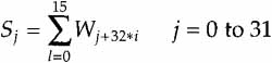
4. Create subband outputs:
![]()
Figure 9.2 shows the values Di that are used in the Synthesis Subband Filter. The Ci values used in Equation (9.1) are obtained by dividing the D values by 32 for each index. Tables in the standard represent both the C and D values. I find the curves (see figure) more compact and instructive.
Figure 9.2 Parameter D Coefficients

9.3.2 Psychoacoustic Model
![]()
Psychoacoustic Model 1 is used with all known DBS systems and will be the only Psychoacoustic Model discussed. For Psychoacoustic Model 1, the FFT has a 1,024 sample window (see Analysis that follows). While this is less than the number of samples in a frame, it does not cause serious impact on quality.
The end result of the Psychoacoustic Model is the following signal-to-mask ratio:
![]()
which must be computed for every subband n. Lsb(n) is the sound pressure level (SPL) in each subband n. LTmin(n) is the minimum masking level in each subband n. In the following sections, we show how each of these is computed.
FFT Analysis: The masking threshold is derived from the FFT output. A form of raised cosine filter, called a Harm window, filters the input PCM signal prior to calculating the FFT. The windowed samples and the Analysis Filterbank Outputs have to be properly aligned in time. A normalization to the reference level of 96 dB SPL has to be done in such a way that the maximum value corresponds to 96 dB.
Sound Pressure Level Calculation
Equation (9.5) requires calculation of the SPL Lsb(n) in subband n. Lsb(n) is determined from
![]()
X(k) in subband n, where X(k) is the sound pressure level with index k of the FFT with the maximum amplitude in the frequency range corresponding to subband n. The expression scfmax(n) is the maximum of the three scalefactors of subband n within an Audio Frame. The ‘-10 dB’ term corrects for the difference between peak and RMS level. The SPL Lsb(n) is computed for every subband n.
The second step in calculating Equation (9.5) is to calculate LTmin(n), which turns out to be a rather involved process. The minimum masking level, LTmin(n), in subband n is determined by the following expression:
![]()
which requires calculation of LTg(i), the global masking threshold at the ith frequency sample.

Thus, LTg(i) requires the calculation of LTq(i), the Absolute Threshold, LTtm[z(j), z(i)], the individual Masking Threshold for tonal maskers, and LTnm[z(j), z(i)], the Individual Masking Threshold for nontonal maskers.
Determining the Absolute Threshold
When a tone of a certain amplitude and frequency is present, other tones or noise near this frequency cannot be heard by the human ear. The maximum level of the lower amplitude signal that is imperceptible is called the Masking Threshold. There is a threshold, which is a function of frequency, below which a tone or noise is inaudible regardless of whether there is a masker or not. This threshold is called the Absolute Threshold and is shown if Figure 9.3.
Figure 9.3 Absolute Threshold
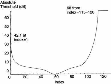
The Absolute Threshold is labeled LTq(k) and is also called threshold in quiet. In the ISO Standard, Table D.lf gives a set of index numbers, Frequencies for Critical Bands, Critical Band Rates (CBRs), and the Absolute Threshold. The index runs from 1 to 126. For most work, the values of these parameters can be determined from the curves in Figures 9.3,9.4, and 9.5.
Figure 9.4 Critical Frequency Band
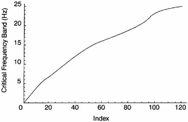
Figure 9.5 Critical Frequency

Individual Masking Threshold Determination
Tonal maskers are close to sinusoids and have spectra that are near impulses. On the other hand, nontonal maskers exhibit noiselike characteristics. The individual masking thresholds of both tonal and nontonal components are given by the following expressions:
![]()
![]()
In Equations (9.9) and (9.10), LTtm and LTnm are the individual Masking Thresholds at CBR z in Bark of the masking component at the Critical Band Rate of the masker zm in Bark. The values in dB can be either positive or negative. Equations (9.9) and (9.10) require the calculation of five new parameters: Xnm[z(j)], Xtm[z(j)], a νnm[z(j)], a νtm[z(j)], and νf[z(j), z(i)].
Finding of Xnm[z(j)] and Xtm[z(j)]
It is necessary to discriminate between them when calculating the Global Masking Threshold from the FFT spectrum. This step starts with the determination of local maxima, then extracts tonal components and calculates the intensity of the nontonal components within a bandwidth of a critical band. The following describes how boundaries of the critical bands can be determined.
The ISO Standard, in Table D.2f, gives these values, which are just a subset of 27 of the 126 values from Table D.lf. The index runs from 0 to 26, representing the indices 1, 2, 3, 5, 7, 9, 12, 14, 17, 20, 24, 27, 32, 37, 42, 49, 53, 59, 65, 73, 77, 82, 89, 97, 103, 113, and 126. The values for the frequency and band can be determined from Figures 9.4 and 9.5.
The bandwidth of the critical bands varies with the center frequency, with a bandwidth of about only 0.1 kHz at low frequencies and with a bandwidth of about 4 kHz at high frequencies. It is known from psychoacoustic experiments that the ear has a better frequency resolution in the lower than in the higher frequency region. To determine if a local maximum may be a tonal component, a frequency range, df, around the local maximum is examined. For frequencies up to 3 kHz, df = 93.75 Hz. For frequencies from 3 kHz to 6 kHz, df = 140.63 Hz. For frequencies from 6 kHz to 12 kHz, df = 281.25 Hz, and for frequencies between 12 kHz and 24 kHz, df = 562.5 Hz.
To make lists of the spectral lines X(k) that are tonal or nontonal, the following five operations are performed:
1. Selection of local maxima candidates—A spectral line X(k) is labeled as a local maximum if
![]()
2. Selection of tonal components—A local maximum is put in the list of tonal components if
![]()
where j is chosen according to the subband index range. For the index between 2 and 63, j = ±2; for the index greater than or equal to 63 and less than 127, j = ±2, ±3; for index greater than or equal to 127 and less than 255, j = ±2, ±3, ±4, ±5, and ±6. This step checks how wide the spectrum of the local maximum candidates is.
3. Sound pressure level—The SPL is calculated next. For each k, where X(k) has been found to be a tonal component,
![]()
Next, all spectral lines within the examined frequency range are set to ![]() dB.
dB.
4. Nontonal components—The nontonal (noise) components are calculated from the remaining spectral lines. To calculate the nontonal components from spectral lines X(k), the critical bands z(k) are determined using Figure 9.5. In Layer II, 26 critical bands are used for the 48 kHz sampling rate.
5. Calculation of the power—Within each critical band, the power of the spectral lines (remaining after the tonal components have been zeroed) are summed to form the SPL of the new nontonal component, Xnm(k), corresponding to that critical band.
Decimation of Tonal and Nontonal Masking Components
Decimation is a procedure that is used to reduce the number of maskers that are considered for the calculation of the Global Masking Threshold. In the discussion here, a Bark is the critical band unit.
Xtm(k) or Xnm(k) are considered for the calculation of the Masking Threshold only if they are greater than LTq(k) for each index k.
Decimation of two or more tonal components within a distance of less than 0.5 Bark: Keep the Xtm[z(j)] with the highest power, and remove the smaller component(s) from the list of tonal components. For this operation, a sliding window in the critical band domain is used with a width of 0.5 Bark.
The term aν is called the masking index and is different for tonal and nontonal maskers (a’tm and a’nm). The masking indices aνtm and aνnm are empirically determined. For tonal maskers it is given by
![]()
and for nontonal maskers by
![]()
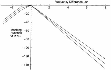
The term vf is called the masking function of the masking component Xtm[z(j)] and is characterized by different lower and upper slopes, which depend on the distance in Bark, dz = z(i) – z(j), to the masker. In this expression, i is the index of the spectral line at which the masking function is calculated and; is that of the masker. CBRs z(j) and z(i) can be found in Figure 9.4.
The masking function is defined in terms of dz and X[z(j)]. It is a piece-wise linear function of dz, nonzero for -3 ≤ dz < 8 Bark. The parameter νf depends only weakly on X[z(j)]. This can be seen in Figure 9.6. LTtm and LTnm are set to ![]() dB if dz < -3 Bark, or dz >= 8 Bark.
dB if dz < -3 Bark, or dz >= 8 Bark.
Figure 9.6 Masking Function for X(z(j)) = -10,0,10
9.3.3 Bit Allocation
The process of allocating bits to the coded parameters must attempt to simultaneously meet both the bit rate requirements and the masking requirements. If insufficient bits are available, it must use the bits at its disposal in order to be as psychoacoustically inoffensive as possible. In Layer II, this method is a bit allocation process (i.e., a number of bits are assigned to each sample, or group of samples, in each subband).
Scalefactor Calculation
The scalefactors can be stored in a table (see Table B.1 in the ISO Standard) or calculated. Using the number 1.2599210498949, the scalefactor value for each index n is
![]()
where n ranges from 0 to 62. For each subband, a scalefactor is calculated for every 12 subband samples. The maximum of the absolute value of these 12 samples is determined. The lowest value calculated from Equation (9.16) that is larger than this maximum is used as the scalefactor.
Coding of Scalefactors
Call the index determined from the algorithm of the Possible Quantization per Subband section scf. Because there are three of these per subband, they are labeled scf1, scf2, and scf3. First, the two differences, dscf1 and dscf2, of the successive scalefactor indices—scf1, scf2, and scf3—are calculated:
![]()
The class of each of the differences is determined as follows:
• If dscf is less than or equal to -3, the class is 1.
• If dscf is between -3 and 0, the class is 2.
• If dscf equals 0, the class is 3.
• If dscf is greater than 0 but less than 3, the class is 4.
• If dscf is greater than 3, the class is 5.
Because there are two dscf, there are two sets of classes.
The pair of classes of differences indicates the entry point in the following algorithm to get the calculations in ISO Table C.4, ‘Layer II Scalefactor Transmission Patterns.’ Because there are two sets of five classes, there are 25 possibilities:
• For the class pairs (1,1), (1,5), (4,5), (5,1), and (5,5),1 all three scalefactors are used, the transmission pattern is 123, and the Selection Information is ‘00’.
1 “1,” “2,” and “3” mean the first, second, and third scalefactor within a frame, and “4” means the maximum of the three scalefactors. The information describing the number and the position of the scalefactors in each subband is called ‘Scalefactor Selection Information.’
• For the class pairs (1,2), (1,3), (5,2), and (5,3), the scalefactors used are 122, the transmission pattern is 12, and the Selection Information is ‘11’.
• For the class pairs (1,4) and (5,4), the scalefactors are 133, the transmission pattern is 13, and the Selection Information is ‘11’.
• For the class pairs (2,1), (2,5), and (3,5), the scalefactors used are 113, the transmission pattern is 13, and the Selection Information is ‘01’.
• For classes (2,2), (2,3), (3,1), (3,2), and (3,3), the scalefactors are 111, the transmission pattern is 1, and the Selection Information is ‘01’.
• For class pairs (3,4) and (4,4), the scalefactors are 333, the transmission pattern is 3, and the Selection Information is ‘01’.
• If the class pairs are (4,1), (4,2), and (4,3), the scalefactors are 222, and the Selection Information is ‘01’.
• Finally, class pair (2,4) uses the scalefactors 444, the transmission pattern 4, and Selection Information ‘01’.
Scalefactor Selection Information Coding
For the subbands that will get a nonzero bit allocation, the Scalefactor Selection Information (scfsi) is coded by a 2-bit word. This was noted previously for Layer II Scalefactor Transmission Patterns.
Bit Allocation
Before starting the bit allocation process, the number of bits, “adb”, that are available for coding the payload must be determined. This number can be obtained by subtracting from the total number of available bits, “cb”; the number of bits needed for the header, “bhdr” (32 bits); the CRC checkword, “bcrc” (if used) (16 bits); the bit allocation, “bbal”; and the number of bits, ‘banc,’ required for ancillary data:
![]()
Thus, adb bits are available to code the payload subband samples and scale-factors. The allocation approach is to minimize the total noise-to-mask ratio over the frame.
Possible Quantization per Subband: This data can be presented as a table (B.2a in the ISO Standard) or computed from the following:
1. The first 3 subbands (0,1,2) have 15 possible values with indices from 1 to 15. The values can be calculated from 2i+1 – 1, where i is the index.
2. The next 8 subbands (3-10) also have 15 possible values. For index 1 to 4, the values are 3,5,7, and 9. For index 5 -14, the entry is 2i-1. For index = 15, the value is 65,535.
3. Subbands 11-22 have only 7 indices. For indices 1-6, the values are 3,5, 7,9,15, and 31. The value for index 7 is 65,535.
4. Subbands 23-26 have only 3 indices. The values are 3, 5, and 65,535.
5. Subbands 27-31 have no quantization value.
The parameter nbal indicates the number of bits required to determine the number of populated indices. Thus, nbal = 4 for the first 10 subbands, 3 for subbands 11-22, and 2 for subbands 22-26. The number of bits required to represent these quantized samples can be derived from the following algorithm for ‘Layer II Classes of Quantization.’ The allocation is an iterative procedure. The rule is to determine the subband that will benefit the most and increase the bits allocated to that subband.
For each subband, the mask-to-noise ratio (MNR) is calculated by subtracting from the signal-to-noise ratio (SNR) the signal-to-mask ratio (SMR). The minimum MNR is computed for all subbands.
![]()
Because these entities are in dB, this is equivalent to dividing SNR by SMR; hence the name MNR, since

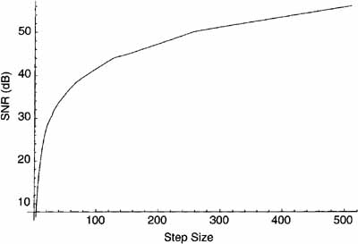
The SNR can be found from Figures 9.7 and 9.8. The SMR is the output of the psychoacoustic model. Because step size is growing exponentially, Figure 9.7 has a logarithmic shape that doesn’t show the low values very well. Figure 9.8 shows just the low values of step size.
Figure 9.7 Signal-to-Noise versus Step Size
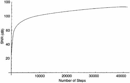
Figure 9.8 Signal-to-Noise versus Step Size (for Small Step Sizes)
The number of bits for (1) the samples “bspl”, (2) scalefactors “bscf”, and (3) Scalefactor Selection Information “bsel” are set to zero. The minimum MNR is increased by using the next higher index in the previous Possible Quantization per Subband section and a new MNR of this subband is calculated.
The number of bits for samples, bspl, is updated according to the additional number of bits required. If a nonzero number of bits is assigned to a subband for the first time, bsel and bscf have to be updated. Then adb is calculated again using the formula:
![]()
The iterative procedure is repeated as long as adbnext is not less than any possible increase of bspl, bsel, and bscf within one loop.
Quantization and Encoding of Subband Samples
The quantized sample Q(i) is calculated by
![]()
where the X(i) are the subband samples. A and B are determined with the following algorithm:
1. There are 17 indices. The first 14 are the same as noted previously under the Possible Quantization section. For indices 15-17, the value is 2i-1 – 1.
2. The A values for an index are the index value divided by the minimum power of 2 that is larger than the index value. For example, take index value 9. The next higher power of 2 is 16. The A value is then 9/16 = .5625.
3. The B values are all negative. The values can be calculated as follows: The denominator is 2number of bits to rePresent the index. The numerator is the denominator minus the index. For example, consider index 9. The bits required to represent 9 are 4 and 24 = 16. Thus, the denominator is 16. The numerator is then 16 – 9 = 7, and the value is -7/16 = -.4375.
N represents the necessary number of bits to encode the number of steps. The inversion of the MSB is done in order to avoid the all ‘1’ code that is used for the synchronization word.
The algorithm of the Possible Quantization section on page 187 shows whether grouping is used. The groups of three samples are coded with individual codewords if grouping is not required.
The three consecutive samples are coded as one codeword if grouping is required. Only one value vm, MSB first, is transmitted for this triplet. The empirical rule for determining vm (m = 3, 5, 9) from the three consecutive subband samples x, y, z is:
![]()
![]()
![]()
9.3.4 Formatting
The formatting for Layer II packets is given in Figure 9.9.
Figure 9.9 Layer II Packet Format Adapted from ISO Standard 11172-3, Figure C.3.

9.4 The Audio Decoding Process
To start the decoding process, the decoder must synchronize itself to the incoming bitstream. Just after startup this may be done by searching in the bitstream for the 12-bit syncword.
9.4.1 General
In DBS a number of the bits of the header are already known to the decoder, and, thus, can be regarded as an extension of the syncword, thereby allowing a more reliable synchronization. For Layer II, the number of bytes in a packet is
![]()
For DBS,
![]()
For DBS, the mode bits are ‘01’ for the intensity_stereo and the mode_ extension bits apply. The mode_extension bits set the bound, which indicates which subbands are coded in joint_stereo mode.
A CRC checkword has been inserted in the bitstream if the protection_ bit in the header equals ‘0’.
9.4.2 Layer II Decoding
The Audio decoder first unpacks the bitstream and sends any ancillary data as one output. The remainder of the output goes to a reconstruction function and then to an inverse mapping that creates the output left and right audio samples.
Audio Packet Decoding
The parsing of the Audio packet is done by using the following three-step approach.
1. The first step consists of reading “nbal” (2,3, or 4) bits of information for one subband from the bitstream. These bits are interpreted as an unsigned integer number.
2. The parameter nbal and the number of the subband are used as indices to compute nlevels that were used to quantize the samples in the subband.
3. The number of bits used to code the quantized samples, the requantization coefficients, and whether the codes for three consecutive subband samples have been grouped into one code can be determined.
The identifier sblimit indicates the number of the lowest subband that will not have bits allocated to it.
Scalefactor Selection Information Decoding
There are three equal parts (0,1,2) of 12 subband samples each. Each part can have its own scalefactor. The number of scalefactors that has to be read from the bitstream depends on scfsi[sb]. The Scalefactor Selection Information scfsi[sb] decodes the encoding shown in the Coding of Scalefactors section earlier in this chapter.
Scalefactor Decoding
The parameter scfsi[sb] determines the number of coded scalefactors and the part of the subband samples they refer to. The 6 bits of a coded scalefactor should be interpreted as an unsigned integer index. The Possible Quantization of Subbands section on page 187 gives the scalefactor by which the relevant subband samples should be multiplied after requantization.
Requantization of Subband Samples
The coded samples appear as triplets. From the Possible Quantization section, it is known how many bits have to be read for each triplet for each sub-band. As determined there, it is known whether the code consists of three consecutive separable codes for each sample or of one combined code for the three samples (grouping). If the encoding has employed grouping, degrouping must be performed. If combined, consider the word read from the bitstream as an unsigned integer, called c. The three separate codes—s[0], s[l], s[2]—are calculated as follows:

2 Note: (1) DIV is defined as integer division with truncation towards; and (2) nlevels is the number of steps, as shown in the Possible Quantization per Subband section.
To reverse the inverting of the MSB done in the encoding process, the first bit of each of the three codes has to be inverted. The requantized values are calculated by
![]()
s‴ = the fractional number
s′ = the requantized value
To calculate the coefficient C (not the Ci used in the Analysis Filterbank), let n equal the number of steps. Then,
![]()
where j is the smallest number of bits that can represent n. For example, if n = 9, then j = 4, since 4 bits are required to represent 9. Then,
![]()
The parameter D (not the Di used in the Synthesis Filterbank) can be calculated by
![]()
where j is the number of bits required to represent n. For example, if n = 31, j = 5, and
![]()
If the number of steps is 5 or 9, D = .5. If the number of steps is 3, 5, or 9, there is a grouping and the samples per codeword is 3; otherwise, there is no grouping and the samples per codeword is 1. The bits per codeword equals j, except where the number of steps is 3, 5, or 9, where the bits per codeword are 5, 7, and 10, respectively.
The parameters C and D are used in Equation (9.28). The requantized values have to be rescaled. The multiplication factors can be found in the calculation of scalefactors as described previously. The rescaled value s’ is calculated as:
![]()
Synthesis Subband Filter
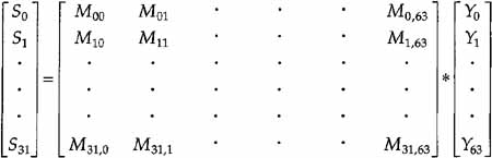
If a subband has no bits allocated to it, the samples in that subband are set to zero. Every time the subband samples for all 32 subbands of one channel have been calculated they can be applied to the synthesis subband filter and 32 consecutive audio samples can be calculated. For that purpose, the actions shown in the following algorithm detail the reconstruction operation.
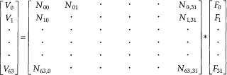
The coefficients Nik for the matrixing operation are given by
![]()
The coefficients Di for the windowing operation can be found from Figure 9.2. One frame contains 36 * 32 = 1,152 subband samples, which create (after filtering) 1,152 audio samples.
Synthesis Filterbank Algorithm
1. Input 32 new subband samples
2. Using these samples, perform the matrix multiply
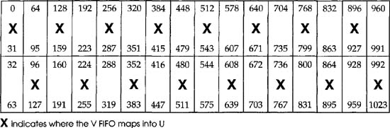
Sixteen of these V vectors are shifted into the FIFO shown here. Perform V into U mapping.
4. Window the U vector into a W vector by
![]()
5. Calculate the Output Audio samples