Chapter Thirteen: More Modeling Techniques and Commands
Chapter Objectives
Introduction
In addition to the primary methods involved in 3D solid modeling, AutoCAD has numerous other commands and techniques that facilitate the creation of particular 3D shapes. These include commands that produce regular 3D solid primitives, such as cones and spheres, commands that allow you to create 3D objects by revolving or extruding 2D outlines of 3D objects, and commands that create mesh models that can be shaped in ways that solids cannot. The addition of these techniques will make it possible for you to create all kinds of 3D models you cannot create with solid primitives. As we explore these new possibilities, we will also use the 3D Modeling workspace.
Polysolid |
|
|---|---|
Command |
Polysolid |
Alias |
(none) |
Panel |
Modeling |
Tool |
|

Drawing Polysolids
Most of this chapter is devoted to introducing commands for drawing shapes other than boxes, wedges, and cylinders. Some are created as simple solid primitives; others are derived from previously drawn meshes, lines, and curves. In this first section we draw a polysolid. Polysolids are drawn just like 2D polylines, but they have a height as well as a width. Like polylines, they can have both straight line and arc segments. Ours will include both.
polysolid: A 3D entity similar to a 2D polyline, but with the dimension of height added along with width and length.
✓ Create a new drawing using the acad3d template.
✓ Open the Workspace list from the status bar, and select 3D Modeling workspace from the list, if necessary.
Drawing in Multiple Tiled Viewports
A major feature needed to draw effectively in 3D is the ability to view an object from several different points of view simultaneously as you work on it. Here we introduce a three-viewport configuration so that you can see what is happening from different viewpoints simultaneously. If you do not continually examine 3D objects from different points of view, it is easy to create entities that appear correct in the current view but are clearly incorrect from other points of view. As you work, remember that these viewports are simple model space tiled viewports. Tiled viewports cover the complete drawing area, do not overlap, and cannot be plotted simultaneously. Plotting multiple viewports is accomplished in paper space layouts with floating viewports.
tiled viewports: Viewports that cover the drawing area and do not overlap. Tiled viewports may show objects from different points of view, but are not plotted.
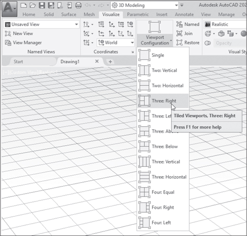
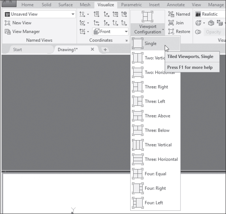
✓ Pick the Visualize tab > Viewport Configuration drop-down list > Three: Right from the ribbon, as shown in Figure 13-1.
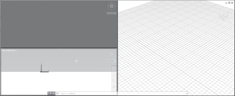
You now see three viewports, as shown in Figure 13-2. Currently each viewport displays the same 3D point of view, as you can verify by clicking in each viewport in succession to make it active. You find that all three show the same viewpoint, but only the active viewport shows the model, the navigation bar, the viewport label, and the USC icon.

We alter each viewport to achieve the views we want to work in. For this we use the Views list shown in Figure 13-3.

Notice also the very small gray sliders in the middle of each viewport border. These can be used to adjust the boundaries among the three viewports. Try it if you like. By clicking one of these sliders you can move the border line horizontally or vertically between any two adjacent viewports.
✓ Make sure that the right, 3D viewport is the active viewport, as it should be by default.
✓ From the Visualize tab, Named Views panel, open the View Manager, select SE Isometric, and click the Set Current button, as shown in Figure 13-3.
✓ Click Ok to leave the View Manager.
AutoCAD changes to a higher angle as shown in the right viewport in Figure 13-4.
✓ Click in the upper left viewport to make it active.
✓ Open the View Manager again and select Top.
✓ Click Ok to leave the View Manager.
✓ Click in the lower left viewport to make it active.
✓ Open the View Manager again and select Front.
✓ Click Ok to leave the View Manager.
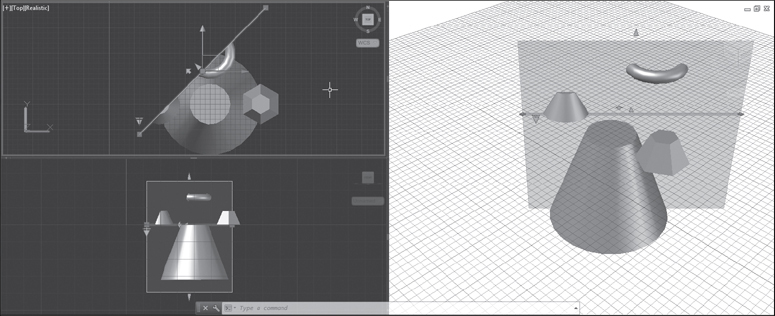
Your screen should now resemble Figure 13-4. The view on the right is a southeast isometric view. The top left viewport is a plan view, and the bottom viewport shows a front view. These viewpoints are labeled in the upper left corner of each viewport when that viewport is active. The front view has a different UCS from the views in the other two viewports. The coordinate system has been rotated so that the Z-axis still points out of the screen. If the UCS in this viewport were the same as the others, the Y-axis would be pointing out of the screen, and the Z-axis would be vertical in the plane of the screen. Because you would be looking in along the XY plane, you would have no ability to use the cursor in this viewport. Still, the change in color in this viewport shows the horizon in the world coordinate system even though the axes are rotated 90°.
✓ Click in the right viewport to make it active.
✓ Turn on Snap Mode and Ortho Mode.
We are now ready to begin drawing in this viewport configuration. Once you have defined viewports, any drawing or editing in the active viewport appears in all the viewports. As you draw, watch what happens in all viewports. You may need to zoom out or pan to get full views in each viewport.
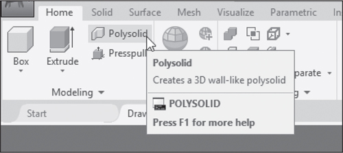
✓ Pick the Home tab > Modeling panel > Polysolid tool from the ribbon, as shown in Figure 13-5.
AutoCAD prompts:
POLYSOLID specify start point or [Object Height Width
Justify] <Object>:
To ensure your polysolid looks like ours, we will specify a height.
✓ Select Height from the command line.
✓ Type 4 <Enter> for the height.
AutoCAD returns the original prompt.
✓ Pick point (2.5,2.5,0) for a start point.
AutoCAD shows you a polysolid to drag. It will appear like a wall in the 3D viewport and can be stretched out, like drawing a line segment. With Ortho on it will stretch only orthogonally. AutoCAD prompts for the next point.
✓ Pick the point (10,2.5,0) for the next point.
Notice that this makes this segment 7.5 units long. From here, you could continue to draw straight segments, but we switch to an arc.
✓ Right-click and select Arc from the shortcut menu.
AutoCAD shows an arc segment and prompts for an endpoint. With Ortho on you can stretch in only two directions.
✓ Pick the point (10,8,0) for the arc endpoint.
Now, we switch back to a line segment.
✓ Right-click and select Line from the shortcut menu.
AutoCAD shows a straight segment beginning at the endpoint of the arc and prompts for a next point.
✓ Pick the point (2.5,8,0) for the next point. Again this is a length of 7.5 units.
Finally, we will switch to arc again and then use the Close option to complete the polysolid.
✓ Right-click and select Arc from the shortcut menu.
✓ Type c <Enter> to close.
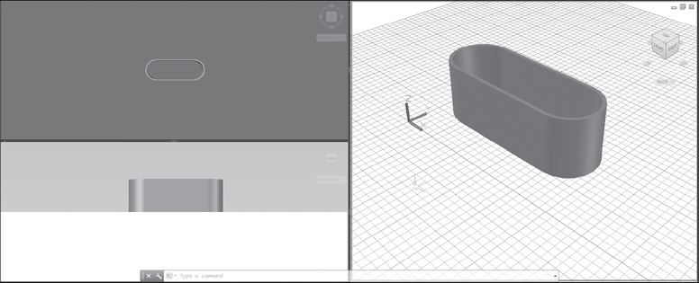
Your screen should resemble Figure 13-6.
Drawing Cones
Solid Cone Primitives
Cones are easily drawn by specifying a base and a height. The CONE command can also be used to draw flat-topped cones, called frustum cones, as we do in a moment.
frustum cone: A cone that does not rise to a point. It has a bottom radius and a top radius and is therefore flat-topped.
Cone |
|
|---|---|
Command |
Cone |
Alias |
- |
Panel |
Modeling |
Tool |
|

✓ Erase the polysolid from the “Drawing Polysolids” section.
✓ Pick the Cone tool from the Solid Primitives drop-down list on the Modeling panel, as shown in Figure 13-7.
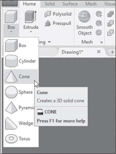
Notice that this is the same drop-down list as in the 3D Basics workspace. AutoCAD prompts:
Specify center point of base or [3P 2P Ttr Elliptical]:
Notice the other options, including the option to create cones with elliptical bases.
You can specify the base in either the top viewport or the right viewport. Using the top viewport will give you a better view of the base and its coordinates.
✓ Click in the top left viewport to make it active.
✓ Turn on Snap Mode in this viewport.
✓ Pick point (5,5,0) for the center of the cone base.
AutoCAD prompts:
Specify base radius or [Diameter] <0.0000>:
✓ In the top left viewport show a radius of 2.
AutoCAD draws a cone in each viewport and prompts for a height:
Specify height or [2P Axis endpoint] <0.0000>:
✓ Move the cursor and observe the cones in each viewport.
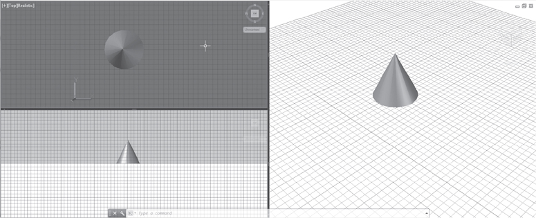
If you look carefully, you will notice that the cone in the top viewport appears to tilt slightly to the left. This viewport is drawn in perspective projection. The tilt effect is a result of the perspective projection. The other viewports show that there is no actual tilt. The perspective projection can cause some problems in plan views such as the upper left viewport. We will fix this later in the “Drawing Torus” section.
✓ Pick a point to indicate a height of 4.
The cone is complete, and your screen will resemble Figure 13-8.
Frustum Cones
Next, we create a cone with a negative z height and a different top radius. Cones with different top and bottom radii (that do not rise to a point) are called frustum cones.
✓ Pick the Cone tool from the Modeling panel.
✓ In the top left viewport, pick the point (10,5,0) for the base center.
✓ As before, show a radius of 2.
Move the cursor, and observe the cones in each viewport. We want to create a cone that drops down below the XY plane. Notice that we cannot do this in the active top view.
✓ Click in the right viewport to make it active.
✓ Drag the cone downward, and notice the effects in the right viewport.
We also want this cone to have a flat top, so we need to specify this before specifying the height.
✓ Right-click and select Top Radius from the shortcut menu.
AutoCAD prompts:
Specify top radius <0.0000>:
Move the cursor again to see the range of possibilities. You can create anything, from a very large, wide, flat cone to a long, narrow one. The top radius can be larger or smaller than the base radius. Also, the top can be below the base.
✓ Type 5 <Enter> for a top radius.
AutoCAD prompts again for a height.
✓ Make sure the right viewport is showing the cone in the negative direction, and type 8 <Enter> for a height.
Your screen should resemble Figure 13-9.

Drawing Pyramids
Drawing pyramids is much like drawing cones. Instead of a circular base, pyramids will have polygons at the base and possibly at the top. The process for drawing the base polygon is similar to using the POLYGON command.
Pyramid |
|
|---|---|
Command |
Pyramid |
Alias |
Pyr |
Panel |
Modeling |
Tool |
|

✓ Pick the Pyramid tool from the Solid Primitives drop-down list on the Modeling panel.
AutoCAD prompts:
Specify center point of base or [Edge Sides]:
The default is a four-sided base. We will opt for six sides.
✓ Right-click and select Sides from the shortcut menu, or select Sides from the command line.
AutoCAD prompts for the number of sides.
✓ Type 6 <Enter>.
AutoCAD takes this information and repeats the initial prompt. If you pick a center point, it will then prompt for the radius to the midpoint of a side, using the default Inscribed option. Recall that for an inscribed polygon the radius will be measured from the center to the midpoint of a side; for a circumscribed polygon the radius will be drawn out to a vertex. We proceed with the default Inscribed option.
✓ Pick (15,5,0) for the center point.
AutoCAD prompts for a base radius. The radius will be measured from the center point to the point you pick.
Note
By default, pyramids are drawn inscribed. If for any reason you have Circumscribed as your default you can switch by picking Circumscribed from the command prompt. The default will switch to Inscribed. This also works in reverse. Picking Inscribed from the command prompt will switch the option to Circumscribed.
✓ Pick the point (17,5,0) to show a radius of 2.
AutoCAD draws the base and prompts for height.
✓ Make sure your screen shows the pyramid in the positive direction, and type 4 <Enter>.
Your screen should resemble Figure 13-10.

Drawing Torus
Torus is another solid primitive shape that is easily drawn. It is like drawing a donut in 2D and requires an outer radius as well as a tube radius. Try this:
Torus |
|
|---|---|
Command |
Torus |
Alias |
Tor |
Panel |
Modeling |
Tool |
|

✓ Pick the Torus tool from the bottom of the Solid Primitives drop-down list on the Modeling panel.
AutoCAD prompts:
Specify center point or [3P 2P Ttr]:
The Three-point, Two-point, and Tangent Tangent Radius options work just as they do in the CIRCLE command. We will place a torus behind and above the frustum cone.
✓ Type 10,10,4 <Enter> for a center point.
Notice the z coordinate of 4, which places the torus above the XY plane.
AutoCAD prompts for a radius or diameter.
✓ Type 2 <Enter>.
Now, AutoCAD prompts for a second radius, the radius of the torus tube.
✓ Type .5 <Enter>.
Switching to Parallel Projection
Notice how the torus appears off center in the upper and lower left viewports. As mentioned previously, this is caused by the perspective projection. Having a perspective projection in a plan view is counterproductive. Here we switch to parallel projection in both of these viewports.
✓ Make sure that the upper left viewport is active.
✓ Right-click the ViewCube in the upper left viewport.
✓ Select Parallel.
Your upper left viewport should resemble the one in Figure 13-11. This figure also shows the lower left viewport in parallel projection. The same procedure will accomplish this.

✓ Make sure that the lower left viewport is active.
✓ Right-click the ViewCube in the lower left viewport.
✓ Select Parallel.
As shown, the lower left viewport is now in parallel perspective, and the horizon is no longer represented.
Slicing and Sectioning Solids
In addition to Boolean operations, there are other methods that create solid shapes by modifying previously drawn objects. In this section we explore slicing and sectioning.
Slice
The SLICE command allows easy creation of objects by cutting away portions of drawn solids on one side of a slicing plane. In this exercise we slice off the tops of a pyramid and a cone. For this purpose we will work in the front view in the lower left viewport.
Slice |
|
|---|---|
Command |
Slice |
Alias |
Sl |
Panel |
Solid Editing |
Tool |
|

✓ You should have the objects and viewports on your screen as shown in Figure 13-11 to begin this exercise.
✓ Click in the lower left viewport to make it active.
✓ Check to see that Snap Mode and Ortho Mode are on in this viewport.
✓ Pick the Slice tool from the Solid Editing panel, as shown in Figure 13-12.

AutoCAD prompts for objects to slice.
✓ Select the cone on the left and the pyramid on the right of the viewport.
✓ Right-click to end object selection.
AutoCAD prompts:
Specify start point of slicing plane or [planar Object/
Surface/Zaxis/View/XY/YZ/ZX/3points] <3points>:
This prompt allows you to define a plane by pointing, by selecting a planar object or surface of an object, or by using one of the planes of the current coordinate system. We can specify a plane with two points in the front view.
✓ Pick point (2.5,2,0) to the left of the cone.
✓ Pick point (17.5,2,0) to the right of the pyramid.
AutoCAD now has the plane defined but needs to know which side of the plane to cut.
✓ Pick a point below the specified plane.
The tops of the cone and pyramid will be sliced off, as shown in Figure 13-13.

Section
Sectioning is accomplished by creating a section plane and then picking options from a shortcut menu. Here we create a section plane through three of the objects on your screen and then create 3D section images.
✓ Click once in the top left viewport to make it active.
✓ If necessary, zoom out in this viewport so that all objects are completely visible within the viewport.
✓ Turn off Ortho Mode and Object Snap in this viewport, but leave Snap Mode on.
✓ Pick the Section Plane tool from the Section panel, as shown in Figure 13-14.
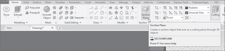
AutoCAD prompts:
Select face or any point to locate section line or [Draw
section/Orthographic]:
We begin by using point selection.
✓ Pick point (2.5,2.5,0).
AutoCAD shows a plane and prompts for a through point. We draw the plane through the middle of the cone and the torus.
✓ Pick point (12.5,12.5,0).
The section plane is drawn. Your screen should resemble Figure 13-15.

Adjust Section Plane with Grips
You now have three sectioned objects on your screen. They may be selected and modified independently. The section plane itself is also an object in your drawing and would be included if you plotted any of the three views represented. To plot the objects without the section plane, you can move the section plane to another layer and turn it off.
You can continue to adjust the location and effect of the plane by using grips. Here’s how:
✓ Make the top left viewport active and then select the section plane in this viewport.
A set of 3D grips and a gizmo will be added. The line used to create the plane will be highlighted, as shown in Figure 13-16. Grips will be added as shown in the top left viewport. These are also labeled in Figure 13-16. Taking these grips one at a time starting from the lower left, the first square grip is called the base grip. It is always adjacent to the menu grip, which is the second grip in our section plane view. The menu grip will give you a small set of sectioning options. By default, sectioning is cut along the plane, but you can also create two parallel planes to create a slice of the objects; a four-sided box, called a boundary, to slice the objects along four planes rather than one or two; or you can slice by specifying a volume for the remaining object.
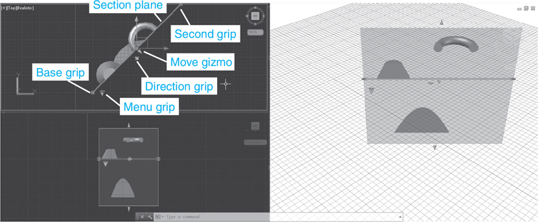
In the middle are two differently formed arrow grips. The first is a complete arrow with a small shaft. This is the direction grip. Selecting this grip will flip the geometry so that the opposite side of the plane is removed. The other arrow is a regularly shaped arrow grip, called simply the arrow grip. Picking, holding, and moving this grip will move the section plane in a direction normal to its current placement and will alter the sectioning of the object accordingly. The box grip at the intersection of the move gizmo is part of the gizmo and can be used to move the section plane according to standard gizmo editing procedures. Finally the square grip at the upper right is called the second grip. Ordinarily this grip will create rotation of the plane around the base grip at the other end. If you open the shortcut menu by right-clicking after picking the grip, you can choose other typical grip mode options.
Here we demonstrate three of these grip features, beginning with the direction grip. You are certainly invited to try out the others as well.
✓ With the plane selected, pick the direction grip near the middle of the section plane.
The sectioned geometry is immediately switched to the opposite side of the plane, as shown in Figure 13-17.
✓ Pick the direction grip again.
Sectioning flips back to the other side, shown previously in Figure 13-16.
Next we demonstrate the arrow grip in the middle of the plane.
✓ Pick the arrow grip, move the plane about 2 units to the right, and press the pick button again.
The section plane is moved orthogonally, and the objects are sectioned along a plane in its new location, as shown in Figure 13-18.
Finally, we use the second grip (at the top) to rotate the section around the base grip.
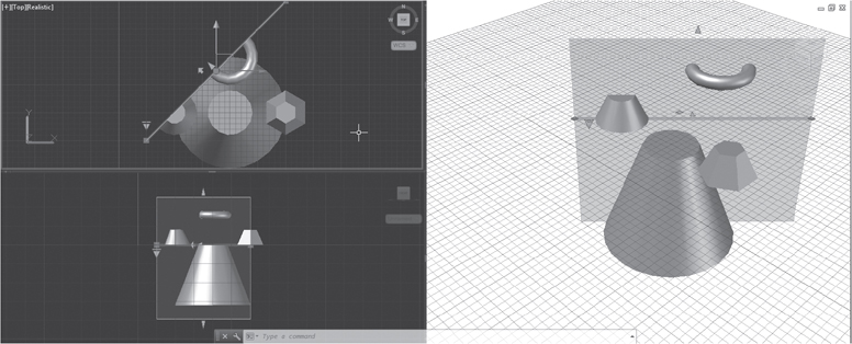
✓ Pick the second grip and move the cursor down to change the angle of the plane, as shown in Figure 13-19.

Your top viewport will resemble Figure 13-19.
Note: At times you may want to add a hatch pattern to highlight the sectioned surfaces. You can use the following procedure:
![]() Pick the small arrow at the right of the Section panel title on the Home tab in the 3D Modeling workspace. This opens a tall dialog box labeled Section Settings. The second section of this dialog box is labeled Intersection Fill. The second item under Intersection Fill is Face Hatch. By default this is set to Predefined/SOLID.
Pick the small arrow at the right of the Section panel title on the Home tab in the 3D Modeling workspace. This opens a tall dialog box labeled Section Settings. The second section of this dialog box is labeled Intersection Fill. The second item under Intersection Fill is Face Hatch. By default this is set to Predefined/SOLID.
![]() Click in the Face Hatch edit box and pick the list box arrow to the right of this setting to open the list.
Click in the Face Hatch edit box and pick the list box arrow to the right of this setting to open the list.
![]() Select Hatch Pattern type . . ..
Select Hatch Pattern type . . ..
![]() Pick the Pattern button to see images of different patterns, or open the drop-down list by picking the arrow to the right to open a list of pattern names.
Pick the Pattern button to see images of different patterns, or open the drop-down list by picking the arrow to the right to open a list of pattern names.
![]() Select a hatch pattern.
Select a hatch pattern.
![]() Pick OK if you are in the hatch pattern palette.
Pick OK if you are in the hatch pattern palette.
![]() Pick OK to close the Hatch Pattern Type dialog box.
Pick OK to close the Hatch Pattern Type dialog box.
![]() Pick OK to close the Section Settings dialog box.
Pick OK to close the Section Settings dialog box.
Mesh Modeling
Mesh modeling is a system that allows you to create free-form mesh solids with adjustable levels of smoothness to better represent real objects. This exercise takes you through a complete mesh modeling project, introducing many of the concepts, features, and procedures available in this system of 3D drawing.
mesh modeling: A 3D modeling system in which 3D mesh objects are created with faces that can be split, creased, refined, moved, and smoothed to create realistic free-form models.
✓ To begin, erase all objects from your screen, or begin a new drawing using the acad3D template.
✓ Zoom All.
✓ If you are in the drawing continued from the last section, return to a single viewport by making the right viewport active, and then selecting Visualize tab > Model Viewports panel > Viewport Configuration drop-down list > Single from the ribbon, as shown in Figure 13-20.
✓ If you are in a new drawing, pick Visualize tab > Named Views panel > View Manager > SE Isometric.
✓ Click Set Current and then OK to leave the View Manager.
This will take you to a higher angle necessary for some of the steps that follow.
✓ Pick the Mesh tab from the ribbon.
We begin by drawing a mesh cylinder. Mesh primitives are created just like solid primitives, but they can be edited very differently. Knowing what works with meshes and what works with solids is an important aspect of this type of drawing, as you will see.
✓ Turn on Grid Mode, Snap Mode, and Ortho Mode.
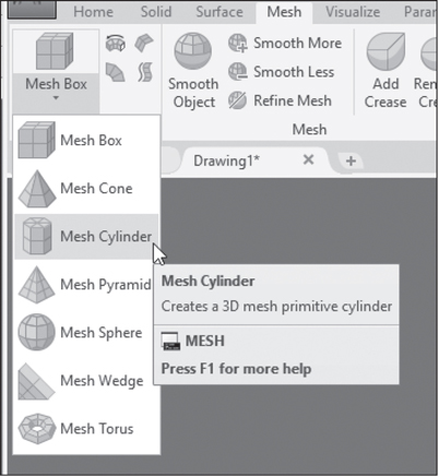
✓ Pick the Mesh Cylinder tool from the Mesh Primitives drop-down list, as shown in Figure 13-21.
✓ Pick (5,5,0) for the center point of the base.
✓ Stretch the cylinder out to show a radius of 2.5.
✓ Make sure that the cylinder is stretched in the positive Z direction and type 5 <Enter>.
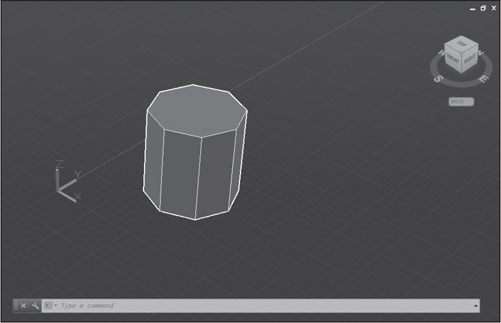
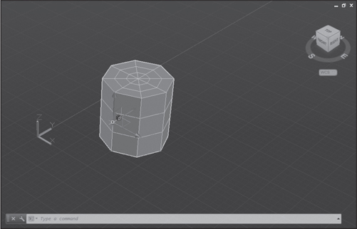
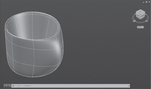
You have a complete mesh cylinder, as shown in Figure 13-22. Notice that the cylinder has distinct faces on all sides and that the presentation is faceted, instead of smooth and rounded, as a solid cylinder would be. The faces give us opportunities to shape and mold the object. Smoothness will be added later. In mesh modeling, we begin with faceted images that serve as an outline for the smooth object we wish to create. It will also be useful to use a visual style with edges visible.
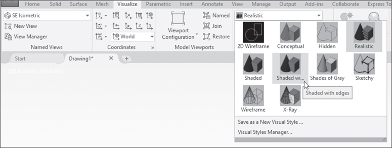
✓ Pick Visualize tab > Visual Styles drop-down list (not the Visual Styles panel extension) > Shaded with edges, as shown in Figure 13-23.
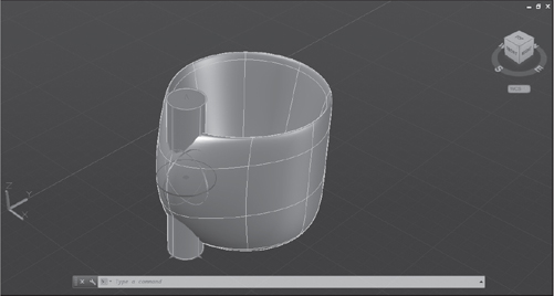
In this exercise we manipulate this cylinder to form the semblance of a stylized coffee mug. The first step is to pull an edge out away from the center to form the outline of a handle.
Subobject Filters
Looking at the mesh cylinder, you see that it is divided into faces. The faces meet at common edges, and at each corner of a face there is a vertex. These three elements, faces, vertices, and edges, are common to all meshes and are called subobjects. The importance of subobjects is that they can be selected individually or in groups for editing. When a subobject is moved, for example, its connections to other subobjects in the mesh are maintained, and the image is adjusted to accommodate the move.
subobject: In AutoCAD mesh modeling, a face, edge, or vertex that can be independently selected for editing.
To facilitate the selection of subobjects, the Mesh tab has a Filters drop-down list on the Selection panel. This list has tools for selecting only faces, only edges, or only vertices.
✓ Pick Home tab > Selection panel > Filters drop-down list > Edge, as shown in Figure 13-24.

To begin molding this cylinder into the shape of a mug, we select a single edge and move it outward.
✓ Move your cursor over the cylinder.
As you do this, you will see an edge icon added to the crosshairs and each edge you cross will be highlighted. Some of the edges will not be in the front of the cylinder as it is now positioned, so look carefully to see that the edge you want is selected.
For this exercise, it is important that you select the edge shown. This edge lies in the plane that is parallel to the YZ plane, which ensures we can use Ortho mode to get a clean, symmetrical result.
✓ With the middle front left edge selected, as shown, press the pick button.
✓ If necessary, pick the Move Gizmo tool from the Selection panel.
Your screen should resemble Figure 13-25.
Gizmos can be used to move, rotate, or scale subobjects as well as complete objects. In this case we will move the edge 1.5 in its plane parallel to the Y-axis.
✓ Rest your cursor on the Y-axis of the gizmo so that the green construction line is showing.
✓ With the Y-axis construction line showing, press and hold the pick button.
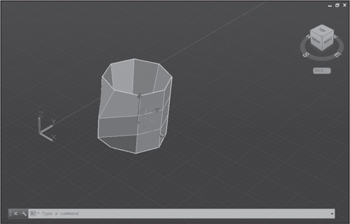
✓ Without releasing the pick button, stretch the edge out to the left, as shown in Figure 13-26.

✓ Still without releasing the pick button, type 1.5 <Enter>.
✓ Press <Esc> to remove the gizmo.
Your screen should resemble Figure 13-27.

Next, we select all the middle two rings of faces on the top of the cylinder and move them down 4.75 to create the inside of the mug.
✓ Pick the Face tool from the Filters drop-down list on the Selection panel.
Now as you move the cursor over the cylinder, faces will be highlighted instead of edges.
✓ Select each of the sixteen inner faces on the top of the cylinder, as shown in Figure 13-28.

As each face is selected with the pick button, a red dot appears, as shown.
Tip
If a gizmo gets in your way, pull down the gizmo list and select No Gizmo.
✓ If necessary, pick the Move Gizmo tool from the Selection panel.
✓ With the sixteen faces selected, move your cursor so that the vertical blue line on the Move Gizmo appears and the blue arrow turns gold.
✓ Press and hold the pick button.
✓ Without releasing the pick button, stretch the faces downward.
✓ Make sure that Ortho Mode is on; if it is not, press <F8>.
✓ With Ortho on and the faces stretched downward, type 4.75 <Enter>.
Notice how the outer faces stretch along their edges with the inner faces to maintain the connections, as shown in Figure 13-29.
To complete this object we smooth the mesh, convert it to a solid, and then subtract a cylinder to form a hole in the handle. The order in which we do things is important because of the limitations of both solids and meshes. Only mesh primitives can be smoothed, and only solids can be combined using Boolean operations. In a task like this one, we do all our subobject manipulation on the mesh primitive first; then we smooth the mesh. Finally, we convert the mesh to a solid so that we can do a subtraction. Although it is possible to convert either way, a solid converted to a mesh will not have the same clearly organized structure of meshes found in a mesh primitive.
Having completed the structure of our mesh, we can now add smoothness.
Smoothing Meshes
Meshes can be presented with varying levels of smoothness. At each level, the overall outline is maintained, but the number of faces increases until all the faces blend into a smooth surface. Each added level multiplies the number of mesh faces by four. Adding smoothness is simple.
✓ Pick the Smooth More tool from the Mesh panel, as shown in Figure 13-30.

Your screen resembles Figure 13-31. Faces have been multiplied and diminished in size. Edges have been softened, and the object has a more rounded look. The darker lines show the original faces, but each original face is now divided into four faces.

✓ Pick the Smooth More tool again.
Your screen resembles Figure 13-32. The mesh is smoothed further. The number of faces has increased dramatically. Each original face is now divided into 16 faces. The appearance is much smoother, but the new divisions are still clearly visible on the faceted surfaces. We can smooth the mesh even more.

✓ Pick the Smooth More tool.
Your screen resembles Figure 13-33. It is still smoother, with still more faces. If you look closely you can see 8 × 8 patterns on each original face, 64 faces each. But these faces are still distinct and visible. We can go one more level.

✓ Pick the Smooth More tool.
Your screen resembles Figure 13-34. You can no longer see or count the divided faces. The edge lines still show the original faces, but we have reached the fourth and final level of smoothness. If we attempt to go further, we get a message that says: “One or more meshes in the current selection cannot be smoothed again.”

Boolean Operations on Meshes and Solids
Next, we draw a solid cylinder and subtract it from the mesh to create a hole in the handle. To accomplish this, we also need to convert the mesh to a solid. Only meshes can be smoothed; only solids can be combined through the Boolean operations. Although we could draw the cylinder in the current view, procedures will be much clearer and more reliable if we temporarily change to a plan view. We use the ViewCube and move in two steps. First we move our viewpoint over to the southwest isometric. This view is also called the “home” view because it puts us directly over the origin of the world coordinate system.
✓ Move your cursor over the ViewCube so that the small house icon appears above the cube, as shown in Figure 13-35.
✓ Pick the house icon.
This moves your viewpoint so that your screen resembles Figure 13-36. Notice the red X-axis and the green Y-axis that converge off the screen in the direction from which you are looking, putting you roughly at the origin.
The second step is to move to a top, or plan, viewpoint.
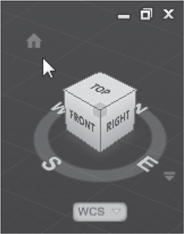
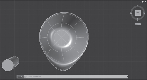
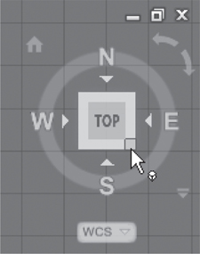
✓ Move your cursor over the Top face of the ViewCube, and press the pick button, as shown in Figure 13-37.

Your screen resembles Figure 13-38. This is a standard plan view in the WCS, with the X- and Y-axes aligned with the sides of the display. We draw a 1.0-diameter solid cylinder at (0,2.5), move it into the handle, rotate it, and subtract it to complete our drawing. So far in this exercise we have been working with a mesh object. From here on we will work with solids.

✓ Pick the Home tab on the ribbon.
Remember that the Home tab has solid modeling tools, whereas the Mesh tab has mesh modeling tools.
✓ Pick the Cylinder tool from the Solid Primitives drop-down list on the Modeling panel.
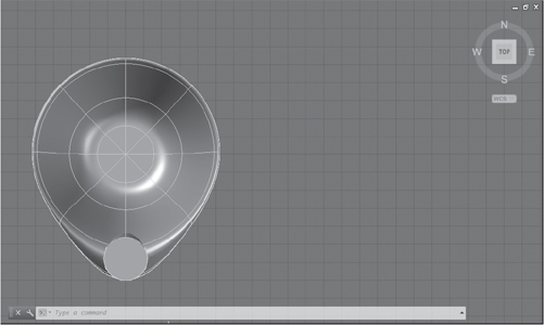
✓ Pick (0,2.5,0) for the center of the base, as shown in Figure 13-39.
✓ Pick a radius point 0.50 from the center of the cylinder.
✓ Type 5 <Enter> for the cylinder height.
Next, we move the cylinder 5 units to the right to center it within the stretched portion of the mesh.
✓ Pick the Move Gizmo from the Selection panel.
✓ Pick No Filter from the Filter drop-down list (to the left of the Gizmo drop-down).
✓ Select the solid cylinder.
✓ Move the cursor to highlight the red X-axis on the Move Gizmo.
✓ Press and hold the pick button.
✓ Drag the cylinder to the right.
✓ Without releasing the pick button, type 5 <Enter>.
✓ Press <Esc> to remove the gizmo.
Your screen resembles Figure 13-40. For the next step, we return to the southeast isometric view.
✓ Pick the southeast corner of the ViewCube, as shown in Figure 13-41.
Your screen resembles Figure 13-42. To rotate the cylinder 90°, we switch to the Rotate gizmo.

✓ Open the Gizmo drop-down list on the Selection panel and pick the Rotate Gizmo tool.
✓ Select the solid cylinder.
✓ Move the cursor to highlight rotation in the green XZ plane, around the Y-axis, as shown in Figure 13-43.
✓ Press the pick button and type 90 <Enter>.
✓ Press <Esc> to remove the gizmo.
Your screen resembles Figure 13-44.

Converting Meshes to Solids
Before we can subtract the solid cylinder from the smoothed mesh, we have to convert the mesh to a solid. This process is simplified by initiating the subtraction first. Before AutoCAD performs the subtraction, it will give us the option of converting the mesh to a solid. Conversion is simple, but you should not convert until you are sure that you are satisfied with the shaping of the mesh. If you attempt to convert back to a mesh, the mesh created will not be well organized and will be difficult to shape.
✓ Pick the Home tab > Solid Editing panel > Subtract tool from the ribbon.
✓ Select the mesh object.
✓ Right-click to end object selection.
AutoCAD presents the message shown in Figure 13-45. You have three choices of what to do with the mesh objects in your selection set.

✓ Select the middle option, Convert selected objects to smooth 3D solids or surfaces.
AutoCAD prompts for objects to subtract.
✓ Select the solid cylinder.
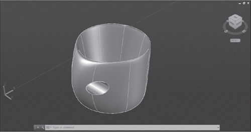
✓ Right-click to end object selection.
Your screen should resemble Figure 13-46. This is a simple but effective model. To achieve more realism and more definition, consider that faces can be split and creases added before editing. Creased edges retain their positions when adjacent faces are moved. By adding creases and additional faces to the edges on both sides of the handle, for example, you could create a narrower, more finely shaped handle.
Adjusting Viewpoints with 3DORBIT
Orbit
The 3DORBIT command is a dramatic method for adjusting 3D viewpoints and images. 3DORBIT has many options and works in three distinct modes. We begin with Orbit and then explore Free Orbit and Continuous Orbit. The standard views such as the top, front, and isometric views found on the ViewCube are generally all you need for the creation and editing of objects, and sticking with these views keeps you well-grounded and clear about your position in relation to objects on the screen. However, when you move from drawing and editing into presentation, you find 3DORBIT vastly more satisfying and freeing than the static viewpoint options.
3DORBIT |
|
|---|---|
Command |
3Dorbit |
Alias |
3do |
Panel |
Navigate |
Tool |
|

The model created in the last section will work well for a demonstration of 3DORBIT.
✓ Click the arrow beneath the Orbit tool on the navigation bar to open the list shown in Figure 13-47.

If for any reason your navigation bar has been turned off, turn it on by typing navbar <Enter> and selecting On from the command line.
✓ Pick Orbit, as shown.
Notice the orbit cursor that replaces the crosshairs.
✓ Press the pick button and slowly move the cursor in any direction.
The model moves along with the cursor movement.
✓ Move the cursor left and right, using mostly horizontal motion.
Horizontal motion creates movement parallel to the XY plane of the world coordinate system.
✓ Move the cursor up and down, using mostly vertical motion.
Vertical motion creates movement parallel to the Z-axis of the world coordinate system. You can create any viewpoint on the model using these simple motions. Notice also that the ViewCube moves in the same manner as the model.
✓ Move the cursor back to create a point of view similar to the one we started with.
✓ Press <Enter> to exit 3DORBIT.
Free Orbit
In Free Orbit mode, 3DORBIT makes use of a tool called an arcball, as shown in Figure 13-48. The center of the arcball is the center of the current viewport. Therefore, to place your objects near the center of the arcball, you must place them near the center of the viewport; or, more precisely, you must place the center point of the objects at the center of the display.

✓ If necessary, use Pan, or pan with the scroll wheel, to adjust the model so that it is roughly centered on the center of the viewport.
✓ Turn off Grid Mode.
Before entering 3DORBIT you can select viewing objects. 3DORBIT performance is improved by limiting the number of objects used in viewing. Whatever adjustments are made to the viewpoint on the selected objects are applied to the viewpoint on the entire drawing when the command is exited. In our case, we have just one object to view, so we can use the whole drawing.
✓ Pick Free Orbit from the Orbit drop-down list.
Your screen is redrawn with the arcball surrounding your model, as shown in Figure 13-48.
The Arcball and Rotation Cursors
The arcball is a somewhat complex image, but it is very easy to use once you get the hang of it. It also gives you a more precise handle on what is happening than the Orbit mode does. We already know that the center of the arcball is the center of the viewport, or the center of the drawing area in this case, because we are working in a single viewport. AutoCAD uses a camera–target analogy to explain viewpoint adjustment. Your viewpoint on the drawing is called the camera position. The point at which the camera is aimed is called the target. In 3DORBIT, the target point is fixed at the center of the arcball. As you change viewpoints you are moving your viewpoint around in relation to this fixed target point.
There are four modes of adjustment, which we take up one at a time. Each mode has its own cursor image, and the mode you are in depends on where you start in relation to the arcball. Try the following steps:
✓ Carefully move the cursor into the small circle at the left quadrant of the arcball, as shown in Figure 13-48.
When the cursor is placed within either the right or the left quadrant circle, the horizontal rotation cursor appears. This cursor consists of a horizontal elliptical arrow surrounding a small sphere, with a vertical axis running through the sphere. Using this cursor creates horizontal motion around the vertical axis of the arcball. This cursor and the others are shown in Figure 13-49.

✓ With the cursor in the left quadrant circle and the horizontal cursor displayed, press the pick button and hold it down.
✓ Slowly drag the cursor from the left quadrant circle to the right quadrant circle, observing the model and the 3D UCS icon as you go.
As long as you keep the pick button depressed, the horizontal cursor is displayed.
✓ With the cursor in the right quadrant circle, release the pick button.
You have created a 180° rotation. Your screen should resemble Figure 13-50.

✓ With the cursor in the right quadrant circle and the horizontal cursor displayed, press the pick button again and then move the cursor slowly back to the left quadrant circle.
✓ Release the pick button.
You have moved the image roughly back to its original position. Now, try a vertical rotation.
✓ Move the cursor into the small circle at the top of the arcball.
The vertical rotation cursor appears. When this cursor is visible, rotation is around the horizontal axis, as shown in the chart in Figure 13-49.
✓ With the vertical rotation cursor displayed, press the pick button and drag down toward the circle at the lower quadrant.
✓ This time, do not release the pick button but continue moving down to the bottom of the screen.
The viewpoint continues to adjust, and the vertical cursor is displayed as long as you hold down the pick button. Notice that 3DORBIT uses the entire screen, not just the drawing area. You can drag all the way down through the command line, the status bar, and the Windows taskbar.
✓ Spend some time experimenting with vertical and horizontal rotation.
Note that you always have to start in a quadrant to achieve horizontal or vertical rotation. What happens when you move horizontally with the vertical cursor displayed or vice versa? How much rotation can you achieve in one pick-and-drag sequence vertically? What about horizontally? Are they the same amount? Why is there a difference?
✓ When you have finished experimenting, try to rotate the image back to its original position, shown previously in Figure 13-48.
If you are unable to get back to this position, don't worry. We show you how to do this easily in a moment. Now let's try the other two modes.
✓ Move the cursor anywhere outside the arcball.
With the cursor outside the arcball you can see the roll icon, the third icon in the chart in Figure 13-49. Rolling creates rotation around an imaginary axis pointing directly toward you out of the center of the arcball.
✓ With the roll icon displayed, press the pick button and drag the cursor in a wide circle well outside the circumference of the arcball.
Notice again that you can use the entire screen, outside of the arcball.
✓ Try rolling both counterclockwise and clockwise.
✓ Release the pick button and then start again.
Note that you must be in the drawing area with the roll icon displayed to initiate a roll and that you must stay outside the arcball.
Finally, try the free rotation cursor. This is the most powerful, and therefore the trickiest, form of rotation. It is also the same as the Orbit mode as long as you remain within the arcball. The free cursor appears when you start inside the arcball or when you cross into the arcball while rolling. It allows rotation horizontally, vertically, and diagonally, depending on the movement of your pointing device.
✓ Move the cursor inside the arcball and watch for the free rotation icon.
✓ With the free rotation icon displayed, press the pick button and drag the cursor within the arcball.
Make small movements vertically, horizontally, and diagonally. What happens if you move outside the arcball?
The free rotation icon gives you a less restricted type of rotation. Making small adjustments seems to work best. Imagine that you are grabbing the model and turning it a little at a time. Release the pick button and grab again. You may need to do this several times to reach a desired position.
✓ Try returning the image to approximate the southeast isometric view before proceeding.
Other 3DORBIT Features
3DORBIT is more than an enhanced viewpoint command. While you work within the command you can adjust visual styles, projections, and even create a continuous-motion effect. 3DORBIT options are accessed through the shortcut menu shown in Figure 13-51. We explore these from the bottom up, looking at the lower two panels and one option from the second panel.

You should remain in the 3DORBIT command to begin this section.
✓ Right-click anywhere in the drawing area to open the shortcut menu.
Preset and Reset Views
In the second from the bottom panel, there is a Preset Views option that provides convenient access to the standard ten orthographic and isometric viewpoints, so that these views can be accessed without leaving the command. Above this is a Reset View option. This option quickly returns you to the view that was current before you entered 3DORBIT. This is a great convenience, because you can get pretty far out of adjustment and have a difficult time finding your way back.
✓ Select Reset View from the shortcut menu.
Regardless of where you have been within the 3DORBIT command, your viewpoint is immediately returned to the view shown previously in Figure 13-48. If you have not left 3DORBIT, the view is reset to whatever view was current before you reentered the command. If you have attempted to return to this view manually using the cursors, you can see that there is still a slight adjustment to return your viewpoint to the precise view.
Visual Aids and Visual Styles
✓ Right-click to open the shortcut menu again.
On the bottom panel, you can see Visual Styles and Visual Aids selections. Highlighting Visual Aids opens a submenu with three options: Compass, Grid, and UCS icon. The Grid option is useful for turning the grid on and off without leaving the command. The Compass adds an adjustable gyroscope-style image to the arcball.
There are three rings of dashed ellipses showing the planes of the X-, Y-, and Z-axes of the current UCS. Try this if you like. We do not find it particularly helpful.
The third option on the submenu turns the 3D UCS icon on and off.
Highlighting Visual Styles opens a submenu with the ten 3D visual styles. We have been working in the Shaded with edges style. This allows you to change styles without leaving the command. Switching to Realistic, for example, would remove the edges that are left from the original face borders. Try it.
✓ Highlight Visual Styles and then select Realistic from the submenu.
Your model is redrawn without edges.
Continuous Orbit
Continuous orbit may not be the most useful feature of AutoCAD, but it is probably the most dramatic and the most fun. With continuous orbit you can set objects in motion that continues when you release the pick button.
✓ Right-click to open the shortcut menu again.
✓ Highlight Other Navigation Modes in the second panel.
This opens a submenu shown in Figure 13-52. We explore some of the Camera and Walk and Fly options in the “Walking Through a 3D Landscape” section. Continuous Orbit, like Free Orbit and Orbit (called Constrained Orbit on this menu), can also be initiated directly from the navigation bar. It actually executes a different command called 3DCORBIT.

✓ Select Continuous Orbit from the submenu.
The arcball disappears, and the continuous orbit icon is displayed, consisting of a sphere surrounded by two ellipses, as shown in Figure 13-53. The concept is simple: Dragging the cursor creates a motion vector. The direction and speed of the vector are applied to the model to set it in rotated motion around the target point. Motion continues until you press the pick button again.

✓ With the continuous orbit cursor displayed, press and hold the pick button, then drag the cursor at a moderate speed in any direction.
We cannot illustrate the effect, but if you have done this correctly, your model should now be in continuous rotation. Try it again.
✓ Press the pick button at any time to stop rotation.
✓ Press and hold the pick button again and drag the cursor in a different direction, at a different speed.
✓ Press the pick button to stop rotation.
✓ Press the pick button, drag, and release again.
Now, try changing directions without stopping.
✓ While the model is spinning, press and hold the pick button and drag in another direction.
Have a ball. Experiment. Play. Try to create gentle, controlled motions in different directions. Try to create fast spins in different directions. Try to create diagonal, horizontal, and vertical spins.
Tip
The best way to achieve control over continuous orbit is to pick a point actually on the model and imagine that you are grabbing it and spinning it. It is much easier to communicate the desired speed and direction in this way. Note the similarity between the action of continuous orbit and the free rotation or constrained orbit icon. The grabbing and turning are the same, but continuous orbit keeps moving when you release the pick button, whereas free rotation stops. Also notice that however complex your dragging motion is, continuous orbit registers only one vector, the speed and direction of your last motion before releasing the pick button.
One more trick before we move on:
✓ Set your model into a moderate spin in any direction.
✓ With your model spinning, right-click to open the shortcut menu.
The model keeps spinning. Many of the shortcut menu options can be accessed without disrupting continuous orbit.
✓ Select Reset View from the shortcut menu.
The model makes an immediate adjustment to the original view and continues to spin without interruption.
✓ Open the shortcut menu again.
✓ Highlight Visual Styles and select Conceptual.
The style is changed and the model keeps spinning—pretty impressive.
✓ To stop continuous orbit, press the pick button once quickly without dragging.
✓ Press <Enter>, <Esc>, or the spacebar to exit 3DCORBIT.
You return to the command prompt, but any changes you have made in point of view and visual style are retained.
Creating 3D Solids from 2D Outlines
In this chapter you have created several 3D solid primitives and one mesh model. In this section, we look at three commands that create 3D objects from 2D outlines. We explore extruding, revolving, and sweeping 2D shapes to create complex 3D objects.
extruding: A method of creating a three-dimensional object by projecting a two-dimensional object along a straight path in the third dimension.
Extrude
Extrude |
|
|---|---|
Command |
Extrude |
Alias |
Ext |
Panel |
Modeling |
Tool |
|

✓ To begin, erase all objects from your screen, or begin a new drawing using the acad3d template.
✓ Zoom All.
We begin by drawing a square and extruding it.
✓ Turn Snap mode on.
✓ Pick the Home tab > Draw panel > Rectangle tool from the ribbon.
✓ Pick the point (5.0,5.0,0) for the first corner.
✓ Pick the point (10.0,10.0,0) for the second corner.
✓ Pick the Extrude tool from the Modeling panel, as shown in Figure 13-54.
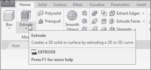
AutoCAD prompts for objects to extrude.
✓ Select the square.
✓ Press <Enter> to end object selection.
The EXTRUDE command will automatically convert the 2D square to a solid and give you an image to stretch in the positive or negative Z direction. The prompts also allow you to extrude in a direction other than along the Z-axis by drawing a directional line or using a preexisting line as a path.
We will use the Direction option to create a slanted solid.
✓ Select Direction from the command line.
AutoCAD prompts for the first point of a direction vector. The vector can be drawn anywhere.
✓ Pick the point (10,10,0) for the start point.
To place the endpoint above the XY plane, we use a point filter.
✓ At the prompt for an endpoint, type .xy <Enter> for an .XY point filter.
✓ At the of prompt, pick the point (10,12.5,0).
✓ At the need z prompt, type 2 <Enter>.
Your screen will resemble Figure 13-55. Before moving on to revolving, we demonstrate the technique of pressing and pulling solid objects.

Presspull
The PRESSPULL command allows you to extend a solid object in a direction perpendicular to any of its faces.
✓ Pick the Presspull tool from the Modeling panel, as shown in Figure 13-56.

AutoCAD prompts you to select a face. The prompt is:
Select object or bounded area:
✓ Pick the front face.
AutoCAD gives you an image to drag and a dynamic UCS with Z normal to the face.
✓ Pull in the positive and negative directions, perpendicular to the selected face.
✓ With the object pulled in the positive direction, type 3 <Enter>.
✓ Press <Enter> to exit the command.
Your screen should resemble Figure 13-57.

Revolve
The REVOLVE command creates a 3D solid by continuous repetition of a 2D shape along the path of a circle or arc around a specified axis. Here we draw a rectangle and revolve it 180° to create an arc-shaped model. Along the way we also demonstrate how a 2D object can be converted to a 3D planar surface.
Revolve |
|
|---|---|
Command |
Revolve |
Alias |
Rev |
Panel |
Modeling |
Tool |
|

Note
Coordinate systems can sometimes get out of order after a DUCS has been in use. To correct this, simply pick the World tool at the upper right corner of the Coordinates panel. This will return you to the world coordinate system.
✓ Pick the Rectangle tool from the Draw panel.
✓ Pick the point (15,5,0) for the first corner point.
✓ Pick the point (17.5,10,0) to create a 2.5 × 5.0 rectangle.
Next, we use the Convert to Surface tool to make this a rectangular surface rather than a wireframe outline. Note that this is for demonstration only. As in the EXTRUDE command, you can create a 3D solid directly from a 2D outline with the REVOLVE command.
✓ Pick the Home tab > Solid Editing panel extension > Convert to Surface tool from the ribbon, as shown in Figure 13-58.
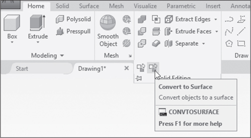
Notice that there is also a Convert to Solid tool, which will convert a model made of 3D surfaces to a solid model. AutoCAD prompts for object selection.
✓ Select the rectangle.
✓ Right-click to end object selection.
The rectangle will become a 3D surface, and your screen will resemble Figure 13-59.

✓ Pick the Home tab > Modeling panel > Extrude drop-down list > Revolve tool from the ribbon, as shown in Figure 13-60.

AutoCAD prompts for objects to revolve.
✓ Select the rectangular surface.
✓ Press <Enter> to end object selection.
AutoCAD gives several options for defining an axis of rotation:
Specify axis start point or define axis by [Object/X/Y/Z]
<Object>:
You can give start points and endpoints, select a line or polyline that has been previously drawn, or use one of the axes of the current UCS.
✓ Pick the point (20,0,0) for a start point.
✓ Pick the point (20,12.5,0) for an endpoint.
Next, AutoCAD needs to know how much revolution you want. The default is a full 360° circle.
Specify angle of revolution or [STart angle/Reverse/
EXpression] <360>:
Here we start at the horizon, 0°, and revolve through 180°, placing both ends of the arc on the XY plane.
✓ Select STart angle from the command line.
AutoCAD prompts for an angle.
✓ Press <Enter> to accept the default start angle, or type 0 if your angle has been changed.
AutoCAD now prompts for an angle of revolution.
✓ Type 180 <Enter>.
The revolved solid will be created and your screen will resemble Figure 13-61.

Helix
We have two more techniques to demonstrate before moving on. First, we use the HELIX command to create a 3D spiral outline. Then, we use the SWEEP command to convert the helix to a solid coil.
Helix |
|
|---|---|
Command |
Helix |
Alias |
(none) |
Panel |
Draw |
Tool |
|

✓ Pick the Helix tool from the Draw panel extension, as shown in Figure 13-62.

Helix characteristics can be changed using the Properties Manager. Among the default specifications are two shown in the prompt area. Number of turns will be the number of times the spiral shape goes around within the height you specify. The twist will be either counterclockwise or clockwise.
✓ Pick the point (12.5,–5.0,0) for the center point of the helix base.
AutoCAD prompts for a base radius:
Specify base radius or [Diameter] <1.0000>:
The default will be retained from any previous use of the command in the current drawing session.
✓ Pick a second point to show a radius of 2.5000.
AutoCAD now prompts for a top radius, showing that you can taper the helix to a different top height, similar to the options with the CONE and PYRAMID commands. We specify a smaller top radius.
✓ Type 1 <Enter> or pick a point to show a radius of 1.0000.
AutoCAD prompts for a height.
✓ Make sure the helix is stretched in the positive direction, and type 4 <Enter>.
The helix is drawn, as shown in Figure 13-63.

The SWEEP Command
Sweep |
|
|---|---|
Command |
Sweep |
Alias |
(none) |
Panel |
Modeling |
Tool |
|

Finally we sweep a circle through the helix path to create a solid coil.
✓ Pick the Circle Center, Radius tool from the Draw panel.
✓ Anywhere on your screen, create a circle of radius 0.5.
✓ Pick the Sweep tool from the Extrude drop-down list on the Modeling panel, as shown in Figure 13-64.
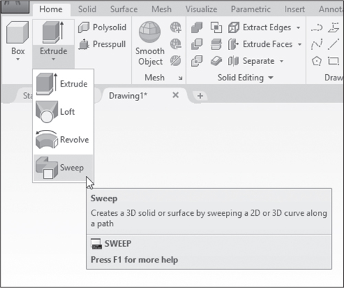
AutoCAD prompts for objects to sweep.
✓ Select the circle and press <Enter> to end object selection.
AutoCAD prompts:
Select sweep path or [Alignment/Base point/Scale/Twist]:
The default is to select a path, such as the helix. By default the object being swept will be aligned perpendicular to the sweep path. The Alignment option can be used to alter this. Base point allows you to start the sweep at a point other than the beginning of the sweep path. Scale allows you to change the scale of the objects being swept. By default the object being swept will remain perpendicular to the path at every point. To vary this and create a more complex sweep, use the Twist option. Here we use the default sweep path.
✓ Select the helix.
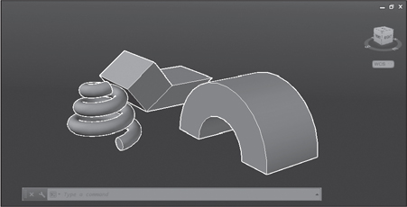
Your screen should resemble Figure 13-65.
That completes this section on modeling techniques. In the final two sections we demonstrate the use of CAMERA and WALK commands to move your point of view through the 3D landscape, and ANIPATH to create an animated walk-through.
Walking Through a 3D Landscape
AutoCAD has features that allow you to move your point of view through the 3D space of a drawing. This is useful in architectural drawings in which you can create a simulated walk-through of a model. In this section we demonstrate the use of the WALK command to navigate through the objects on your screen. The process involves creating a camera and a target and then using arrow keys to move the camera. Our goal to make it possible to navigate under the cylinder, as if we were walking under an arch.
Camera and Target
The first step will involve creating camera and target locations.
✓ To begin, you should be in a view similar to that shown previously in Figure 13-65.
✓ If necessary, turn on the grid.
✓ Pick Visualize tab > Camera panel > Create Camera tool from the ribbon, as shown in Figure 13-66.

AutoCAD prompts for a camera location. We will start with a location on the axis of the cylinder.
✓ Pick the point (20,–5), as shown by the camera icon in Figure 13-67.
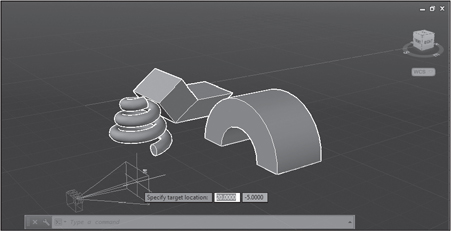
AutoCAD now prompts for a target location. In our case we want to point the camera along the axis of the cylinder. The distance to the target is not significant. AutoCAD shows the target with an image representing an expanding field of vision in the direction specified.
✓ Pick the point (20,0), as shown by the field of vision symbols in Figure 13-67.
AutoCAD shows you a set of options on the Dynamic Input menu in Figure 13-68. We choose the View option, which will change our display to align with the camera’s point of view on the target.

Tip
If you cannot see the View option, the Dynamic Input menu may be cut off at the bottom and covers the View option on the command line. If this happens, click once in any open section of the drawing area to move the menu.
✓ Select View from the command line or the Dynamic Input menu.
With another small menu, AutoCAD asks us to verify that we wish to switch to the camera view.
✓ Select Yes from the menu.
This completes the command and switches your view to the camera view shown in Figure 13-69. We are now ready to proceed with our walk.

The 3DWALK and 3DFLY Commands
The 3DWALK and 3DFLY commands use identical procedures, but 3DWALK keeps you in the XY plane, whereas 3DFLY allows you to move above or below the plane. Here we enter 3DWALK, walk through the arch, turn left to view the other objects, then turn around and walk back between the objects.
✓ Type 3dw <Enter>.
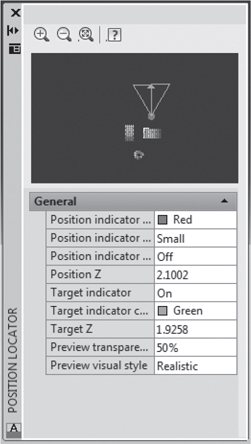
You see the Position Locator palette in Figure 13-70. This palette shows a plan view of the objects in the drawing with a red circle representing the camera position and a green triangle representing the target and field of vision. Before we begin to move through the view, it may be helpful to zoom out in the Position Locator to give us a little more room to work with.

✓ If necessary, click once on the Zoom in or Zoom out tool at the top of the Position Locator.
Your objects should appear smaller in the Position Locator, as shown in Figure 13-70. We use the forward arrow to move through the arch. Notice that AutoCAD also positions a green cross on the screen, indicating the target position.
✓ Press the up arrow key on your keyboard once to move forward.
You move a “step” closer to the arch. Notice also that the camera and target image move forward on the Position Locator palette.
✓ Continue pressing the up arrow and observing the screen image as well as the Position Locator.
✓ Walk through the arch until you reach the other side. Watch the Position Locator to ensure that you move the camera location completely through the arch.
At this point the camera location image on the Position Locator should be completely beyond the arch, as shown in Figure 13-71.
✓ Press the left arrow once and observe the Position Locator palette.
The camera and target image will shift to the left on the palette, and your viewpoint will shift in the drawing, but you will see no change because there is nothing but the horizon in this direction.
✓ Press the left arrow again.
Notice that the camera image continues to move to the left, but the target is still straight ahead.
✓ Continue moving to the left until the camera and target image is between the cylinder and the boxes to the left.
✓ Move the cursor over the arrow at the top of the green triangle representing the field of vision in the Position Locator.
When the cursor is in this position, it will appear with a hand icon, as used in the PAN command. With the hand icon showing, you can move and expand the field of vision.
✓ With the hand icon showing and resting on the field of vision triangle (not on the red “camera”), press and hold the pick button, and drag the triangle around 180°.
Your camera is now pointing toward the coil. Your screen should resemble Figure 13-72.

✓ Continue using the arrow keys and the mouse along with the pan cursor to move through the objects on your screen.
There is one other trick you should try. In addition to changing your field of vision in the Position Locator, you can change it directly in the drawing by dragging your mouse. Whereas moving the field of vision triangle will only create movement within the XY plane, the mouse can be moved up, down, sideways, and diagonally to view whatever objects are accessible from your current camera location. Try it.
✓ Press and hold the pick button, and drag the mouse right and left, up and down to view the objects in your drawing. As you do this, observe the changes in the field of vision triangle in the Position Locator palette.
✓ When you are done, press <Enter> to exit the command.
The objects will remain in whatever view you have created. Of course, you can return to your previous view using the U command.
Creating an Animated Walk-Through
The ability to walk through a landscape is impressive, but for presentation purposes it may be more important to have the walk-through animated so that any potential client can see the view without having to interact with AutoCAD in the ways you have just learned. Here we use the ANIPATH command to create a simple animation of a walk-through that is slightly different from the one we did manually in the last section. We begin by switching to a plan view.
✓ Select Visualize tab > Named Views panel > View Manager and then pick the Top view from the Views panel, as shown in Figure 13-73.

✓ Click Set Current and then OK.
Regardless of what was in your view previously, you should now be in the plan view shown in Figure 13-74.
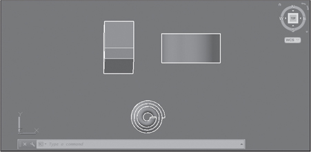
Animations follow paths specified by lines, polylines, or 3D polylines. For our purposes we will draw the simple polyline path shown in Figure 13-75. First, we will draw it with right angles and then fillet one corner, as shown.

✓ Pick the Home tab > Draw panel > Polyline tool from the ribbon.
✓ Pick the point (20,–5) for a start point.
✓ Pick the point (20,3.5) for the next point.
✓ Pick the point (12.5,3.5) for the next point.
✓ Pick the point (12.5,1.0) for the final point.
✓ Press <Enter> to complete the polyline and exit the command.
Now, we fillet the right corner to complete the path. The fillet will have a significant impact on the animation.
✓ Type F <Enter> or pick the Fillet tool from the Modify panel.
✓ Select Radius from the command line.
✓ Type 2 <Enter> for a radius specification.
✓ At the prompt for a first object, select the vertical line segment on the right.
✓ At the prompt for a second object, select the horizontal segment.
Your screen should resemble Figure 13-75.
We are now ready to create an animation.
✓ Type ani <Enter>.
This executes ANIPATH and opens the Motion Path Animation dialog box shown in Figure 13-76.

✓ In the dialog box, pick the Path button in the middle of the Camera panel, and then pick the Select button to its right.
The dialog box disappears, giving you access to the drawing area.
✓ Select the polyline.
The polyline is selected and AutoCAD asks for a Path Name, as shown in Figure 13-77.
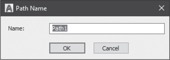
✓ Click OK to accept the default name (Path1).
This brings you back to the dialog box. We make one more critical adjustment.
✓ In the Animation settings panel on the right, change the Duration setting to 10.
If we did not change this setting, the animation would move very quickly, and it would be difficult to see what was happening.
✓ Make sure the When previewing show camera preview box is checked.
✓ Pick the Preview button at the bottom left of the dialog box.
AutoCAD shows you a preview of the path and then the actual animation preview. Watch closely. What you see will be an animation based on moving a camera along the specified path. Notice the difference between the gentle swing to the left along the fillet path and the abrupt left turn at the final right angle. When the animation is done, your Animation Preview box should resemble Figure 13-78. Closing the Preview takes you back to the dialog box, where you can continue to modify and preview the animation, or save it to a WMV file.
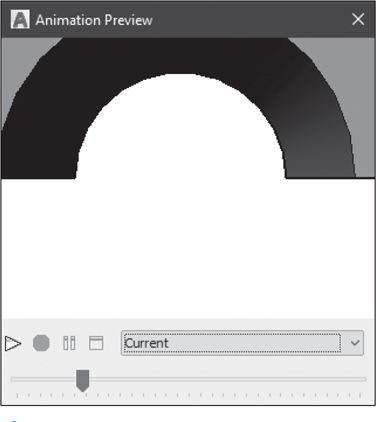
✓ Click the X in the upper right corner to close the Animation Preview.
This brings you back to the Motion Path Animation dialog box.
At this point you can cancel the animation and return to your drawing, or click OK to save it. If you click OK, AutoCAD will initiate a process of creating a video. It will be saved as a WMV file that can be played back by other programs such as Windows Media Player. Once created, you can run the video by opening the file and following the Windows Media Player procedure.
There you have it. Congratulations on your first video.
Chapter Summary
In this chapter you have learned to draw polysolids, cones, pyramids, torus, and mesh models, and to extrude 2D objects to form 3D solids. You can slice and section solids and convert 2D outlines into 3D solids and surfaces. You learned to use powerful tools for creating and adjusting 3D points of view and can present objects in continuous orbit. You learned to create a controlled walk-through of a 3D model and can record an animated walk-through for playback in AutoCAD or other media software.
Chapter Test Questions
Multiple Choice
Circle the correct answer.
1. Which of these cannot be extruded?
a. Line
b. Polysolid
c. Circle
d. Rectangle
2. Which of these is not a solid?
a. Extruded circle
b. Swept rectangle
c. Torus
d. Helix
3. In 3DWALK, the _______________ is always in the XY plane.
a. camera location
b. target location
c. field of vision
d. viewpoint
4. Unlike 3DWALK and 3DFLY, an animated walk-through requires a:
a. Camera
b. Target
c. Path
d. Gizmo
5. Mesh models should be converted to solid models:
a. Before editing
b. After changing visual styles
c. Before rendering
c. After smoothing
Matching
Write the number of the correct answer on the line.
a. Floating viewport ______ |
1. Solid primitive |
b. Tiled viewport ______ |
2. Not plotted |
c. Torus ______ |
3. Plotted |
d. Face ______ |
4. Subobject |
e. Arcball ______ |
5. 3DORBIT |
True or False
Circle the correct answer.
1. True or False: Tiled viewports are required for editing 3D models.
2. True or False: In a Three: Right viewport configuration, all three viewports are in parallel projection by default.
3. True or False: In a Three: Right viewport configuration, all three viewports are in plan view by default.
4. True or False: You can select the face of a solid box without a filter, but the filter makes it easier.
5. True or False: Only meshes can be smoothed; only solids can be combined.
Questions
1. Name at least three commands that create 3D models from 2D objects.
2. While still in the 3DORBIT command, what is the quickest way to return to the view you started with before entering 3DORBIT?
How do you access this feature without leaving the 3DORBIT command?
3. How many direction vectors are specified by the motion of your mouse in the Continuous Orbit mode?
4. What elements must be present in your drawing before you can use the 3DWALK and 3DFLY commands?
5. What additional element must be present before you can create an animated walk-through?
Drawing Problems
1. Beginning with a blank drawing using the acad3D template, draw a 0.5-radius circle anywhere on your screen.
2. Draw a helix with center point at (0,0,0), base radius 5.0, top radius 1.0, and height 5.0.
3. Sweep the circle through the helix path to create a solid coil. Erase the helix.
4. Draw a cone with base center at (0,0,0), radius 5.0, and height 6.5.
5. Subtract the coil from the cone.
6. Create a section view of the object; cut along the YZ plane.
Chapter Drawing Projects
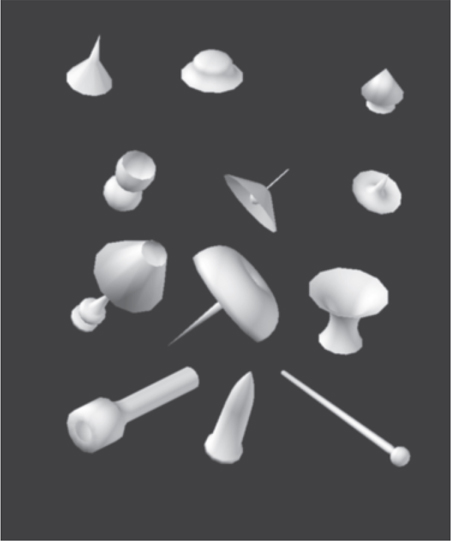
 Drawing 13-1: Revolve Designs [ADVANCED]
The REVOLVE command is fascinating and powerful. As you become familiar with it, you might find yourself identifying objects in the world that can be conceived as surfaces of revolution. To encourage this process, we have provided this page of 12 revolved objects and designs. The next drawing is also an application of the REVOLVE procedure.
To complete the exercise, you need only the PLINE and REVOLVE commands. In the first six designs, we have shown the path curves and axes of rotation used to create the designs. In the other six, you are on your own.
Exact shapes and dimensions are not important in this exercise, but imagination is. When you have completed our designs, we encourage you to invent your own. Also, consider adding materials and lights to any of your designs and viewing them from different viewpoints using 3DORBIT.

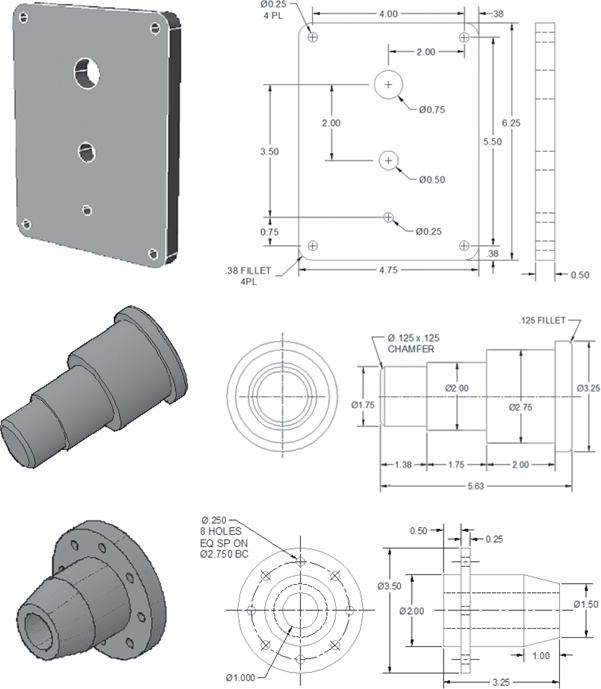
 Drawing 13-2: Tapered Bushing [ADVANCED]
This is a more technical application of the REVOLVE command. By carefully following the dimensions in the side view, you can create the complete drawing using PLINE and REVOLVE only.
Drawing Suggestions
Use at least two viewports with the dimensioned side view in one viewport and the 3D isometric view in another.
Create the 2D outline as shown and then REVOLVE it 270° around a centerline running down the middle of the bushing.
When the model is complete, consider how you might present it in different views on a paper space layout.

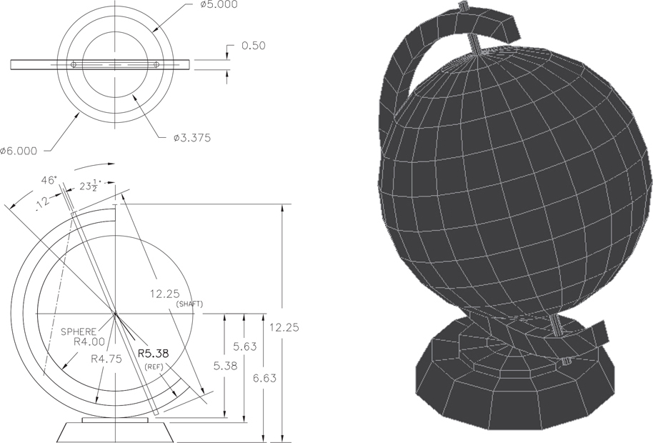
Drawing 13-3: Globe [ADVANCED]
This drawing uses a new command. The SPHERE command creates a 3D sphere, and you should have no trouble learning to use it at this point. You will find it on the Solid Primitives drop-down list on the Modeling panel. Like a circle, it requires only a center point and a radius or diameter.
Drawing Suggestions
Use a three-viewport configuration with top and front views on the left and an isometric 3D view on the right.
Use 12-sided pyramids to create the base and the top part of the base.
Draw the 12.25 cylindrical shaft in vertical position, and then rotate it around what will become the center point of the sphere, using the angle shown.
The arc-shaped shaft holder can be drawn by sweeping or revolving a rectangle through 226°. Considering how you would do it both ways is a good exercise. Then, choose one method, or try both.
As additional practice, try adding a light and rendering the globe as shown in the reference drawing.

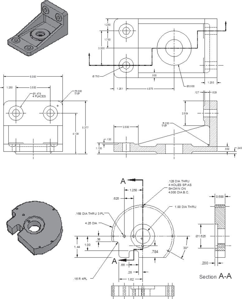
Drawing 13-4: Pivot Mount [ADVANCED]
This drawing gives you a workout in constructive geometry. We suggest you do this drawing with completely dimensioned orthographic views and the 3D model as shown. Also, create a sliced view of the model as shown in the reference figure.
Drawing Suggestions
Begin by analyzing the geometry of the figure. Notice that it can be created entirely with boxes, cylinders, and wedges, or you can create some objects as solid primitives and others as extruded or revolved figures. As an exercise, consider how you would create the entire model without using any solid primitive commands (no boxes, wedges, or cylinders). What commands from this chapter would be required?
When the model is complete, create the sliced view as shown.
Create the orthographic views and place them in paper space viewports.
Add dimensions in paper space.

Drawings 13-5 [ADVANCED]
The drawings that follow are 3D solid models derived from 2D drawings. You can start from scratch or begin with the 2D drawing and use some of the geometry as a guide to your 3D model.