This chapter covers basic probability concepts, reliability measures, fault tree (FT) modeling, binary decision diagrams (BDDs), and Markov processes. Some reliability analysis software tools are also introduced.

2.1 Basic Probability Concepts

Random experiment is an experiment with its outcome being unknown ahead of time but all of its possible individual outcomes being known [1]. The set of all possible outcomes of a random experiment constitutes its sample space, denoted by Ω. Each individual outcome in the sample space is referred to as a sample point.

A subset of a sample space associated with a random experiment is defined as an event that occurs if the experiment is performed and the outcome observed is in the subset defining the event. There are two special events: a certain event (sample space itself Ω) that occurs with probability ONE (1) and an impossible event (empty set ∅) that occurs with probability ZERO (0). Because events are sets, the operations in the set theory like complement, union, and intersection can be applied to generate new events.

If two events A and B do not share any common sample points, i.e. A ∩ B = ∅, then A and B are said to be disjoint or mutually exclusive.

2.1.2 Conditional Probability

Consider two events A and B. The conditional probability of event A given the occurrence of event B, denoted by P(A|B), is a number such that 0 ≤ P(A|B) ≤ 1 and P(A ∩ B) = P(B)P(A|B). In the case of P(B) ≠ 0, Eq. (2.1) presents a commonly used formula for evaluating the conditional probability.

(2.1)

If P(A ∩ B) = P(A)P(B), implying P(A|B) = P(A) and P(B|A) = P(B) (neither event influences the occurrence of the other event), then events A and B are said to be independent. Note that independence does not mean that the two events cannot share common sample points. In other words, two independent events are not necessarily two mutually exclusive events. Mutually exclusive events are independent only when at least one of them has ZERO occurrence probability.

2.1.3 Total Probability Law

A collection of events forms a partition of sample place Ω if it satisfies the following three conditions:

1. B_i ∩ B_j = ∅ for any i ≠ j;
2. P(B_i) > 0 for i = 1, 2, …, n;
3. .

Based on partition , for any event E defined on the same sample space Ω, its occurrence probability can be evaluated as

(2.2)

Equation (2.3) presents a special case of the total probability law since for any event B, B and form a partition of Ω.

(2.3)

2.1.4 Bayes' Theorem

Based on the total probability law and concept of condition probability, Bayes' theorem is

(2.4)

2.1.5 Random Variables

A random variable (r.v.) X is a real‐valued function, which maps each individual outcome ω in some sample space Ω to a real number , i.e. X: Ω → R.

A cumulative distribution function (cdf) F can be defined for X for a real number a as

(2.5)

The cdf F is a nondecreasing function, that is, if a < b then F(a) ≤ F(b). Also, for any a < b, P(a < X ≤ b) = F(b) − F(a).

A r.v. can be classified as discrete or continuous. A discrete r.v. can take on a countable number of possible values. In other words, the image of a discrete r.v. X is a finite or countably infinite subset of real numbers, denoted as T = {x₁, x₂, …}. Besides cdf, a discrete r.v. X can be characterized by a function called probability mass function (pmf) defined as

(2.6)

The pmf has the following properties: 0 ≤ p_X (a) ≤ 1 and .

A continuous r.v. can take on a range of uncountable real values. In general, the time when a particular event happens is a continuous r.v. Besides cdf, a continuous r.v. X can be characterized by a function called probability density function (pdf) defined as

(2.7)

The pdf f_X(x) is integrable and for any real numbers a < b, . For any real number a, . Also, .

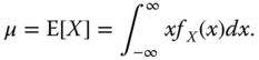
The mean (also known as expected value) of a r.v. represents the long‐run average of the variable or the expected average outcome over many observations. Equation (2.8) presents the formula calculating the mean of a discrete r.v. with pmf p_X (a).

(2.8)

Equation (2.9) presents the formula calculating the mean of a continuous r.v. with pdf f_X(x).

(2.9)

The variance of a r.v. measures its statistical dispersion, indicating how far its values typically are from the expected value. For a r.v. X with mean μ, the variance of X is defined by

(2.10)

Equation (2.11) presents an alternative formula for computing the variance of X.

2.11

The standard deviation of a r.v. is typically denoted by σ, which is simply the square root of the variance.

2.2 Reliability Measures

Several quantitative reliability measures for a nonrepairable unit are presented, including the failure function F(t), reliability function R(t), failure rate function z(t), mean time to failure (MTTF), and mean residual life (MRL). Their definitions are based on a continuous r.v. called time to failure (ttf), which is defined in Section 2.2.1.

2.2.2 Failure Function

The failure function of the unit is given as the cdf of r.v T, that is

(2.16)

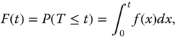
where f(x) is the pdf of T. F(t) gives the probability that the unit fails within time interval (0, t].

2.2.3 Reliability Function

The reliability function (also known as the survival function) of a unit at time t > 0 is defined as

(2.17)

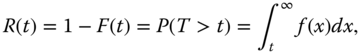
It is the probability that the unit does not fail in time interval (0, t], or the probability that the unit has survived interval (0, t] and is still working at time t.

For the unit with the exponential ttf distribution in Example 2.4, its reliability function at time t is R(t) = e^−λt.

2.2.4 Failure Rate

The failure rate function (also known as hazard rate function) of a unit measures the instantaneous speed of its failure, defined as

2.18

For the unit with the exponential ttf distribution in Example 2.4, its failure rate function is constant, h(t) = λ.

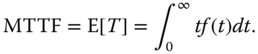
2.2.5 Mean Time to Failure

MTTF is the expected or mean time that a unit will operate before its first failure, which is computed as

(2.19)

Equation (2.20) gives another equivalent formula for computing MTTF:

(2.20)

For the unit with the exponential ttf distribution in Example 2.4, . The probability that the unit will survive its MTTF is R(MTTF) = e⁻¹ = 0.36788.

For a repairable unit, the mean time between failures (MTBF) is typically of interest. It is computed as MTBF = MTTF + MTTR, where MTTR represents the mean time to repair the unit after it is failed. In case of a unit's MTTR being very short or negligible compared to its MTTF, the MTTF can be used to approximate the MTBF of the repairable unit.

2.2.6 Mean Residual Life

The MRL at time (or age) t is the mean remaining lifetime of a unit given that the unit has survived time interval (0, t], which is evaluated as

(2.21)

When the unit is brand new (i.e. age is 0), the MRL at this age is simply MTTF, i.e., MRL(0) = MTTF.

Consider the unit with the exponential ttf distribution in Example 2.4. Because of the memoryless property of the exponential distribution, MRL(t) = MTTF irrespective of the unit's age t, implying that the unit is statistically as good as new as long as the unit is still functioning.

2.3 Fault Tree Modeling

The FT technique was first introduced by Watson at Bell Telephone Laboratories in the 1960s for facilitating an analysis of a launch control system of the Minuteman intercontinental ballistic missile [2]. FT has evolved to be one of the most widely used techniques for system reliability and safety modeling and analysis.

FT is an analytical technique starting with identifying an undesired system event (typically the system considered being in a particular failure mode). Then the system is analyzed to identify all possible combinations of basic component failure events that can cause occurrence of the predefined undesired system event [3]. An FT can graphically represent the logical relationship between the undesired system event and the basic component failure events. It provides a logical framework for comprehending the possible ways in which a system can fail in a certain mode [4].

As a deductive technique, an FT analysis starts with a system failure scenario being considered (corresponding to the TOP event of FT). This failure symptom is then decomposed into its possible causes, each of which is further investigated and decomposed until basic causes of the failure (basic events) are understood. The FT model is completed in levels and constructed from top to bottom. During the top‐down construction process, a set of intermediate events are usually involved. An intermediate event is a fault event that occurs due to one or more antecedent causes acting through logic gates [3] .

There are two types of analysis based on the FT model. A qualitative analysis typically involves identifying minimal cutsets [4] . Each minimal cutset is a minimal combination of basic events whose occurrence results in the occurrence of the TOP event. A quantitative analysis determines the probability of the TOP event (corresponding to system unreliability or unavailability), given the probability of each basic event. Approaches for quantitative FT analysis include simulations (e.g. Monte Carlo simulations) [5] and analytical methods. The analytical methods can be further categorized into three types: state space-based methods [6–9], combinatorial methods [10–12], and modularization methods that integrate the former two methods as appropriate [13,14]. Refer to [15] for a detailed discussion on these methods.

Based on the types of logic gates and events used for constructing the FT model, FT can be classified as static, dynamic, phased‐mission, and multi‐state FTs, which are described in the following sections.

2.3.1 Static Fault Tree

A static fault tree (SFT) represents the system failure criteria in terms of logic AND or OR combinations of fault events. Logical gates used for constructing an SFT are restricted to AND, OR, and VOTE (or K‐out‐of‐N) gates, whose symbols are illustrated in Table 2.2.

Gate	Symbol	Definition
OR		Output event happens if at least one of the gate's input events happens.
AND		Output event happens if all of the gate's input events happen.
VOTE		Output event happens if at least K out of N input events happen.

2.3.2 Dynamic Fault Tree

A dynamic fault tree (DFT) models behavior of a dynamic system through logical gates in Table 2.2 as well as special dynamic gates, such as those illustrated in Table 2.3 [4] .

A cold spare (CSP) gate has one primary basic event, corresponding to the component that is initially powered on and online. It also has one or several alternate basic events, corresponding to standby sparing components that are initially unpowered and serve as replacements for the primary online component. Since a CSP component is fully isolated from operational stresses, its failure rate before being activated can often be assumed as ZERO. The output of a CSP gate occurs when all of its input events have happened, i.e. when the primary component and all the standby sparing components have malfunctioned or become unavailable.

The CSP gate has two variations: hot spare (HSP) gate and warm spare (WSP) gate. Their graphical layouts are similar to that for CSP, with the change of word “CSP” to “HSP” and “WSP,” respectively. An HSP component operates in parallel with the primary online component and is fully exposed to operational stresses; thus, it has the same failure rate before and after being switched into online for use. A WSP component is partially exposed to operational stresses and typically has a reduced failure rate before being switched into active use. Note that a basic event cannot be connected to different types of spare gates within the same system FT model. The reason is that the three spare gates not only model the standby sparing behavior but also affect failure rates of components associated with the gate's input basic events.

A functional dependence (FDEP) gate has a single trigger input event and one or several dependent basic events. The trigger event can be a basic event, or an intermediate event; its occurrence forces the corresponding dependent basic events to happen. An FDEP gate has no logical output; it is typically connected to the top gate of the system FT through a dashed line.

A priority AND (PAND) gate is logically equivalent to the logic AND gate requiring the occurrence of both input events to make the output event happen. However, there is an extra condition that the PAND gate's input events must occur in a predefined order (typically left‐to‐right order in which they appear under the PAND gate). In other words, the output event of a PAND gate will not occur if any of the gate's input events has not occurred or if a right input event occurs before a left input event.

A sequence enforcing (SEQ) gate forces all of the gate's input events to occur in a specified left‐to‐right order. The difference from the PAND gate is the SEQ gate only allows its input events to happen in a predefined order; the PAND gate detects whether its input events take place in the predefined order (these events may occur in any order in practice though).

2.4 Binary Decision Diagram

In 1959, BDDs were first introduced by Lee to represent switching circuits [36]. In 1986, Bryant investigated the full potential for efficient BDD‐based algorithms [37]. Since then, BDD and their extended forms have been applied to diverse application domains [38–48]. In 1993, BDDs were first adapted to the FT reliability analysis of binary‐state systems [ 4 , 10 ,11]. It has been shown by numerous studies that in most cases, the BDD‐based methods require less computational time and memory than other FT reliability analysis methods (e.g. cutsets, pathsets‐based inclusion-exclusion (I‐E) or sum of disjoint products (SDP) methods, and Markov‐based methods). Recently, BDDs and their extended forms have become the state‐of‐the‐art combinatorial models for efficient reliability analysis of diverse types of complex systems. Refer to [49] for a comprehensive discussion of BDD and their extended forms in complex system reliability evaluation.

This section presents basics of BDDs and how to construct and evaluate a BDD model for system reliability analysis.

2.4.1 Basic Concept

BDDs are based on Shannon's decomposition theorem [37] : consider a Boolean expression F on a set of Boolean variables X, thus:

(2.22)

In 2.22, x is a Boolean variable belonging to the set X, F₁ = F_{x = 1} and F₀ = F_{x = 0} represent F evaluated at x being 1 and 0, respectively. To match the notation to the intuitive notion of binary tree induced by the Shannon's decomposition of a Boolean expression, the if‐then‐else (ite) format was introduced [10] .

A BDD is a rooted, directed acyclic graph having two sink nodes and a set of non‐sink nodes. The two sink nodes are labeled by a distinct logic value 0 and 1, representing the system being in a functional or a failed state, respectively. Each non‐sink node is associated with a Boolean variable x, having two outgoing edges called 1‐edge (or then‐edge) and 0‐edge (or else‐edge), respectively (Figure 2.3). The 1‐edge represents the failure of the corresponding component, and it leads to the child node F_x=1; the 0‐edge represents the functioning of the component, and it leads to the child node F_x=0. Each non‐sink node encodes a Boolean function in the ite format (e.g. the non‐sink node in Figure 2.3 encodes 2.22). A key characteristic of the BDD model is that x ⋅ F_{x = 1} and are disjoint.

An ordered binary decision diagram (OBDD) can be obtained by applying the constraint that variables associated with non‐sink nodes are ordered and every path from the root node to the sink node in the BDD model visits the variables in an ascending order. If each non‐sink node in an OBDD encodes a different logic expression, then the OBDD is said to be a reduced ordered binary decision diagram (ROBDD).

ROBDDs can represent logical functions as graphs in a form that is both compact (any other graph representation contains more nodes) and canonical (the representation is unique for a certain variable ordering).

To perform a quantitative reliability analysis of an FT using the ROBDD, the FT is first converted to a ROBDD model (Section 2.4.2), and the resulted ROBDD is then evaluated to generate the system unreliability or reliability (Section 2.4.3).

2.4.2 ROBDD Generation

To construct a ROBDD from an FT, each input variable encoding the binary state of a system component is assigned a different index or order first. The size of the final ROBDD model can heavily rely on the order of these input variables. However, no exact procedure is currently available for determining the optimal ordering of input variables for a given FT structure. Heuristics are typically utilized to find a reasonably good ordering of input variables for ROBDD generation. Refer to [50–55] for several heuristics based on a depth‐first search of the FT model.

After assigning the input variable ordering, OBDD is built in a bottom‐up manner by applying the following operation rules in a recursive manner [37] :

2.23

In 2.23, G and H denote Boolean expressions corresponding to the traversed sub‐FTs. G_i and H_i are subexpressions of G and H, respectively; ⋄ denotes a logic operation (AND or OR).

Specifically, the rules of 2.23 are used to combine two sub‐OBDD models representing logic expressions G and H into one OBDD model. In applying the rules, indexes of the two root nodes (x for G and y for H) are compared. If x and y have the same index (they belong to the same component), then the logic operation is applied to their children nodes (left child node of x with left child node of y, right child node of x with right child node of y); otherwise, the variable having a smaller index becomes the new root node of the combined OBDD model and the logic operation is applied to each child of the node having the smaller index and the other sub‐OBDD as a whole. These rules are recursively applied until one of the sub‐expressions becomes a constant 0 or 1. In this case, the Boolean algebra (1 + x = 1, 0 + x = x, 1 · x = x, 0 · x = 0) is applied to simplify the model.

To generate a ROBDD, two reduction rules are applied: (i) merge isomorphic sub‐OBDDs as one sub‐OBDD because they encode the same Boolean function; and (ii) delete useless nodes, which are nodes with identical left and right child nodes.

2.4.3 ROBDD Evaluation

In the ROBDD generated, each path from the root node to a sink node denotes a disjoint combination of component failures or nonfailures. If the sink node of a path is labeled with 1, then the path leads to the entire system failure; if the sink node of a path is labeled with 0, then the path leads to the entire system function. The probability associated with each else‐edge (or then‐edge) on a path is reliability (or unreliability) of the corresponding component. Because all the paths in a ROBDD are disjoint, the system unreliability (reliability) can be simply evaluated by adding probabilities of all the paths from the root node to sink node 1 (0).

The recursive evaluation algorithm in the computer implementation with regard to the OBDD branch in Figure 2.3 can be represented as:

where q_x and p_x represent the unreliability and reliability of component x. P(F) gives the final system unreliability when x is the root node of the entire system ROBDD. The exit condition of this recursive algorithm is: If F = 0, then P(F) = 0; If F = 1, then P(F) = 1.

2.5 Markov Process

As discussed in Section 2.3, the state space‐based methods belong to the analytical methods for system reliability analysis. Among the state space‐based methods, Markov models particularly, continuous‐time Markov chains (CTMCs) have commonly been applied to analyze reliability of systems with dynamic behavior and exponential component ttf distributions [7, 15 ].

Constructing a Markov model involves identifying system states and possible transitions among these states. In the Markov‐based system reliability analysis, each state typically denotes a distinct combination of failed and functioning components. A state transition governs the change of the system from one state to another state due to events such as failure of a component or repair of a component. Each state transition is characterized by certain parameter(s), such as a component's failure rate or repair rate [56]. The state transition diagram starts with an initial state (typically a state in which all the system components are fault free). As time passes and component failures take place, the system goes from one state to another until one of the system failure states is reached.

Based on the state transition diagram generated, a set of differential equations AP(t) = P′(t) is constructed with A representing the state transition rate matrix, P(t) representing the vector of the system state probability at time t, and P′(t) representing the vector of the derivative of the system state probability at time t. Equation (2.26) shows the detailed form of the state equations for a system with n states.

(2.26)

In 2.26, P_j(t) denotes the probability of the system being in state j at time t, j = 1, 2, …, n. α_jk(j ≠ k) denotes the transition rate from state j to state k. The diagonal element is obtained as (the sum of departure rates from state j). Hence, the sum of each column of the matrix A is zero.

2.6 Reliability Software

Various reliability analysis software tools have been developed. For example, Galileo, originally developed at the University of Virginia, is a reliability analysis tool based on the DFT analysis methodology [61]. This software tool implements the modular approach (described in Section 2.5 ), where diverse time‐to‐failure distributions (e.g. exponential, Weibull, lognormal) and fixed failure probabilities are supported in the BDD‐based solution to static sub‐FTs. Galileo supports reliability analysis of PMSs.

Another FT‐based reliability analysis software package is Isograph's FaultTree+ [62]. This software includes three modules, respectively, supporting FT analysis, event tree analysis, and Markov analysis. FaultTree+ has recently been incorporated into Reliability Workbench, the Isograph's flagship suite of reliability software.

ReliaSoft BlockSim [63] is a comprehensive software developed for reliability, availability, maintainability, and related analyses of both repairable and nonrepairable systems. This software supports modeling using FTs and reliability block diagrams. It also supports modeling some complex configurations such as standby redundancy, load sharing, and phased‐missions.

References

1. 1 Allen, A. (1990). Probability, Statistics and Queuing Theory: with Computer Science Applications, 2e. Academic Press.
2. 2 Watson, H.A. (1961). Launch Control Safety Study. Murray Hill, NJ: Bell Telephone Laboratories.
3. 3 Vesely, W.E., Goldberg, F.F., Roberts, N.H., and Haasl, D.F. (1981). Fault Tree Handbook. Washington, DC: U.S. Nuclear Regulatory Commission.
4. 4 Dugan, J.B. and Doyle, S.A. (1996). New results in fault‐tree analysis. In: Tutorial Notes of Annual Reliability and Maintainability Symposium, Las Vegas, NV, USA.
5. 5 Ke, J., Su, Z., Wang, K., and Hsu, Y. (2010). Simulation inferences for an availability system with general repair distribution and imperfect fault coverage. Simulation Modelling Practice and Theory 18 (3): 338–347.
6. 6 Bobbio, A., Franceschinis, G., Gaeta, R., and Portinale, L. (1999). Exploiting petri nets to support fault tree based dependability analysis. In: Proceedings of the 8th International Workshop on Petri Nets and Performance Models, 146–155.
7. 7 Dugan, J.B., Bavuso, S.J., and Boyd, M.A. (1993). Fault trees and Markov models for reliability analysis of fault tolerant systems. Reliability Engineering & System Safety 39: 291–307.
8. 8 Hura, G.S. and Atwood, J.W. (1988). The use of petri nets to analyze coherent fault trees. IEEE Transactions on Reliability 37 (5): 469–474.
9. 9 Malhotra, M. and Trivedi, K.S. (1995). Dependability modeling using petri nets. IEEE Transactions on Reliability 44 (3): 428–440.
10. 10 Rauzy, A. (1993). New algorithms for fault tree analysis. Reliability Engineering & System Safety 40: 203–211.
11. 11 Coudert, O. and Madre, J.C. (1993). Fault tree analysis: 10²⁰ prime implicants and beyond. In: Proceedings of Annual Reliability and Maintainability Symposium. Atlanta, GA, USA.
12. 12 Sinnamon, R. and Andrews, J.D. (1996). Fault tree analysis and binary decision diagrams. In: Proceedings of the Annual Reliability and Maintainability Symposium. Las Vegas, NV, USA.
13. 13 Gulati, R. and Dugan, J.B. (1997). A modular approach for analyzing static and dynamic fault trees. In: Proceedings of the Annual Reliability and Maintainability Symposium. Philadelphia, PA, USA.
14. 14 Sahner, R., Trivedi, K.S., and Puliafito, A. (1996). Performance and Reliability Analysis of Computer Systems: An Example‐Based Approach Using the SHARPE Software Package. Kluwer Academic Publisher.
15. 15 Xing, L. and Amari, S.V. (2008). Fault tree analysis. In: Handbook of Performability Engineering. Springer‐Verlag.
16. 16 Xing, L. (2007). Reliability importance analysis of generalized phased‐mission systems. International Journal of Performability Engineering 3 (3): 303–318.
17. 17 Astapenko, D. and Bartlett, L.M. (2009). Phased mission system design optimisation using genetic algorithms. International Journal of Performability Engineering 5 (4): 313–324.
18. 18 Dai, Y., Levitin, G., and Xing, L. (2014). Structure optimization of non‐repairable phased mission systems. IEEE Transactions on Systems, Man, and Cybernetics: Systems 44 (1): 121–129.
19. 19 Alam, M., Min, S., Hester, S.L., and Seliga, T.A. (2006). Reliability analysis of phased-mission systems: a practical approach. In: Proceedings of Annual Reliability and Maintainability Symposium. Newport Beach, CA. USA.
20. 20 Murphy, K.E., Carter, C.M., and Malerich, A.W. (2007). Reliability analysis of phased‐mission systems: a correct approach. In: Proceedings of Annual Reliability and Maintainability Symposium. Orlando, FL.
21. 21 Dugan, J.B. (1991). Automated analysis of phased‐mission reliability. IEEE Transactions on Reliability 40 (1): 45–52,55.
22. 22 Smotherman, M.K. and Zemoudeh, K. (1989). A non‐homogeneous Markov model for phased‐mission reliability analysis. IEEE Transactions on Reliability 38 (5): 585–590.
23. 23 Mura, I. and Bondavalli, A. (2001). Markov regenerative stochastic petri nets to model and evaluate phased mission systems dependability. IEEE Transactions on Computers 50 (12): 1337–1351.
24. 24 Esary, J.D. and Ziehms, H. (1975). Reliability analysis of phased missions. In: Reliability and fault tree analysis: theoretical and applied aspects of system reliability and safety assessment, 213–236. Philadelphia, PA: SIAM.
25. 25 Somani, A.K. and Trivedi, K.S. (1997). Boolean algebraic methods for phased‐mission system analysis. Technical Report NAS1–19480. NASA Langley Research Center, Hampton, Virginia, USA.
26. 26 Xing, L. and Dugan, J.B. (2002). Analysis of generalized phased mission system reliability, performance and sensitivity. IEEE Transactions on Reliability 51 (2): 199–211.
27. 27 Xing, L. and Levitin, G. (2011). Combinatorial algorithm for reliability analysis of multi‐state systems with propagated failures and failure isolation effect. IEEE Transactions on Systems, Man, and Cybernetics, Part A: Systems and Humans 41 (6): 1156–1165.
28. 28 Shrestha, A., Xing, L., and Dai, Y.S. (2011). Reliability analysis of multi‐state phased‐mission systems with unordered and ordered states. IEEE Transactions on Systems, Man, and Cybernetics, Part A: Systems and Humans 41 (4): 625–636.
29. 29 Levitin, G. and Xing, L. (2010). Reliability and performance of multi‐state systems with propagated failures having selective effect. Reliability Engineering & System Safety 95 (6): 655–661.
30. 30 Huang, J. and Zuo, M.J. (2004). Dominant multi‐state systems. IEEE Transactions on Reliability 53 (3): 362–368.
31. 31 Levitin, G. (2003). Reliability of multi‐state systems with two failure‐modes. IEEE Transactions on Reliability 52 (3): 340–348.
32. 32 Chang, Y.‐R., Amari, S.V., and Kuo, S.‐Y. (2005). OBDD‐based evaluation of reliability and importance measures for multistate systems subject to imperfect fault coverage. IEEE Transactions on Dependable and Secure Computing 2 (4): 336–347.
33. 33 Li, W. and Pham, H. (2005). Reliability modeling of multi‐state degraded systems with multi‐competing failures and random shocks. IEEE Transactions on Reliability 54: 297–303.
34. 34 Zang, X., Wang, D., Sun, H., and Trivedi, K.S. (2003). A BDD‐based algorithm for analysis of multistate systems with multistate components. IEEE Transactions on Computers 52 (12): 1608–1618.
35. 35 Amari, S.V., Xing, L., Shrestha, A. et al. (2010). Performability analysis of multi‐state computing systems using multi‐valued decision diagrams. IEEE Transactions on Computers 59 (10): 1419–1433.
36. 36 Lee, C.Y. (1959). Representation of switching circuits by binary‐decision programs. Bell Systems Technical Journal 38: 985–999.
37. 37 Bryant, R.E. (1986). Graph‐based algorithms for Boolean function manipulation. IEEE Transactions on Computers 35 (8): 677–691.
38. 38 Miller, D.M. (1993). Multiple‐valued logic design tools. In: Proceedings of 23rd International Symposium on Multiple‐Valued Logic (ISMVL), 2–11. Sacramento, CA, USA.
39. 39 Miller, D.M. and Drechsler, R. (1998). Implementing a multiple‐valued decision diagram package. In: Proceedings of 23rd International Symposium on Multiple‐Valued Logic (ISMVL), 52–57. Fukuoka, Japan.
40. 40 Burch, J.R., Clarke, E.M., Long, D.E. et al. (1994). Symbolic model checking for sequential circuit verification. IEEE Transactions on Computer‐Aided Design of Integrated Circuits and Systems 13 (4): 401–424.
41. 41 Ciardo, G. and Siminiceanu, R. (2001). Saturation: an efficient iteration strategy for symbolic state space generation. In: Tools and Algorithms for the Construction and Analysis of Systems, 328–342.
42. 42 Hermanns, H., Meyer‐Kayser, J., and Siegle, M. (1999). Multi terminal binary decision diagrams to represent and analyse continuous time Markov chains. In: Numerical Solution of Markov Chains, 188–207.
43. 43 Miner, A.S. and Cheng, S. (2004). Improving efficiency of implicit Markov chain state classification. In: Proceedings of First International Conference on the Quantitative Evaluation of Systems (QEST ‘04), 262–271. Enschede, The Netherlands.
44. 44 Ciardo, G. (2004). Reachability set generation for petri nets: can brute force be smart. In: Proceedings of 25th International Conference on the Applications and Theory of Petri Nets (ICATPN ‘04), 17–34.
45. 45 Miner, A.S. and Ciardo, G. (1999). Efficient reachability set generation and storage using decision diagrams. In: Application and Theory of Petri Nets, 6–25.
46. 46 Burch, J.R., Clarke, E.M., McMillan, K.L. et al. (1990). Symbolic model checking: 10²⁰ states and beyond. In: Proceedings of Fifth Annual IEEE Symposium on the Logic in Computer Science (LICS' 90), 1–33. Philadelphia, PA, USA.
47. 47 Chechik, M., Gurfinkel, A., Devereux, B. et al. (2006). Data structures for symbolic multi‐valued model‐checking. Formal Methods in System Design 29 (3): 295–344.
48. 48 Corsini, M.‐M. and Rauzy, A. (1994). Symbolic model checking and constraint logic programming: a cross‐fertilization. In: Proceedings of Fifth European Symp. Programming (ESOP'94), 180–194.
49. 49 Xing, L. and Amari, S.V. (2015). Binary Decision Diagrams and Extensions for System Reliability Analysis. Salem, MA: Wiley‐Scrivener.
50. 50 Minato, S., Ishiura, N., and Yajima, S. (1990). Shared binary decision diagrams with attributed edges for efficient Boolean function manipulation. In: Proceedings of the 27th ACM/IEEE Design Automation Conference, 52–57. Orlando, FL, USA.
51. 51 Fujita, M., Fujisawa, H., and Kawato, N. (1988). Evaluation and improvements of Boolean comparison method based on binary decision diagrams. In: Proceedings of IEEE International Conference on Computer Aided Design, 2–5. Santa Clara, CA, USA.
52. 52 Fujita, M., Fujisawa, H., and Matsugana, Y. (1993). Variable ordering algorithm for ordered binary decision diagrams and their evaluation. IEEE Transactions on Computer‐Aided Design of Integrated Circuits and Systems 12 (1): 6–12.
53. 53 Bouissou, M., Bruyere, F., and Rauzy, A. (1997). BDD based fault‐tree processing: a comparison of variable ordering heuristics. In: Proceedings of ESREL Conference, Lisbon, Portugal.
54. 54 Bouissou, M. (1996). An ordering heuristics for building binary decision diagrams from fault‐trees. In: Proceedings of the Annual Reliability and Maintainability Symposium. Las Vegas, NV, USA.
55. 55 Butler, K.M., Ross, D.E., Kapur, R., and Mercer, M.R. (1991). Heuristics to compute variable orderings for efficient manipulation of ordered BDDs. In: Proceedings of the 28th Design Automation Conference. San Francisco, CA, USA.
56. 56 Gulati, R. (1996). A modular approach to static and dynamic fault tree analysis. M. S. Thesis, Electrical Engineering, University of Virginia.
57. 57 Sune, V. and Carrasco, J.A. (1997). A method for the computation of reliability bounds for non‐repairable fault‐tolerant systems. In: Proceedings of the 5th IEEE International Symposium on Modeling, Analysis, and Simulation of Computers and Telecommunication System, 221–228. Haifa, Israel.
58. 58 Sune, V. and Carrasco, J.A. (2001). A failure‐distance based method to bound the reliability of non‐repairable fault‐tolerant systems without the knowledge of minimal cutsets. IEEE Transactions on Reliability 50 (1): 60–74.
59. 59 Manian, R., Dugan, J.B., Coppit, D., and Sullivan, K.J. (1998). Combining various solution techniques for dynamic fault tree analysis of computer systems. In: Proceedings of the 3rd IEEE International High‐Assurance Systems Engineering Symposium, 21–28. Washington, DC, USA.
60. 60 Dutuit, Y. and Rauzy, A. (1996). A linear time algorithm to find modules of fault trees. IEEE Transactions on Reliability 45 (3): 422–425.
61. 61 Sullivan, K.J., Dugan, J.B., and Coppit, D. (1999). The Galileo fault tree analysis tool. In: Proceedings of the 29th International Symposium on Fault‐Tolerant Computing. Madison, WI, USA.
62. 62 FaultTree+, https://www.isograph.com/software/reliability‐workbench/fault‐tree‐analysis‐software, accessed in March 2018.
63. 63 BlockSim, https://www.reliasoft.com/products/reliability‐analysis/blocksim, accessed in March 2018.