
8
Deterministic Competing Failure
8.1 Overview
A propagated failure with global effect (PFGE) that originates from a system component causes the failure of the entire system [1]. As one type of common‐cause failures (CCFs), PFGEs have been investigated intensively in literature (see, e.g. [2–6]). Examples of causes for PFGEs include imperfect coverage (IPC) and destructive effects. Specifically, as discussed in Chapter 3, due to the IPC, a component fault, if not being detected or located successfully by the system recovery mechanism, may propagate and cause an overall system failure even when adequate redundancy remains. Certain types of failures originating from a system component can cause destructive effects on other components, for example, fire, explosion, overheating, blackout, or short circuit may incapacitate or destroy all other system components, causing the failure of the entire system.
However, it is not necessarily always the truth that a PFGE causes the entire system failure, particularly for systems undergoing the Functional DEPendence (FDEP) behavior. As described in Chapter 5 , with the FDEP, a trigger event, upon occurring, can isolate the corresponding dependent components (making them unusable or inaccessible) deterministically. Due to this isolation effect, a PFGE originating from a dependent component can thus be isolated without affecting other portions of the system. For example, in a clustered wireless sensor network (WSN) system, sensor nodes within a cluster are accessed through their cluster head [7]. In other words, these sensor nodes have FDEP on the cluster head. If the cluster head fails, PFGEs originating from any of the sensor nodes within the cluster can be isolated from the rest of the WSN system. Note that the failure isolation effect can take place only when the trigger event occurs before the occurrence of any PFGE originating from the corresponding dependent components. On the other hand, if any PFGE from a dependent component occurs before the trigger event happens, the global failure propagation effect takes place causing an entire system failure.
In summary, competitions exist in the time domain between the failure isolation effect and the failure propagation effect; different occurrence sequences lead to different system statuses. In this chapter, a separable method for handling PFGEs in system reliability analysis is first discussed. Based on this approach, methods are then presented for addressing the competing effects in the reliability analysis of different types of nonrepairable systems, including single‐phase system with single FDEP group, single‐phase system with multiple dependent FDEP groups, single‐phase system subject to propagated failures (PFs) with global and selective effects, multi‐phase system (or phased‐mission system, PMS) with single FDEP group, and PMS with multiple independent or dependent FDEP groups.
8.2 PFGE Method
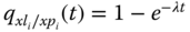
Til and Tip are random variables respectively representing the time‐to‐local‐failure and the time‐to‐PFGE of a system component i. fil(t) and fip(t) represent the probability density function (pdf) of Til and Tip, respectively. qil(t) and qip(t) are unconditional local and propagated failure probabilities of component i at time t, respectively. Thus, ![]() and
and ![]() .
.
According to the simple and efficient algorithm (SEA) in Section 3.3.2 [ 2 ,4], the system unreliability can be evaluated based on the total probability law as:
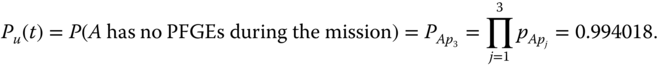
with Pu(t) being defined and computed as
Q(t) in 8.1 is defined as a conditional system failure probability given that no PFGEs take place during the considered mission time. The evaluation of Q(t) requires no consideration of effects from PFGEs and thus can be performed using any approaches ignoring PFGEs, e.g. the binary decision diagram (BDD)–based methods [ 4 , 7 ] for single‐phase systems (Section 2.4) and PMSs (Section 3.5.3).
As in the SEA method, the evaluation of Q(t) requires the calculation of a conditional component failure probability qi(t) given that no PFGEs occur to the component. The evaluation method is illustrated for different statistical relationships between the local failure (LF) and PFGE in the following sections.
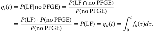
8.2.1 s‐Independent LF and PFGE
When the LF and PFGE of the same component are s‐independent, the conditional component failure probability is evaluated as
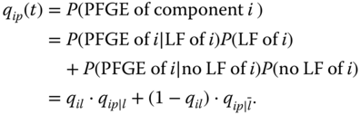
8.2.2 s‐Dependent LF and PFGE
When the LF and PFGE of the same component are s‐dependent, the conditional component failure probability is evaluated as
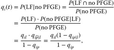
where,
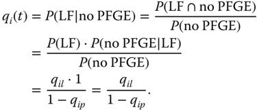
8.2.3 Disjoint LF and PFGE
When the LF and PFGE of the same component are disjoint or mutually exclusive, the conditional component failure probability is evaluated as
8.3 Single‐Phase System with Single FDEP Group
Based on the PFGE method, a combinatorial methodology is discussed in this section for analyzing reliability of a single‐phase system subject to competing failures involved in a single FDEP group or multiple independent (nonoverlapped) FDEP groups. The method is applicable to any arbitrary ttf distributions for the system components.
8.3.1 Combinatorial Method
Given that the trigger component(s) can only experience LFs. The method contains the following three steps:
- Step 1: Define FDEP‐related events and evaluate event occurrence probabilities. Three events representing different occurrence sequences of the trigger event and PFGE events of the corresponding dependent components are defined as follows:
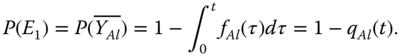
- E1: the trigger event does not take place (i.e. the trigger component does not fail locally). Assume that the unconditional LF event of trigger component, e.g. A is YAl. P(E1) is calculated as:
(8.7)
Note that in the case of the trigger component being subject to PFGEs in addition to the LF, the PFGE method presented in Section 8.2 should be applied to separate the global failure propagation effect originating from the trigger component before Step 1. qAl(t) in 8.7 should be, respectively, replaced with qA(t) evaluated using 8.3, 8.4, or 8.6 when the LF and PFGE of the trigger component are independent, dependent, or disjoint. Accordingly, the pdf of time‐to‐LF of trigger component A involved in 8.11, i.e. fAl(τ2) should be evaluated as dqA(t)/dt.
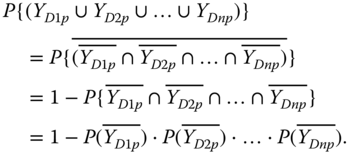
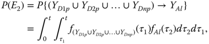
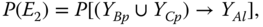
- E2: at least one PFGE of dependent components takes place before the trigger LF event occurs. Assume the trigger component A affects n dependent components D1, D2, ..., Dn, i.e. the fuctional dependence group (FDG) for component A is FDGA = {D1, D2, ..., Dn}. The PFGE events of these dependent components are represented by YD1p, YD2p, ... , and YDnp and are s‐independent. Thus, P(E2) is evaluated as:
- E1: the trigger event does not take place (i.e. the trigger component does not fail locally). Assume that the unconditional LF event of trigger component, e.g. A is YAl. P(E1) is calculated as:
where
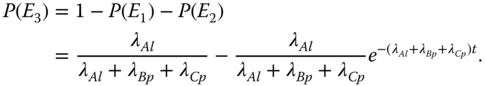
In general, for n components with their ttf r.v.s represented by X1, …, Xn, the probability of their sequential failures is evaluated as [8]:

Thus, 8.8 can be evaluated as
where

By definition, in the case of the dependent components undergoing no PFGEs, P(E2) = 0.
- E3: the trigger event takes place before the occurrence of any PFGE originating from the dependent components. Under this event, the failure isolation effect takes place. Since E1, E2, and E3 form a complete event space, one obtain
(8.13)

- Step 2: Evaluate P(system fails|Ei) for i∈{1, 2, 3}.
- P(system fails|E1): based on the system fault tree (FT) after removing the FDEP gate and its trigger component(s), P(system fails|E1) is evaluated by applying the PFGE method described in Section 8.2 .
- P(system fails|E2): because when at least one PFGE takes place, the entire system fails due to the global failure propagation effect, P(system fails|E2) = 1.
- P(system fails|E3): a reduced FT that considers the failure isolation effect is generated. Firstly, the FDEP gate and its trigger component(s) are removed from the original system FT. Failure events of the corresponding dependent components are then replaced with constant 1 (TURE). Boolean algebra rules (1 + x = 1 and 1 · x = x, where x represents a Boolean variable) are finally applied to generate the reduced FT. Based on the reduced FT, if any component appearing in the reduced FT undergoes PFGEs, the PFGE method described in Section 8.2 is applied to evaluate P(system fails|E3); otherwise, any traditional approach ignoring PFGEs, e.g. the BDD‐based method is applied to solve P(system fails|E3).
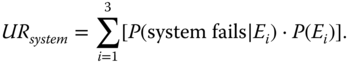
- Step 3: Integrate for final system unreliability. Based on the total probability law [9], the system unreliability is evaluated by integrating P(Ei) and P(system fails|Ei) as [10]:
(8.14)
8.3.2 Case Study
The LF probability and the PFGE probability are, respectively:

When the LF and PFGE of component B or C are s‐dependent, conditional PGFE failure rates conditioned on occurrence or nonoccurrence of an LF (λBp | l, ![]() , λCp | l,
, λCp | l, ![]() ) are given. Two types of dependencies can be modeled [11]: positive dependence takes place if the LF of a component causes an increased tendency of the component's PFGE (thus, e.g. λBp | l>
) are given. Two types of dependencies can be modeled [11]: positive dependence takes place if the LF of a component causes an increased tendency of the component's PFGE (thus, e.g. λBp | l>![]() ); negative dependence takes place if the LF of a component causes a reduced tendency of the component's PFGE (thus, e.g. λBp | l <
); negative dependence takes place if the LF of a component causes a reduced tendency of the component's PFGE (thus, e.g. λBp | l < ![]() ).
).
Input Parameters. The following values are used in the illustrative analysis: λAl = 0.0001/hr, λBl = λCl = λDl = 0.0002/hr. For component B or C, two sets of parameters are considered. If the LF and PFGE are s‐independent or disjoint, λBp = λCp = 0.00001/hr; if the LF and PFGE are s‐dependent, λBp | l=λCp | l=0.00003/hr and ![]() /hr (positive dependence).
/hr (positive dependence).
Example Analysis. The s‐independent case is used to illustrate the combinatorial method in detail.
- Step 1: Define FDEP‐related events and evaluate their occurrence probabilities, as follows:
- E1: trigger component A does not fail (locally). According to 8.7 and 8.16,
(8.17)

- E2: at least one PFGE from B and C takes place before the trigger event occurs. According to 8.8,
(8.18)where, according to 8.9,
 8.19
8.19
Further, based on 8.12,
(8.20) 8.21
8.21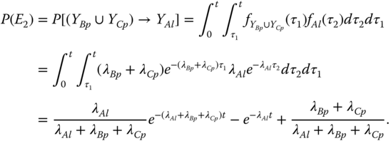
- E3: the LF of trigger component A takes place before any PFGE originating from the dependent components happens. According to 8.13,
8.22
- E1: trigger component A does not fail (locally). According to 8.7 and 8.16,
- Step 2: Evaluate P(system fails|Ei) for i∈{1, 2, 3}.
P(system fails|E1): under E1, no failure isolation effect takes place. Figure 8.3 shows the FT after removing the FDEP gate and its trigger component A. Based on the FT in Figure 8.3 , P(system fails|E1) is evaluated using the PFGE method (Section 8.2 ) as follows.
According to 8.1,
(8.23)
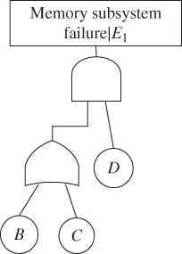
Figure 8.3 Reduced FT for P(system fails|E1).
where, based on 8.2,
(8.24)
To evaluate Q(t) in 8.23, component conditional failure probabilities are computed. For the s‐independent case, 8.3 is adopted for the computation, that is,
8.25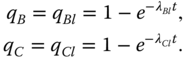
Figure 8.4 shows the BDD model generated from the FT in Figure 8.3 for Q(t) in 8.23.
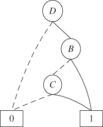
Figure 8.4 BDD model for evaluating Q(t).
Evaluating the BDD of Figure 8.4 using the component conditional failure probabilities computed using 8.25, Q(t) is obtained as
8.26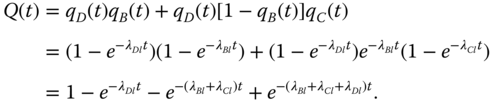
Based on 8.23, 8.24, and 8.26 are integrated to obtain 8.27.
8.27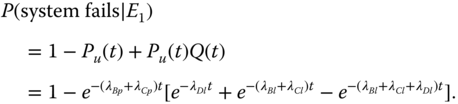
Under E2, since the global failure propagation effect takes place. Therefore,
(8.28)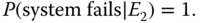
Under E3, the failure isolation effect takes place. Figure 8.5 shows the reduced FT generated for evaluating P(system fails|E3). Thus,
(8.29)
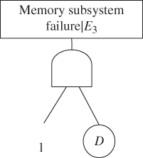
Figure 8.5 Reduced FT for P(system fails|E3).
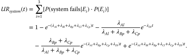
- Step 3: Integrate for final system unreliability. Based on 8.14, the unreliability of the example memory subsystem is obtained as
8.30
In the case of LF and PFGE of component B or C being s‐dependent or disjoint, the combinatorial method presented in Section 8.3.1 can be similarly applied to derive the system unreliability.
Using the given parameter values, the unreliability of the example memory subsystem under the three cases is summarized in Table 8.1. The system unreliability in the s‐independent case is lower than that in the disjoint case. This is because that for the same component parameter values, the component reliability in the s‐independent case (calculated as [1 − qil(t)]·[1 − qip(t)]) is higher than that in the disjoint case (calculated as 1 − qil(t) − qip(t)). The system unreliability in the s‐dependent case is higher than that in the s‐independent or disjoint case due to the positive dependence assumed in the example input parameters.
Table 8.1 Unreliability of the example memory sub‐system.
| Mission time t (hrs) | 1000 | 5000 | 10 000 |
| s‐dependent | 0.0943 | 0.6417 | 0.8949 |
| s‐independent | 0.0889 | 0.6128 | 0.8757 |
| disjoint | 0.0894 | 0.6207 | 0.8799 |
8.4 Single‐Phase System with Multiple FDEP Groups
This section considers the reliability analysis of a single‐phase system subject to competing failures involved in multiple dependent FDEP groups. The method is applicable to any arbitrary ttf distributions for the system components.
8.4.1 Combinatorial Method
The combinatorial method contains the following three steps [12]:
- Step 1: Construct an event space based on statuses of trigger components. Given m trigger components (denoted by Ti, i = 1 ,…, m) involved in FDEPs, an event space consists of 2m events, each called a combined trigger event (CTE), and is constructed as follows:
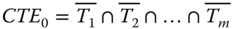 ,
, 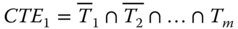 , ……,
, ……,  . Based on the total probability law [9]
, the system unreliability is evaluated as
(8.31)
. Based on the total probability law [9]
, the system unreliability is evaluated as
(8.31)
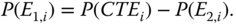
- Step 2: Evaluate P(system failure|CTEi)P(CTEi). Each CTEi is decomposed into two complementary events defined as follows:
- E1,i: all PFGEs either do not occur or are isolated by failures of corresponding trigger components.
- E2,i: at least one PFGE is not isolated. It takes place when any PFGE occurs to a dependent component in the FDEP group where the corresponding trigger component does not fail or fails after the PFGE. As evaluating P(E2,i) is more straightforward than evaluating P(E1,i), P(E2,i) is computed first, P(E1,i) is then evaluated as
(8.32)
P(system failure|CTEi)P(CTEi) can be evaluated as
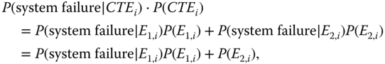
where P(system failure|E2,i) = 1 due to the global failure propagation effect.
Under E1,i, all PFGEs from dependent components either do not happen or are isolated. A reduced FT is generated for evaluating P(system failure|E1,i) in 8.33. Under each considered CTEi, the trigger event and corresponding FEDP gate are first removed from the original system FT. If a trigger event occurs, then events of the corresponding dependent components are replaced with constant 1 (TRUE); otherwise, events of the dependent components remain in the FT. Boolean algebra rules are then applied to simplify the FT. The reduced FT generated can be evaluated using the BDD method [13] to find P(system failure|E1,i).
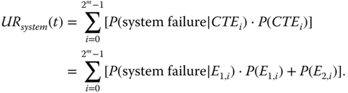
- Step 3: Integrate for final system unreliability. Based on 8.31 and 8.33, results of step 2 are integrated to obtain the system unreliability, considering competing failures involved in multiple FDEP groups.
8.34
Note that the above three‐step procedure does not address PFGEs from nondependent components. In the case of nondependent components undergoing PFGEs, a pre‐processing step 0 described below is applied based on the PFGE method (Section 8.2 ):
- Step 0: Separate PFGEs of all nondependent components from the solution combinatorics. Based on the PFGE method, the system unreliability is evaluated as 8.1, where Pu(t) represents the probability that no PFGEs from nondependent components (including trigger components) occur. Q(t) in 8.1 is defined as the conditional system failure probability given that no PFGEs from nondependent components occur, which is evaluated using the above described three‐step procedure.
8.4.2 Case Study

Figure 8.6 FT of the example memory system.
Input Parameters. The exponential distribution is assumed for this illustrative example. The pdf and cdf of the exponential distribution with failure rate λ are given in 8.35.
The three MCs undergo both LFs and PFGEs with constant rates given in Table 8.2. The LF and PFGE of the same MC are s‐independent. The two MIUs only experience LFs with rates also given in Table 8.2 .
Table 8.2 Failure rates of the example memory system components (/hr).
| Component | PFGE rate | LF rate |
| MCi | 0.00005 | 0.0002 |
| MIUi | 0 | 0.0001 |
Example Analysis. The unreliability of the example memory system at time t = 1000 hours is analyzed using the method of Section 8.4.1 as follows.
- Step 1: Construct an event space based on statuses of trigger components. The two trigger components lead to an event space with 4 CTEs defined in 8.36.


 (8.36)
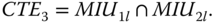
- Step 2: Evaluate P(system failure|CTEi)P(CTEi)
- Evaluate P(system failure|CTE0)P(CTE0). Under CTE0, no trigger components fail. Thus,
(8.37)

Under CTE0, if any PFGE from a dependent component occurs, E2,0 takes place. So,
8.38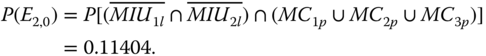
Thus,
(8.39)
Figure 8.7 shows the reduced FT for evaluating P(system failure | E1,0). Figure 8.8 shows the BDD model generated from the FT. The evaluation of the BDD model in Figure 8.8 gives
8.40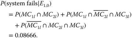
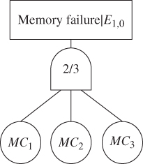
Figure 8.7 Reduced FT for P(system failure | E1,0).

Figure 8.8 BDD for P(system failure | E1,0).
- Evaluate P(system failure|CTE1)P(CTE1).
Under CTE1, only MIU2 fails locally. Thus,

Under CTE1, if any PFGE from MC1 or MC2 happens, or PFGE from MC3 happens before MIU2 fails, then event E2,1 takes place. So

The evaluation of P(E2,1) involves an sequential event, which can be evaluated using 8.10. With P(E2,1), one obtain P(E1,1) = P(CTE1) − P(E2,1) = 0.07603.
Figure 8.9 shows the reduced FT for evaluating P(system failure | E1,1). Figure 8.10 shows the BDD model generated from the FT. The evaluation of the BDD model in Figure 8.10 gives P(system failure | E1,1) = 0.32968.
- Evaluate P(system failure|CTE2)P(CTE2).
Under CTE2, only MIU1 fails locally. Thus,

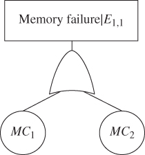
Figure 8.9 Reduced FT for P(system failure | E1,1).

Figure 8.10 BDD for P(system failure | E1,1).
Under CTE2, if any PFGE from MC2 or MC3 happens, or PFGE from MC1 happens before MIU1 fails, then event E2,2 takes place. So,

Thus, P(E1,2) = P(CTE2) − P(E2,2) = 0.07603.
Figure 8.11 shows the reduced FT for evaluating P(system failure | E1,2). Figure 8.12 shows the BDD model generated from the FT. The evaluation of the BDD model in Figure 8.12 gives P(system failure | E1,2) = 0.32968.
- Evaluate P(system failure|CTE3)P(CTE3).
Under CTE3, both trigger components fail. Thus,

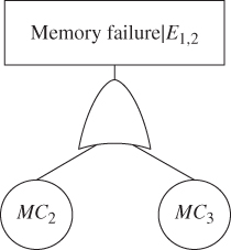
Figure 8.11 Reduced FT for P(system failure | E1,2).
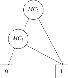
Figure 8.12 BDD for evaluating P(system failure | E1,2).
Under CTE3, if at least one PFGE from the three MCs happens before the corresponding trigger component fails, then event E2,3 takes place. So,
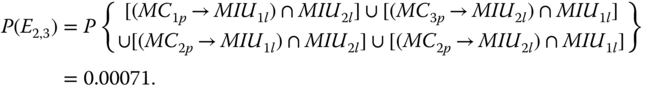
Thus,

When both of the trigger components fail, the entire system fails. Therefore P(system failure | E1,3) = 1.
- Evaluate P(system failure|CTE0)P(CTE0). Under CTE0, no trigger components fail. Thus,
- Step 3: Integrate for final system unreliability. According to 8.34, results obtained at step 2 are integrated to obtain the final system unreliability as

8.5 Single‐Phase System with PFs Having Global and Selective Effects
A PF that originates from a system component causes extensive damages to the rest of the system. A PFGE occurs when the PF causes the entire system to fail. There also exist a propagated failure with selective effect (PFSE), which takes place when the PF causes failure of only a subset of system components. This section presents a combinatorial reliability analysis method for single‐phase systems subject to competing failures considering both global and selective propagation effects [14].
8.5.1 Combinatorial Method
The combinatorial reliability analysis method can be described as a seven‐step procedure:
- Step 1: Define events representing states of the trigger component. Two disjoint events are defined:
- E1: the trigger component is functioning correctly.
- E2: the trigger component is failed.
Based on the total probability law, the system unreliability is evaluated as
(8.41)
- Step 2: Evaluate occurrence probability of E1. P(E1) in 8.41 is simply the reliability of the trigger component.
- Step 3: Evaluate P(system fails|E1). Given that E1 happens, no failure isolation effect takes place. The PFGE method (Section 8.2
) is applied to evaluate P(system fails | E1) as
(8.42)

where Pu(t) = P(no PFGEs) and Q(t) = P(system fails|no PFGEs). While the PFGEs are separated from the solution combinatorics via the PFGE method, the PFSEs have to be addressed in the evaluation of Q(t) as follows.
Given that up to m independent PFSEs may occur when the trigger component functions, an event space with 2m events (denoted by SEi) is constructed, each being a combination of occurrence or nonoccurrence of these m PFSEs. Based on the total probability law, Q(t) in 8.42 is computed as
(8.43)
where P(system fails |SEi) can be obtained through the BDD‐based evaluation of a reduced FT. The reduced FT is generated by the following procedure:
- Remove the FDEP gate and its trigger component from the original system FT.
- Replace events of components affected by SEi with constant 1.
- Apply Boolean algebra rules to simplify the FT.
- Step 4: Define two disjoint event cases given that E2 takes place. Given that E2 happens (i.e. the trigger component fails), two disjoint cases are considered for evaluating P(system fails|E2) P(E2) in 8.41:
- Case a: At least one PFGE from any dependent components occurs before E2 happens. Under this case, the global failure propagation effect destroys the entire system, i.e. P(system fails|Case a) =1.
- Case b: No PFGEs occur before E2 happens.
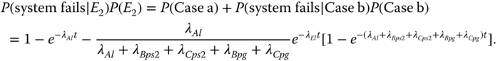
Based on the total probability law, P(system fails|E2)P(E2) is calculated as
8.44
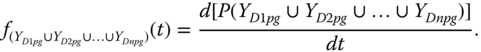
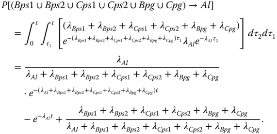
- Step 5: Evaluate P(Case a). Assume that the trigger component A has n dependent components D1, D2, ... Dn, whose PFGE events are denoted as YD1pg, YD2pg, ...,YDnpg, respectively. Thus, P(Case a) = P[(YD1pg ∪ YD2pg ∪ … ∪ YDnpg) → YA]. Similar to the evaluation of 8.8, according to 8.11 and 8.12, P(Case a) is evaluated as
(8.45)where,

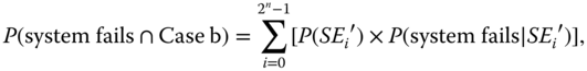
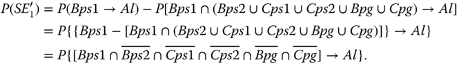
- Step 6: Evaluate P(system fails ∩ Case b) in 8.44. Under Case b, while no PFGEs occur before the failure of the trigger component, PFSEs can take place before or after the trigger component failure. Assume there are n PFSEs under Case b. If all of the PFSEs occur after the trigger failure, they are isolated (i.e. the isolation effect takes place). If at least one PFSE occurs before the trigger failure, the selective failure propagation effect takes place. To handle those effects, an event space with 2n events (denoted by SEi′) is constructed, each being a combination of occurrence or nonoccurrence of the n PFSE events before the trigger failure. Based on the total probability law, P(system fails ∩ Case b) is evaluated as
(8.46)where P(system fails | SEi′) can be obtained through the procedure similar to that for evaluating P(system fails | SEi) in step 3.
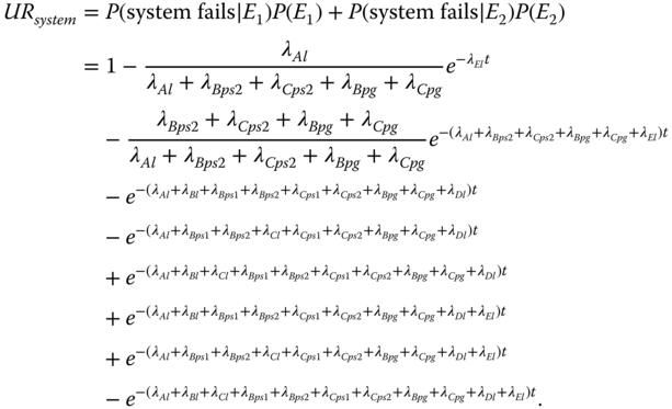
- Step 7: Integrate for final system unreliability. Based on 8.41 and 8.44, the system unreliability is calculated as
(8.47)

where P(E1) is computed at step 2, P(system fails|E1) is evaluated at step 3, P(Case a) is computed at step 5, and P(system fails ∩ Case b) is evaluated at step 6.
The above seven‐step procedure assumes that any nondependent components (including the trigger component) only undergo LFs. In the following, the procedure is extended to consider (1) PFGEs or (2) PFSEs or (3) both types of PFs for nondependent components.
- If nondependent components undergo PFGEs, the PFGE method (Section 8.2
) is applied to separate effects of PFGEs originating from the nondependent components from the overall solution combinatorics. Particularly, an additional step denoted by 8.48 is added before step 1:
(8.48)

where P'u(t) = P(no PFGEs from nondependent components), Q'(t) = P(system fails|no PFGEs from nondependent components). Q'(t) is then evaluated using the seven‐step procedure.
- If nondependent components undergo PFSEs, these PFSEs can be handled using a method similar to 8.43 before step 1. Specifically, given w independent PFSEs originating from nondependent components, an event space with 2w events is constructed, each being a combination of occurrence or nonoccurrence of the w PFSEs. The conditional system failure probability conditioned on the occurrence of each event is then evaluated using the seven‐step procedure.
- If nondependent components undergo both PFSEs and PFGEs, the process below is applied:
- As in (1), apply the PFGE method to separate effects of PFGEs originating from all the nondependent components.
- As in (2), construct an event space with 2w event combinations based on PFSEs of the nondependent components.
- Evaluate the conditional system failure probability given that each event combination occurs using the seven‐step procedure.
- Integrate the conditional system failure probabilities computed in c) to obtain Q′(t).
- Compute the final system unreliability using 8.48.
- If nondependent components undergo PFGEs, the PFGE method (Section 8.2
) is applied to separate effects of PFGEs originating from the nondependent components from the overall solution combinatorics. Particularly, an additional step denoted by 8.48 is added before step 1:
8.5.2 Case Study
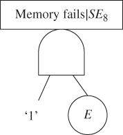
Figure 8.17 Reduced FT for P(system fails|SE8).
To evaluate P(system fails|SE8), a reduced FT is generated by replacing events of components affected by SE8 (including B, C, D) with constant 1 in the FT of Figure 8.15 , which leads to an FT containing failure events of active components {E} as shown in Figure 8.17. The evaluation of reduced FT gives
Using the similar procedure, all of P(SEi) and P(system fails|SEi) (i = 0, …, 15) can be evaluated. According to 8.43,
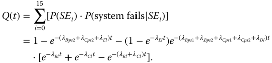
With Pu(t) and Q(t) being evaluated, according to 8.42, P(system fails|E1) is obtained as

- Step 4: Define two disjoint event cases given that E2 takes place. In the event of the trigger component A being failed, the following two cases are considered:
- Case a: At least one PFGE originating from B or C occurs before A fails.
- Case b: No PFGEs from B or C take place before A fails.
- Step 5: Evaluate P(Case a). According to 8.45, one obtains

- Step 6: Evaluate P(system fails ∩ Case b). An event space with 16 events is constructed as shown in Table 8.5.
Table 8.5 Event space for addressing PFSEs.
| i | Definition of SEi' | Set of active components |
| 0 | No PFs happen before Al occurs | {E} |
| 1 | Only Bps1 occurs before Al occurs | {E} |
| 2 | Only Bps2 occurs before Al occurs | ∅ |
| 3 | Only Cps1 occurs before Al occurs | {E} |
| 4 | Only Cps2 occurs before Al occurs | ∅ |
| 5 | Only Bps1 and Bps2 occur before Al occurs | ∅ |
| 6 | Only Bps1 and Cps1 occur before Al occurs | {E} |
| 7 | Only Bps1 and Cps2 occur before Al occurs | ∅ |
| 8 | Only Bps2 and Cps1 occur before Al occurs | ∅ |
| 9 | Only Bps2 and Cps2 occur before Al occurs | ∅ |
| 10 | Only Cps1 and Cps2 occur before Al occurs | ∅ |
| 11 | Only Bps1, Bps2 and Cps1 occur before Al occurs | ∅ |
| 12 | Only Bps1, Bps2 and Cps2 occur before Al occurs | ∅ |
| 13 | Only Bps1, Cps1 and Cps2 occur before Al occurs | ∅ |
| 14 | Only Bps2, Cps1 and Cps2 occur before Al occurs | ∅ |
| 15 | Bps1, Bps2, Cps1 and Cps2 all occur before Al occurs | ∅ |
Next the evaluation of P(SEi′) and P(system fails | SEi′) is illustrated using SE0′ and SE1′.
Under SE0′, no PF occurs before Al occurs. Thus,

where, according to 8.45
Thus,

The reduced FT for evaluating P(system fails | SE0′) is same as that in Figure 8.17
. Thus, ![]() .
.
Under SE1′, only Bps1 occurs before Al occurs. Thus,
The reduced FT for evaluating P(system fails | SE1′) is same as that in Figure 8.17
. Thus, ![]() .
.
Using the similar procedure, all of P(SEi′) and P(system fails | SEi′) (i = 0, …, 15) can be evaluated. P(system fails ∩ Case b) can thus be evaluated using 8.46. Then, according to 8.44, one obtains
- Step 7: Integrate for final system unreliability. According to 8.41, with P(E1) evaluated at step 2, P(system fails|E1) evaluated at step 3, and P(E2)P(system fails|E2) evaluated at step 6, the system unreliability considering competing failures as well as effects of both PFGEs and PFSEs is computed as:
8.6 Multi‐Phase System with Single FDEP Group
Previous sections focus on single‐phase systems. However, many real‐world systems are PMSs, involving multiple, consecutive, and nonoverlapping phases of operations or tasks. Consideration of competing failures in PMSs is a challenging task because PMSs exhibit dynamics in system configuration and component behavior, as well as statistical dependencies across phases for a given component.
This section presents a combinatorial method to address the competing failure effects in reliability analysis of nonrepairable binary‐state PMSs, where only one mission phase is subject to the FDEP behavior. As an example of such a PMS, a set of computers work together to accomplish an M‐phase mission task. In M − 1 of these phases, only local computing is needed (no FDEPs are involved), while in one of the phases, some computers need to access the Internet to access external data. Thus, in this particular phase these computers have FDEP on the router.
The phase with FDEP is referred to as an FDEP phase; other phases are referred to as non‐FDEP phases. All PFs have the global effect, i.e. only PFGEs are considered. The LF and PFGE of the same component are s‐independent. Also, failure events of different components are s‐independent. There is only one FDEP group existing in the system. Thus, the PMS considered undergoes no cascading failure propagation process.
8.6.1 Combinatorial Method
The reliability analysis method for PMSs subject to competing failure isolation and propagation effects involves the following five‐step procedure [15]:
- Step 1: Separate PFGEs of all nondependent components. Any component that cannot be isolated by the failure of another component is referred to as a nondependent component (NDC), e.g. the trigger component of an FDEP group or a component not belonging to any FDEP group. A PFGE originating from an NDC causes the failure of the entire system. Thus, the PFGE method described in Section 8.2
can be applied to separate PFGEs of all the NDCs from the solution combinatorics.
8.49

Let N denote the set of NDCs undergoing PFGEs. Pu(t) in 8.49 is evaluated as
(8.50)
As explained in Section 8.2 , the evaluation of Q(t) requires the use of a conditional LF probability for all the NDCs given that no PFGEs occur to the component during the mission. Since the LF and PFGE of the same component are s‐independent, 8.3 is applied to compute the conditional LF probability. The evaluation of Q(t) is conducted in steps 2–4.
- Step 2: Define three disjoint events E1, E2, and E3 and evaluate their probabilities. Given that no PFGEs from NDCs happen, three disjoint events are defined:
- E1: No PFGEs occur to dependent components (DCs) during the mission. Let D denote the set of DCs involved in the FDEP that undergo PFGEs. P(E1) is evaluated as
(8.51)

- E2: At least one PFGE from DCs takes place in a non‐FDEP phase. P(E2) can be evaluated as
8.52
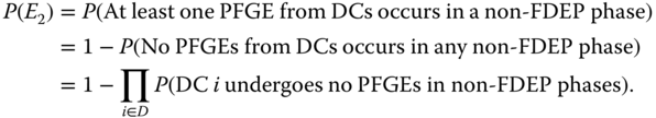
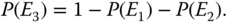
- E3: At least one PFGE from DCs occurs in the FDEP phase and no PFGEs from DCs occur in non‐FDEP phase. Because P(E1) + P(E2) + P(E3) = 1, P(E3) is evaluated as
(8.53)Based on the total probability law, Q(t) is evaluated as
 (8.54)where QiC (i = 1, 2, 3) is the conditional system failure probability given that Ei occurs and no PFGEs from the NDCs occur.
- E1: No PFGEs occur to dependent components (DCs) during the mission. Let D denote the set of DCs involved in the FDEP that undergo PFGEs. P(E1) is evaluated as
- Step 3: Evaluate Q1C and Q2C. Under E1, the PMS can be analyzed as a system without any component undergoing PFGEs. Thus, to evaluate Q1C, a reduced FT is first generated by replacing the FDEP gate with an OR gate and by considering only LFs for all the system components. The reduced FT is then evaluated using the PMS BDD method described in Section 3.5.3 [16] to obtain Q1C.
Under E2, the global failure propagation effect takes place, causing the entire system failure. Thus, Q2C = 1.
- Step 4: Evaluate
 . Under E3, competing failures can take place in the FDEP phase and the occurrence sequence of the trigger LF and PFGEs of DCs needs to be considered. Two disjoint subcases are defined under E3:
- Case 1: Failure isolation effect takes place.
The trigger LF occurs before any PFGEs from the DCs. Since under E3, all PFGEs from the DCs occur in the FDEP phase, the trigger LF occurs either in phases before the FDEP phase or in FDEP phase but before any PFGEs occurs from the DCs.
- Case 2: Failure propagation effect takes place.
The trigger LF either occurs after any PFGE from the DCs occurs or does not occur at all. Under E3, if the trigger LF occurs, the failure can only occur either in phases after the FDEP phase or in the FDEP phase but after any PFGE from the DCs occurs.
Let Q3,iC (i = 1, 2) denote the conditional system failure probability, given that Case i occurs. Based on the total probability law, one obtains
(8.55)
where Q3,2C = 1 because the global failure propagation effect takes place under Case 2.
Assume the FDEP phase is phase m. To evaluate P(Case 1) Q3,1C, an event space with m events is constructed, with event i (i = 1, …, m – 1) representing the trigger component fails locally in phase i and E3 occurs, and event m representing the trigger component fails locally in phase m (FDEP phase) and before any PFGE from the DCs occurs in phase m. Based on these events, 8.55 can be evaluated as
8.56
The occurrence probabilities of the m events are
8.57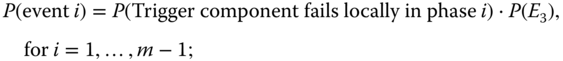 8.58
8.58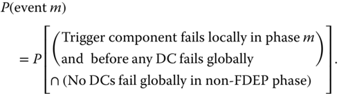
The sequential failure probability involved in 8.58 can be evaluated using integral formula 8.10, which can be solved using the MathCAD software [17].
 in 8.56 can be computed by evaluating a reduced PMS FT, which is obtained through the following procedure:
- Events in the original PMS FT in phase j (j < i) representing failure of the trigger component are replaced with constant 0 (FALSE).
- Events in phase k (k ≥ i) representing failure of the trigger component are replaced with constant 1 (TURE).
- Since at least one PFGE occurs in the FDEP phase, all DCs in the same FDEP group are affected and fail although other components outside the FDEP group are not affected by the PFGEs due to the isolation effect. Hence, events representing failures of DCs in the FDEP phase and phases after the FDEP phase are replaced with constant 1 (TURE).
- Boolean rules (1 + x = 1, 1 · x = x, 0 + x = x, 0 · x = 0, where x denotes a Boolean variable) are applied to generate the reduced FT.
The reduced FT generated is then evaluated using the PMS BDD method described in Section 3.5.3 to obtain
 .
.P(Case 2) in 8.56 can be simply computed as
(8.59)
- Case 1: Failure isolation effect takes place.
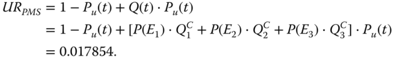
- Step 5: Integrate for final PMS unreliability. According to 8.54, P(E1) and P(E2) evaluated at step 2, Q1C and Q2C evaluated at step 3, and
 evaluated at step 4 are integrated to obtain Q(t). Further, according to 8.49, Q(t) and Pu(t) evaluated at step 1 are integrated to obtain the final PMS unreliability considering effects of competing failures.
8.6.2 Case Study
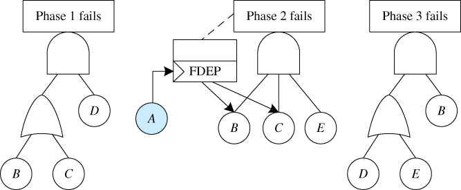
Figure 8.18 An example PMS FT.
Input Parameters. Assume the phase durations for the three phases are independent of the system state and equal to 10, 30, and 20 hours, respectively. Therefore, the entire mission time is 60 hours.
All five components experience LFs in each of the three phases. Only computers A, B, and C can undergo PFGEs during the mission (e.g. due to computer viruses). Let ![]() and
and ![]() represent the conditional probability that component x fails locally and globally at phase i, respectively, given that the component has survived the previous phase. Their complements are represented as
represent the conditional probability that component x fails locally and globally at phase i, respectively, given that the component has survived the previous phase. Their complements are represented as ![]() and
and ![]() , respectively.
, respectively.
For illustration, three types of ttf distributions are considered for evaluating ![]() and
and ![]() :
:
- Components A, B, and C have the exponential ttf distribution with constant failure rate λ given in Table 8.6. The failure probability is computed as
 , and pdf is
 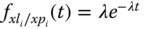 .
. - Component D has a fixed LF probability
 , i = 1, 2, 3.
 - Component E's time to LF follows the Weibull distribution with scale parameter λW and shape parameter αW given in Table 8.7. The failure probability is computed as
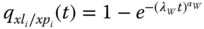 , and pdf is
Table 8.6 Failure parameters for components A, B, and C.
| Phases 1, 2, 3 | ||
| LF | PFGE | |
| A | λ = 1.5e − 4 | λ = 1e − 4 |
| B | λ = 2e − 4 | λ = 1e − 4 |
| C | λ = 2e − 4 | λ = 1e − 4 |
Table 8.7 Failure parameters for component E.
| Phase 1 | Phase 2 | Phase 3 | |
| λW | 2e − 4 | 1e − 4 | 1.5e − 4 |
| αW | 2 | 2 | 2 |
Let ![]() and
and ![]() represent the unconditional probability that component x fails locally and globally by the end of phase i, respectively.
represent the unconditional probability that component x fails locally and globally by the end of phase i, respectively. ![]() and
and ![]() can be evaluated as
can be evaluated as

Their complements are represented as ![]() and
and ![]() , respectively, and can be evaluated as
, respectively, and can be evaluated as

Example Analysis. Applying the five‐step procedure in Section 8.6.1, the unreliability of the example PMS is analyzed as follows:
- Step 1: Separate PFGEs of all nondependent components. There is only one NDC A, so Q(t) in 8.49 is evaluated as
The evaluation of Q(t) in 8.49 requires the use of a conditional LF probability for A given that no PFGEs occur to A during the mission, which is evaluated based on 8.3.
- Step 2: Define three disjoint events E1, E2, and E3 and evaluate their probabilities.
There are two DCs: B and C. Both of them can experience PFGEs. Thus, the three events are defined as:
- E1: no PFGEs occur to B and C during the entire mission. Thus,

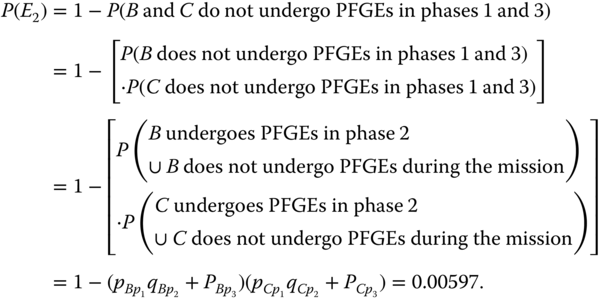
- E2: at least one PFGE from B or C takes place in non‐FDEP phases (phase 1 and phase 3). Note that component C does not appear in the phase 3 FT, meaning that its LF makes no contribution to phase 3 failure; however, its PFGE can occur and cause the entire mission failure. P(E2) is evaluated as
- E3: B or C undergoes PFGEs in the FDEP phase (phase 2), and both B and C do not undergo PFGEs in phase 1 and phase 3. P(E3) is evaluated as P(E3) = 1 − P(E1) − P(E2).
- E1: no PFGEs occur to B and C during the entire mission. Thus,
- Step 3: Evaluate Q1C and Q2C. Figure 8.19 shows the reduced FT for evaluating Q1C. The reduced FT is then evaluated using the PMS BDD method described in Section 3.5.3. Figure 8.20 shows the PMS BDD generated using the variable order of Al2 < Bl3 < Bl2 < Bl1 < Cl2 < Cl1 < Dl3 < Dl1 < El3 < El2. The evaluation of the PMS BDD model gives
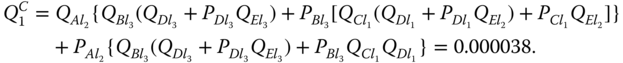

Figure 8.19 Reduced FT for evaluating Q1C.
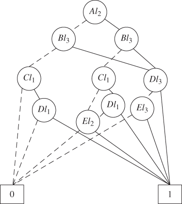
Figure 8.20 PMS BDD for Q1C.
Under E2, the global failure propagation effect from B or C occurs causing the PMS failure. Thus, Q2C = 1.
- Step 4: Evaluate
 . The two sub‐cases under E3 are
- Case 1: LF of trigger A occurs in phase 1, or occurs in phase 2 and before B or C fails globally in phase 2.
- Case 2: LF of trigger A occurs in phase 3, or occurs in phase 2 and after B or C fails globally in phase 2, or does not occur at all during the entire mission.
Under Case 1, the following two events are defined: event 1 – trigger A fails locally in phase 1 and E3 happens, event 2 – A fails locally in phase 2 and before B or C fails globally in phase 2. P(event 1) is evaluated as

To evaluate
 in 8.56, a reduced FT is generated in Figure 8.21.
Figure 8.21 Reduced FT under event 1.
Figure 8.22 shows the PMS BDD generated in the PMS BDD method using the order of Bl1 < Cl1 < Dl3 < Dl1 < El3 < El2. The evaluation of the PMS BDD model gives

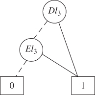
Figure 8.22 PMS BDD under event 1.
Let T2 represent the duration of phase 2. P(event 2) is evaluated as
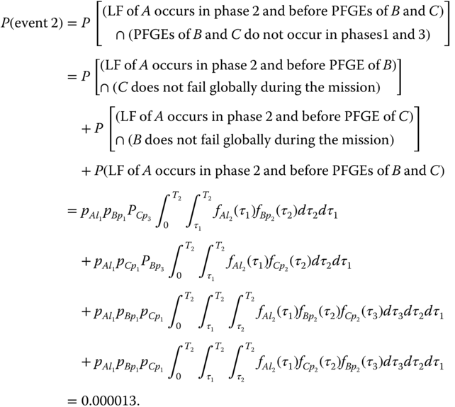
The reduced FT and PMS BDD under event 2 are the same as those under event 1. Thus,
 .
.According to 8.59, P(Case 2) in 8.56 is calculated as

According to 8.56, one obtains

- Step 5: Integrate for final PMS unreliability. According to 8.54 and 8.49, P(E1) and P(E2) evaluated at step 2, Q1C and Q2C evaluated at step 3, and
 evaluated at step 4 are integrated to obtain Q(t), which is then integrated with Pu(t) evaluated at step 1 to obtain the final PMS unreliability.
8.7 Multi‐Phase System with Multiple FDEP Groups
This section presents a continuous time Markov chain (CTMC)‐based method for modeling competing failure propagation and isolation effects in reliability analysis of PMSs with multiple FDEP groups [18]. The exponential ttf distribution is assumed for system components. The LF, PFGE, PFSE of the same component are s‐independent.
A trigger component failure in one phase, if occurring first, only makes dependent components belonging to the same FDEP group inaccessible in that phase; these dependent components are still available to use in other phases if they are accessible directly by the system function without involving the trigger component in those phases. Both PFGEs and PFSEs from the dependent component can be isolated by the trigger failure. An isolated PFGE or PFSE only affects the component itself. An isolated PFGE or PFSE in a previous phase may still propagate to other components in a later phase that does not involve operation of the related FDEP group.
8.7.1 CTMC‐Based Method
In [19] a CTMC‐based method was developed for the reliability analysis of PMSs without FDEP and related competing failures. This section presents an extension of the CTMC‐based method for considering the competing failure effects in reliability analysis of PMSs with multiple FDEP groups.
The extended CTMC‐based method involves the following three‐step procedure:
- Step 1: Develop a separate CTMC for each phase. In the traditional CTMC model [5], each component corresponds to one failure event. To consider different types of failures, each component in the extended CTMC‐based method corresponds to up to three failure events representing the occurrence of LF, PFGE, or PFSE, respectively. The initial state is a state where none of the component failure events takes place or a state where all the system components are good. Each of the subsequent states represents a combination of component LF, PFGE, and PFSE that may occur. As the failure events occur one by one, the system transits from one state to another state until the absorbing state (mission failure in a particular phase) is reached. The transition is characterized by the occurrence rate of the related component failure event.
Note that a component not appearing in a phase FT means that the LF of this component does not contribute to the mission failure in the phase. However, the PFGE or PFSE of the component can still affect the mission failure and thus should be considered for constructing the CTMC of the phase.
- Step2: Solve the CTMC of phase 1. According to (2.26), state equations of the CTMC in phase 1 are constructed. Using the initial state probabilities (1 for the initial state and 0 for all other states), the state equations can be solved using the Laplace transform method [11] .
- Step 3: Solve the CTMC for later phases. Starting from phase 2, the state probabilities evaluated for the previous phase are mapped as the initial state probabilities of the current phase CTMC for evaluation. Note that since compact CTMCs are used in each phase, some states may not exist in all of the mission phases. Consider such an example where an FDEP group exists in phase 1. The CTMC of phase 1 contains a system operation state (state x) where a PFGE has taken place in a dependent component but is isolated by the corresponding trigger failure. However, if this FDEP group does not exist in the later phase 2, then state x does not appear in the CTMC of phase 2. In this case, the system operation state x in phase 1 is mapped to the failure state in phase 2. Therefore, due to the competing failure behavior, special treatment should be taken during the phase‐to‐phase mapping process.
Repeat this step until the CTMC of all the mission phases are analyzed. The analysis of the final phase gives the final PMS unreliability. In particular, the failure state probability of the final phase is the failure probability of the entire PMS.
8.7.2 Case Study
Two examples are presented to illustrate the CTMC‐based method. The PMS in Example 8.5 contains dependent FDEP groups in different phases with dependent components undergoing LFs and PFGEs. The PMS in Example 8.6 contains dependent FDEP groups with dependent components undergoing LFs, PFGEs, and PFSEs.
8.8 Summary
In systems subject to the FDEP behavior, there exist competitions in the time domain between the failure isolation effect (caused by the trigger failure) and the failure propagation effect (caused by the PFGE/PFSE of the dependent components). As different occurrence sequences of the trigger failure and the dependent component PFGE/PFSE can lead to different system statuses, it is significant to address the competing effects in the system reliability analysis. Combinatorial methods are presented for reliability analysis of single‐phase systems with a single FDEP group or multiple dependent FDEP groups, and for multi‐phase systems with a single FDEP group. A CTMC‐based method is discussed for addressing the competing effects in the reliability analysis of multi‐phase systems with multiple FDEP groups.
References
- 1 Levitin, G. and Xing, L. (2010). Reliability and performance of multi‐state systems with propagated failures having selective effect. Reliability Engineering & System Safety 95 (6): 655–661.
- 2 Amari, S.V., Dugan, J.B., and Misra, R.B. (1999). A separable method for incorporating imperfect coverage in combinatorial model. IEEE Transactions on Reliability 48 (3): 267–274.
- 3 Levitin, G. and Amari, S.V. (2007). Reliability analysis of fault tolerant systems with multi‐fault coverage. International Journal of Performability Engineering 3 (4): 441–451.
- 4 Xing, L. and Dugan, J.B. (2002). Analysis of generalized phased‐mission systems reliability, performance and sensitivity. IEEE Transaction on Reliability 51 (2): 199–211.
- 5 Misra, K.B. (2008). Handbook of Performability Engineering. London: Springer‐Verlag.
- 6 Myers, A.F. (2007). k‐out‐of‐n: G system reliability with imperfect fault coverage. IEEE Transactions on Reliability 56 (3): 464–473.
- 7 Shrestha, A. and Xing, L. (2008). Quantifying application communication reliability of wireless sensor networks. International Journal of Performability Engineering, Special Issue on Reliability and Quality in Design 4 (1): 43–56.
- 8 Xing, L., Wang, C., and Levitin, G. (2012). Competing failure analysis in non‐repairable binary systems subject to functional dependence. Proc IMechE, Part O: Journal of Risk and Reliability 226 (4): 406–416.
- 9 Papoulis, A. (1984). Probability, Random Variables, and Stochastic Processes, 2e. New York, NY: McGraw‐Hill.
- 10 Xing, L. and Levitin, G. (2010). Combinatorial analysis of systems with competing failures subject to failure isolation and propagation effects. Reliability Engineering & System Safety 95 (11): 1210–1215.
- 11 Rausand, M. and Hoyland, A. (2003). System Reliability Theory: Models and Statistical Methods, Wiley Series in Probability and Mathematical Statistics. Wiley.
- 12 Wang, C., Xing, L., and Levitin, G. (2013). Reliability analysis of multi‐trigger binary systems subject to competing failures. Reliability Engineering & System Safety 111: 9–17.
- 13 Dugan, J.B. and Doyle, S.A. (1996). New results in fault‐tree analysis. In: Tutorial Notes of Annual Reliability and Maintainability Symposium, Las Vegas, Nevada, USA.
- 14 Wang, C., Xing, L., and Levitin, G. (2012). Propagated failure analysis for non‐repairable systems considering both global and selective effects. Reliability Engineering & System Safety 99: 96–104.
- 15 Wang, C., Xing, L., and Levitin, G. (2012). Competing failure analysis in phased‐mission systems with functional dependence in one of phases. Reliability Engineering & System Safety 108: 90–99.
- 16 Zang, X., Sun, H., and Trivedi, K.S. (1999). A BDD‐based algorithm for reliability analysis of phased‐mission systems. IEEE Transactions on Reliability 48 (1): 50–60.
- 17 Maxfield, B. (2009). Essential Mathcad for Engineering, Science, and Math, 2e. Academic Press.
- 18 Wang, C., Xing, L., Peng, R., and Pan, Z. (2017). Competing failure analysis in phased‐mission systems with multiple functional dependence groups. Reliability Engineering & System Safety 164: 24–33.
- 19 Somani, A.K., Ritcey, J.A., and Au, S.H.L. Computationally efficient phased‐mission reliability analysis for systems with variable configurations. IEEE Transactions on Reliability 41 (4): 504–511.