5
Functional Dependence
Functional dependence takes place when the malfunction of one system component (referred to as the trigger) causes other components (referred to as dependent components) within the same system to become unusable or inaccessible. For example, in a computer system, peripheral devices such as keyboards and monitors are accessed through I/O controllers. If the I/O controller malfunctions, the peripheral devices connected to it become unusable [1]. In other words, the peripheral devices have functional dependence on the I/O controller. Another example is a computer network system where a computer can access the Internet or communicate with other computers through routers [2]. The router is the trigger component, and computers connected to the router have functional dependence on the router.
The functional dependence behavior is modeled via Functional DEPendence (FDEP) gates in the dynamic fault tree (DFT) analysis [3,4] (Section 2.3.2). Note that the FDEP gate has no logical output; it is connected to the top gate of the system DFT using a dashed line. In this chapter, a logic OR replacement method is discussed for the reliability analysis of systems with FDEP and perfect fault coverage. A combinatorial approach is presented for reliability analysis of systems subject to imperfect fault coverage.
5.1 Logic OR Replacement Method
For systems with perfect fault coverage, the FDEP behavior can be addressed by replacing each FDEP gate with logic OR gates (one for each dependent component) in the system DFT model [5].
5.2 Combinatorial Algorithm
The combinatorial approach aims to successfully “turn off” the disconnected or isolated dependent components (when the corresponding trigger component fails or becomes unavailable) so that they could not contribute to the system UF probability. The approach involves four tasks that, respectively, address UFs of independent trigger components of FDEP, transform the system with FDEP into subsystems without FDEPs, evaluate resultant subsystems, and integrate for the final system unreliability.
5.2.1 Task 1: Addressing UFs of Independent Trigger Components
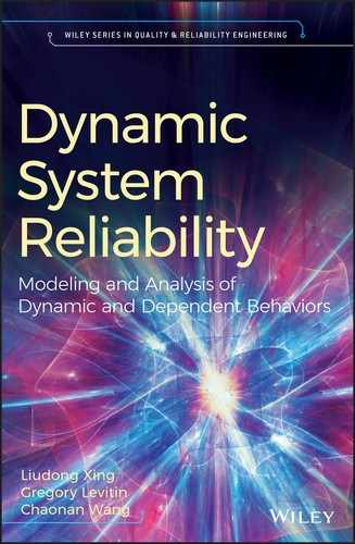
Based on the simple and efficient algorithm (SEA) (Section 3.3.2), particularly (3.4), the system unreliability is evaluated as:
Pu,IT(t) in 5.1 is the probability that no independent trigger components undergo UFs, and Q(t) is the conditional system unreliability given that no independent trigger components experiences UFs. Note that in the case of cascading FDEP appearing in the system DFT, the trigger components that also serve as dependent components (referred to as dependent trigger components) are not included in the evaluation of Pu,IT(t). According to (3.5), it is computed as
As discussed in Section 3.3.2, for each independent trigger component a conditional failure probability ![]() given that the component undergoes no UFs should be calculated and used for evaluating Q(t). According to (3.6), it is evaluated as
given that the component undergoes no UFs should be calculated and used for evaluating Q(t). According to (3.6), it is evaluated as ![]() .
.
5.2.2 Task 2: Generating Reduced Problems Without FDEP
Evaluating Q(t) in 5.1 needs to address effects of FDEP. The transformation technique developed in [21,22] is utilized to transform a reliability problem with FDEP into reduced problems without FDEP so that the SEA method can be safely applied to components that are still not disconnected or isolated.
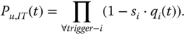
Assume the system under analysis involves m elementary independent trigger events (ITEs) (denoted by Ti, i = 1 … m). An ITE space is first built, containing 2m mutually exclusive and collectively exhaustive combined events called ITEs. Each ITE is a distinct and disjoint combination of the m elementary ITEs, illustrated as follows:
Applying the total probability law, Q(t) in 5.1 can be evaluated as:

where P(ITEi) can be evaluated based on the definition of ITEi in 5.3 and conditional occurrence probabilities of elementary trigger events involved in the definition of ![]() . Evaluating P(system fails|ITEi) in 5.4 is a reduced reliability problem, where components affected by ITEi do not appear in the system reliability model due to the occurrence of ITEi. The evaluation is detailed in Section 5.2.3.
. Evaluating P(system fails|ITEi) in 5.4 is a reduced reliability problem, where components affected by ITEi do not appear in the system reliability model due to the occurrence of ITEi. The evaluation is detailed in Section 5.2.3.
5.2.3 Task 3: Solving Reduced Reliability Problems
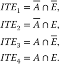
To evaluate P(system fails|ITEi), the set of components affected by ITEi (denoted by ![]() ) needs to be determined. Define a functional dependence group (FDG) as a group of components that is functionally dependent on the same trigger event. For example, components B, D, and F in Figure 5.1
a form the FDG for component A, denoted as FDGA = {B, D, F}. The set
) needs to be determined. Define a functional dependence group (FDG) as a group of components that is functionally dependent on the same trigger event. For example, components B, D, and F in Figure 5.1
a form the FDG for component A, denoted as FDGA = {B, D, F}. The set ![]() is determined as the union of all FDGs whose corresponding trigger event takes place when ITEi happens.
is determined as the union of all FDGs whose corresponding trigger event takes place when ITEi happens.
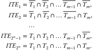
For example, consider an FDEP system with two elementary ITEs T1 and T2. The ITE space constructed contains ![]() ,
, ![]() ,
, ![]() , ITE4 = T1 ∩ T2. For event
, ITE4 = T1 ∩ T2. For event ![]() (the occurrence of ITE1 implies that neither T1 nor T2 occurs), set
(the occurrence of ITE1 implies that neither T1 nor T2 occurs), set ![]() is simply an empty set (no components are affected). For event
is simply an empty set (no components are affected). For event ![]() (the occurrence of ITE2 implies the occurrence of T2 only), set
(the occurrence of ITE2 implies the occurrence of T2 only), set ![]() is simply
is simply ![]() . For event
. For event ![]() (the occurrence of ITE3 implies the occurrence of T1 only), set
(the occurrence of ITE3 implies the occurrence of T1 only), set ![]() is simply
is simply ![]() . For event ITE4 = T1 ∩ T2 (the occurrence of ITE4 implies the occurrence of T1 and T2), set
. For event ITE4 = T1 ∩ T2 (the occurrence of ITE4 implies the occurrence of T1 and T2), set ![]() is the union of
is the union of ![]() ,
, ![]() , and
, and ![]() . Note that
. Note that ![]() is applicable and must be included when T1 ∩ T2 serves as a trigger input of some FDEP gate in the system DFT.
is applicable and must be included when T1 ∩ T2 serves as a trigger input of some FDEP gate in the system DFT.
5.2.3.1 Expansion Process
In the case of cascading FDEP appearing in the system DFT, the set ![]() should be expanded to include all basic events following the domino chain of dependent events involved. The expansion process is iterative. During each iteration, if the input trigger event condition of an FDEP gate is satisfied by any combination of components already in
should be expanded to include all basic events following the domino chain of dependent events involved. The expansion process is iterative. During each iteration, if the input trigger event condition of an FDEP gate is satisfied by any combination of components already in ![]() , all the dependent basic events of the corresponding FDEP gate should be added to the expanded set. The expansion process ends when no new components are added to the set
, all the dependent basic events of the corresponding FDEP gate should be added to the expanded set. The expansion process ends when no new components are added to the set ![]() after the previous iteration. Refer to Section 5.5 for an example of applying this expansion process.
after the previous iteration. Refer to Section 5.5 for an example of applying this expansion process.
With ![]() being identified, a reduced FT model is generated for the reduced problems P(system fails|ITEi) based on the original DFT using the following procedure.
being identified, a reduced FT model is generated for the reduced problems P(system fails|ITEi) based on the original DFT using the following procedure.
5.2.3.2 Reduced FT Generation Procedure
- Remove all the ITEs and related FDEP gates from the original system DFT.
- Replace basic failure events of components appearing in set
 in the original system DFT by constant logic value 1 (True). After the replacement, all the components affected by ITEi disappear from the system model. Consequently, they can be successfully “turned off” so that their UFs (if there are any) are not able to contribute to the system failure.
 - Apply Boolean algebra (0 + x = x, 1 + x = 1, 0 · x = 0, 1 · x = x) to simplify the DFT after the replacement.
5.2.3.3 Dual Trigger‐Basic Event Handling
Note that in the case of an event playing dual roles (particularly, the event being a trigger event of certain FDEP gate and a basic event of other gates at the same time), in step 1 of the above reduced FT generation procedure, only the trigger event identity of a dual event is removed while its basic event identity stays. In step 2, the dual event's basic event identity is replaced by constant logic value 1 (True) when the event itself (e.g. T1) appears in ITEi; or by constant logic value 0 (False) when the complement of the event (e.g. ![]() ) appears in ITEi. If the basic event identity appears as an input of a logic AND gate and it is replaced by 0, and the other input of the AND gate undergoes UFs, Boolean algebra particularly, 0 · x = 0 in step 3 cannot be applied so that the UFs can be considered for evaluating P(system fails|ITEi). Refer to Section 5.6 for an illustration of applying this special handling procedure to a system with dual events.
) appears in ITEi. If the basic event identity appears as an input of a logic AND gate and it is replaced by 0, and the other input of the AND gate undergoes UFs, Boolean algebra particularly, 0 · x = 0 in step 3 cannot be applied so that the UFs can be considered for evaluating P(system fails|ITEi). Refer to Section 5.6 for an illustration of applying this special handling procedure to a system with dual events.
5.2.3.4 Evaluation of P(system fails|ITEi)
Based on the reduced FT generated, if no FDEP remains, the SEA method (Section 3.3.2) is applied to address UFs of the remaining components connected to the system model (i.e. components not affected by ITEi). Equation (5.5) shows the evaluation of P(system fails|ITEi) by applying (3.4).
where Pu, i(t) = ∏∀cc−k(1 − sk · qk(t)) is the probability that no connected components (cc) undergo UFs. Qi(t) in 5.5 is the system unreliability ignoring all the UFs and effects of FDEP; its evaluation requires modifying each cc's failure probability to a conditional probability computed as ![]() (based on (3.6)).
(based on (3.6)).
However, the reduced FT for P(system fails|ITEi) may still contain FDEP gate(s) when the cascading FDEP behavior appears in the original DFT. In this case, Tasks 1–3 need to be repeated for evaluating P(system fails|ITEi). Specifically, UFs of the ITEs in the reduced FT (they are actually dependent trigger events in the original DFT) are first separated from the solution combinatorics using the SEA methodology (Task 1). The ITE space is then built based on those ITEs of the reduced FT (Task 2). Each reduced problem is solved using the SEA method in the case of no further FDEP existing in the reduced FT generated or using steps of Tasks 1–3 when any FDEP still remains.
5.2.4 Task 4: Integrating to Obtain Final System Unreliability
After evaluating all of the reduced problems, the final system unreliability considering effects of both IPC and FDEP is obtained by applying 5.4 and 5.1, consecutively.
5.2.5 Algorithm Summary
A systematic algorithm based on the combinatorial approach detailed in the preceding subsections 5.2.1–5.2.4 is summarized as follows:
- Find all the elementary ITEs in the FT considered and perform the following computations:
- Compute Pu, IT = ∏∀trigger−i(1 − si · qi(t)).
- Compute
 for each independent trigger component i.
- Construct the ITE space 5.3 with 2m disjoint ITEs in the case of m elementary ITEs existing in the FT considered.
- For each ITEi,
- Compute P(ITEi) using conditional failure probabilities of trigger components computed in step 1.b.
- Identify set
 .
. - Build the reduced FT model for P(system fails|ITEi) using the generation procedure presented in Section 5.2.3.2.
- If the reduced FT contains no further FDEP gates, then
- Compute Pu, i = ∏∀cc−k(1 − sk · qk(t));
- Compute
 for each cc (i.e. component appearing in the reduced FT generated in step 3.c;
 - Evaluate the reduced FT model generated in step 3.c by applying the BDD‐based method (Section 2.4) to obtain Qi (
 is used for evaluating Qi);
 - According to 5.5, compute P(system fails|ITEi) = 1 − Pu, i + Pu, i · Qi.
- If the reduced FT contains further FDEP gates, then go back to step 1 and repeat the evaluation procedure based on this reduced FT until P(system fails|ITEi) is evaluated.
- According to 5.4, compute
 (in the case of cascading FDEPs, this step may also generate Qi).
 - According to 5.1, compute URsystem = 1 − Pu, IT + Pu, IT · Q (in the case of cascading FDEPs, this step may also generate P(system fails|ITEi)).
5.2.6 Algorithm Complexity
Step 3 of the algorithm in Section 5.2.5 dominates the complexity of the entire algorithm, involving O(2M) reduced reliability problems to be solved using any traditional FT reliability analysis method, where M represents the number of trigger components (including independent and dependent) [3] . The BDD‐based method adopted was shown to require less memory and be computationally more efficient than other FT reliability analysis methods [ 3 ,8, 9 ,23,24]. Particularly, applying the dynamic programming [25] concept of memoization, the computational complexity of the BDD model evaluation is O(number of non‐sink nodes in BDD). Refer to [26] for a detailed storage and computation complexity analysis of an efficient BDD implementation method.
As illustrated through case studies in Sections 5.3– 5.6 , the reduced reliability problems generated are simplified and independent problems, which could be solved concurrently given available computing resources.
The combinatorial algorithm is applicable to arbitrary types of component ttf distributions. It is also computationally more efficient than the CTMC‐based method. The number of states (or state equations) in the CTMC model is w = O(2n) (exponential to the number of components n, usually far greater than the number of trigger components M). The computational time for solving a Markov model with w‐states is O(w3) [27].
Note that in [21]
a combinatorial method was suggested for handling FDEP in IPC systems, which can handle noncascading FDEP accurately. However, in the case of cascading FDEP, the trigger components that also simultaneously serve as dependent components (i.e. dependent trigger components) cannot be isolated or turned off appropriately in the algorithm of [21]
; their UFs can always contribute to the system failure, leading to overestimated system unreliability results. But the algorithm of [21]
is still more accurate than the logic OR replacement method for handling cascading FDEP systems because it can always isolate the purely dependent components (without the trigger role) appropriately. The algorithm presented in this section improves the method of [21]
through handling the trigger events involved in cascading FDEP in a hierarchical manner. By doing so, both dependent trigger components and purely dependent components can be turned off appropriately during the evaluation process.
5.3 Case Study 1: Combined Trigger Event
Figure 5.2 illustrates the DFT model of the memory subsystem for a computer system [17,28]. The memory subsystem has five memory units Mi (i = 1, 2, 3, 4, 5); they are accessible through two memory interface units (MIU1, MIU2). In other words, the memory units have FDEP on the MIUs (elementary trigger events). Particularly, as illustrated in the DFT, the following FDEP relationships exist in the system:
- M1 and M2 are connected to the system bus via MIU1; M1 and M2 are functionally dependent on MIU1 (i.e. FDGMIU1 = {M1, M2}).
- M3 is connected to both interfaces implying that M3 is accessible as long as one of the two interface units is functioning, or when both interface units malfunction M3 becomes inaccessible. M3 is functionally dependent on MIU1 ∩ MIU2, which is referred to as a combined trigger event (i.e. FDGMIU1∩MIU2 = {M3}).
- M4 and M5 are connected to the system bus via MIU2; M4 and M5 are functionally dependent on MIU2 (i.e. FDGMIU2 = {M4, M5}).

Figure 5.2 DFT of an example memory system [ 17 , 28 ].
Table 5.1 presents five distinct sets of failure rates and coverage factors for components of the memory subsystem. The r factor is assumed to be ZERO for all the system components. Mission time of t = 10 000 hours is considered.
Table 5.1 Input component failure parameters (/hr) and coverage factors.
| Set 1 | Set 2 | Set 3 | Set 4 | Set 5 | |
| λMIU1, λMIU2 | 1e−6 | 1e−6 | 1e−6 | 1e−6 | 1e−6 |
| λMi, i = 1, 2, ..., 5 | 1e−4 | 1e−4 | 1e−4 | 1e−4 | 1e−4 |
| cMIUi, i = 1, 2 | 1 | 0.9 | 1 | 1 | 1 |
| cM1 | 0.9 | 0.9 | 0.5 | 1 | 1 |
| cM2 | 0.9 | 0.9 | 0.5 | 1 | 1 |
| cM3 | 0.9 | 0.9 | 0.5 | 0.5 | 1 |
| cM4 | 0.9 | 0.9 | 1 | 0.5 | 1 |
| cM5 | 0.9 | 0.9 | 1 | 0.5 | 1 |
Applying the combinatorial method, an ITE space with four ITEs is constructed:
Their occurrence probabilities are evaluated as:

where ![]() . In the case of an exponential distribution for ttf of MIU, qMIUi = 1 − exp(−λMIUi · t) for i = 1, 2. Values of P(ITEi) are shown in Table 5.2.
. In the case of an exponential distribution for ttf of MIU, qMIUi = 1 − exp(−λMIUi · t) for i = 1, 2. Values of P(ITEi) are shown in Table 5.2.
Table 5.2 Occurrence probabilities of ITEs.
| Set 1 | Set 2 | Set 3 | Set 4 | Set 5 | |
| P(ITE1) | 0.980199 | 0.982152 | 0.980199 | 0.980199 | 0.980199 |
| P(ITE2) | 9.85116e−3 | 8.883714e−3 | 9.85116e−3 | 9.85116e−3 | 9.85116e−3 |
| P(ITE3) | 9.85116e−3 | 8.883714e−3 | 9.85116e−3 | 9.85116e−3 | 9.85116e−3 |
| P(ITE4) | 9.90058e−5 | 8.035453e−5 | 9.90058e−5 | 9.90058e−5 | 9.90058e−5 |
Further, ![]() ,
, ![]() ,
, ![]() , and
, and ![]() are determined. Next reduced FT models are generated to evaluate P(system fails|ITEi). Apparently, P(system fails|ITE4) = 1 for all the five different parameter settings. Figure 5.3 shows the reduced FTs for the first three reduced problems. Based on the evaluation of these reduced FTs (using the BDD‐based method) and 5.5, P(system fails|ITEi) are obtained as shown in Table 5.3.
are determined. Next reduced FT models are generated to evaluate P(system fails|ITEi). Apparently, P(system fails|ITE4) = 1 for all the five different parameter settings. Figure 5.3 shows the reduced FTs for the first three reduced problems. Based on the evaluation of these reduced FTs (using the BDD‐based method) and 5.5, P(system fails|ITEi) are obtained as shown in Table 5.3.
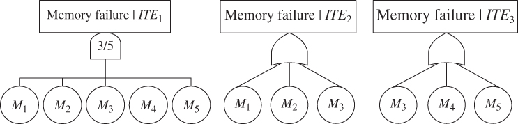
Figure 5.3 Reduced FT models.
Table 5.3 Evaluation results of P(system fails|ITEi) and Q.
| Set 1 | Set 2 | Set 3 | Set 4 | Set 5 | |
| P(system fails|ITE1) | 0.780023 | 0.780023 | 0.858244 | 0.858244 | 0.736436 |
| P(system fails|ITE2) | 0.950212 | 0.950212 | 0.950212 | 0.950212 | 0.950212 |
| P(system fails|ITE3) | 0.950212 | 0.950212 | 0.950212 | 0.950212 | 0.950212 |
| P(system fails|ITE4) | 1 | 1 | 1 | 1 | 1 |
| Q | 0.783398 | 0.783064 | 0.860070 | 0.860070 | 0.740674 |
According to 5.4, P(ITEi) and P(system fails|ITEi) are integrated to obtain Q (last row of Table 5.3 ). Lastly, according to 5.1 the final system unreliability is obtained. Table 5.4 presents values of the final system unreliability evaluated. It also presents the system unreliability analyzed using the logic OR replacement method. For parameters sets 1–4, the logic OR replacement method generates overestimated system unreliability. For parameter set 5, the two methods generate identical results because the dependent memory units experience no UFs (the c factor is ONE).
Table 5.4 Final system unreliability.
| Approaches | Set 1 | Set 2 | Set 3 | Set 4 | Set 5 | |
| Combinatorial | 0.783398 | 0.783496 | 0.86007 | 0.86007 | 0.740674 | |
| Logic OR | 0.783518 | 0.783604 | 0.860331 | 0.860331 | 0.740674 | |
Since no cascading FDEPs are involved in this case study, the algorithm of [21] can generate results that are identical to those of the combinatorial algorithm presented in this section. If the CTMC‐based method is applied to analyze this example memory system, a compact CTMC model (after merging all system failed states and related transitions) containing 87 states and 190 transitions [17] has to be solved. In contrast, the combinatorial method involves only solving three static FTs with five, three, and three components, respectively (Figure 5.3 ).
5.4 Case Study 2: Shared Dependent Event
Figure 5.4 illustrates the DFT of an example system with dependent event C shared by two FDEP gates. Table 5.5 gives five sets of input component failure parameters and coverage factors. All the system components have exponential ttf distributions. The r factor is assumed to be ZERO for all the system components. Mission time of t = 10 000 hours is considered.
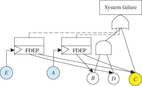
Figure 5.4 Example system with shared dependent events.
Table 5.5 Input component failure parameters and coverage factors.
| Set 1 | Set 2 | Set 3 | Set 4 | Set 5 | |
| λA | 1e−5 | 1e−5 | 1e−5 | 1e−5 | 1e−5 |
| λB,C,D,E | 1e−5 | 1e−4 | 1e−4 | 1e−4 | 1e−4 |
| cA | 0.9 | 0.9 | 0.9 | 0.9 | 1 |
| cB | 0.9 | 0.9 | 0.5 | 0.9 | 1 |
| cC | 0.9 | 0.9 | 0.5 | 0.9 | 1 |
| cD, cE | 1 | 1 | 1 | 0.9 | 1 |
The ITE space contains four ITEs:
Their occurrence probabilities are:

Values of P(ITEi) are shown in Table 5.6. Further, ![]() ,
, ![]() ,
, ![]() , and
, and ![]() are obtained. Applying the reduced FT generation procedure in Section 5.2.3
, the reduced FT model for P(system fails|ITE1) is obtained in Figure 5.5. P(system fails|ITEi) for i = 2, 3, and 4 is simply constant 1, meaning that the system always fails when the corresponding ITEi occurs.
are obtained. Applying the reduced FT generation procedure in Section 5.2.3
, the reduced FT model for P(system fails|ITE1) is obtained in Figure 5.5. P(system fails|ITEi) for i = 2, 3, and 4 is simply constant 1, meaning that the system always fails when the corresponding ITEi occurs.
Table 5.6 Occurrence probabilities of ITEs.
| Set 1 | Set 2 | Set 3 | Set 4 | Set 5 | |
| P(ITE1) | 0.826597 | 0.336069 | 0.336069 | 0.358746 | 0.332871 |
| P(ITE2) | 0.086934 | 0.577462 | 0.577462 | 0.554785 | 0.571966 |
| P(ITE3) | 0.078241 | 0.03181 | 0.03181 | 0.033957 | 0.035008 |
| P(ITE4) | 0.008229 | 0.054659 | 0.054659 | 0.052512 | 0.060154 |

Figure 5.5 Reduced FT model.
Based on the evaluation of the reduced FT in Figure 5.5 and 5.5, P(system fails|ITE1) is obtained as shown in Table 5.7. According to 5.4, P(ITEi) in Table 5.6 and P(system fails| ITEi) in Table 5.7 are integrated to obtain Q (last row of Table 5.7 ). Lastly, according to 5.1, the final system unreliability is obtained. Table 5.8 presents values of the final system unreliability evaluated. It also presents the system unreliability analyzed using the logic OR replacement method. The final system unreliability results obtained using the two methods are identical for this case study. The reason is that when either of the two trigger events (A or E) happens, the entire system fails. In this case, whether the disconnected dependent components can be turned off (in the combinatorial method) or not (in the logic OR replacement method) does not matter.
Table 5.7 Evaluation results of P(system fails|ITEi) and Q.
| Set 1 | Set 2 | Set 3 | Set 4 | Set 5 | |
| P(system fails|ITE1) | 0.111148 | 0.787671 | 0.821891 | 0.796226 | 0.779117 |
| P(system fails|ITE2) | 1 | 1 | 1 | 1 | 1 |
| P(system fails|ITE3) | 1 | 1 | 1 | 1 | 1 |
| P(system fails|ITE4) | 1 | 1 | 1 | 1 | 1 |
| Q | 0.265278 | 0.928643 | 0.940143 | 0.926897 | 0.926474 |
Table 5.8 Final system unreliability.
| Approaches | Set 1 | Set 2 | Set 3 | Set 4 | Set 5 |
| Combinatorial | 0.27227 | 0.929322 | 0.940713 | 0.93217 | 0.926474 |
| Logic OR | 0.27227 | 0.929322 | 0.940713 | 0.93217 | 0.926474 |
Since no cascading FDEP is involved in this case study, the algorithm of [21] can generate results that are identical to those of the combinatorial algorithm presented in this section. If the CTMC‐based method is applied to analyze the example system with a shared dependent event, a compact CTMC model (after merging all system failed states and related transitions) containing four states and five transitions (Figure 5.6) has to be solved. In contrast, the combinatorial method presented in Section 5.2 involves solving only one static FT with three components (Figure 5.5 ).

Figure 5.6 CTMC for the example system (F: system failure).
5.5 Case Study 3: Cascading FDEP
The cascading behavior occurs when the failure of one component in the system results in a chain reaction or domino effect [29]. Consider a hierarchical hub network where its nodes and hubs are organized into multiple levels. A node at lower levels can be accessible via multiple hubs of different levels. If the top‐level hub undergoes a failure, then all its child or grandchild hubs and nodes connected to these hubs become inaccessible in a cascading manner [30]. Cascading effects can be modeled using multiple cascading FDEP gates in the DFT model.
Figure 5.7 illustrates the DFT model of a system with a two‐stage domino chain behavior, modeled using two cascading FDEP gates. When event A occurs, both events B and E are forced to occur; consequently, event C also occurs due to the occurrence of event B. In this example system, event A is an ITE while event B is a dependent trigger event. Five sets of input parameters in Table 5.9 are considered. It is assumed that all the system components fail exponentially with identical constant failure rate λA,B,C,D,E,F = 1e−5/hour. The r factor is assumed to be ZERO for all the system components. Mission time of t = 10 000 hours is used for the analysis.

Figure 5.7 An example system with cascading FDEP.
Table 5.9 Input component coverage factors.
| Set 1 | Set 2 | Set 3 | Set 4 | Set 5 | |
| cA | 0.9 | 0.9 | 0.9 | 1 | 1 |
| cB | 0.9 | 0.9 | 0.9 | 0.8 | 1 |
| cC | 0.9 | 0.9 | 1 | 1 | 1 |
| cD | 1 | 0.9 | 1 | 1 | 1 |
| cE | 0.9 | 0.9 | 1 | 1 | 1 |
| cF | 1 | 0.9 | 1 | 1 | 1 |
Applying the algorithm in Section 5.2.5
, since there is a single ITE A in the original system DFT, one obtains Pu, IT = 1 − sA · qA(t) and ![]() , where qA(t) = 1 − exp(−λA · t). An ITE space with two ITEs is then constructed:
, where qA(t) = 1 − exp(−λA · t). An ITE space with two ITEs is then constructed: ![]() , ITE2 = A. Their occurrence probabilities are:
, ITE2 = A. Their occurrence probabilities are: ![]() ,
, ![]() . Values of P(ITEi) are shown in Table 5.10.
. Values of P(ITEi) are shown in Table 5.10.
Table 5.10 Occurrence probabilities of ITEs.
| Set 1 | Set 2 | Set 3 | Set 4 | Set 5 | |
| P(ITE1) | 0.913531 | 0.913531 | 0.913531 | 0.904837 | 0.904837 |
| P(ITE2) | 0.086469 | 0.086469 | 0.086469 | 0.095163 | 0.095163 |
Further, ![]() and
and ![]() are obtained. Note that the “Expansion Process” for cascading FDEP described in Section 5.2.3.1 is applied to generate
are obtained. Note that the “Expansion Process” for cascading FDEP described in Section 5.2.3.1 is applied to generate ![]() . Specifically, the set
. Specifically, the set ![]() not only includes events B and E (which are directly dependent on A) but also should be expanded to include event C. Figure 5.8 gives FT models of the two reduced problems P(system fails|ITE1) and P(system fails|ITE2).
not only includes events B and E (which are directly dependent on A) but also should be expanded to include event C. Figure 5.8 gives FT models of the two reduced problems P(system fails|ITE1) and P(system fails|ITE2).
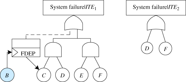
Figure 5.8 Reduced FT models.
5.5.1 Evaluation of P(system fails|ITE1)
As the FT model for P(system fails|ITE1) contains an FDEP gate, the combinatorial algorithm needs to be recursively applied to evaluate P(system fails|ITE1). Specifically, since there is a single ITE B in the reduced FT, one obtains Pu, IT = 1 − sB · qB(t) and ![]() , where qB(t) = 1 − exp(−λB · t). An ITE space with two ITEs is then constructed for evaluating P(system fails|ITE1):
, where qB(t) = 1 − exp(−λB · t). An ITE space with two ITEs is then constructed for evaluating P(system fails|ITE1): ![]() , ITE1, 2 = B. Their occurrence probabilities are evaluated as:
, ITE1, 2 = B. Their occurrence probabilities are evaluated as: ![]() ,
, ![]() as shown in Table 5.11.
as shown in Table 5.11.
Table 5.11 Occurrence probabilities of ITEs for evaluating P(system fails|ITE1).
| Set 1 | Set 2 | Set 3 | Set 4 | Set 5 | |
| P(ITE1,1) | 0.913531 | 0.913531 | 0.913531 | 0.922393 | 0.904837 |
| P(ITE1,2) | 0.086469 | 0.086469 | 0.086469 | 0.077607 | 0.095163 |
Further, ![]() and
and ![]() are obtained. Figure 5.9 gives FT models of the two reduced problems P(system fails|ITE1,1) and P(system fails|ITE1,2). Since both of the reduced FTs are free of FDEP gates, the SEA method, i.e. Eq. (5.5) is applicable to evaluating the reduced problems. Table 5.12 presents the evaluation results for the five sets of input parameters. Using 5.4, P(system fails|ITE1,1) and P(system fails|ITE1,2) can then be integrated with P(ITE1,1) and P(ITE1,2) in Table 5.11
to find Q(t), which is further combined with Pu, IT = 1 − sB · qB(t) using 5.1 to find P(system fails|ITE1). The last row of Table 5.12
shows the evaluation results for P(system fails|ITE1).
are obtained. Figure 5.9 gives FT models of the two reduced problems P(system fails|ITE1,1) and P(system fails|ITE1,2). Since both of the reduced FTs are free of FDEP gates, the SEA method, i.e. Eq. (5.5) is applicable to evaluating the reduced problems. Table 5.12 presents the evaluation results for the five sets of input parameters. Using 5.4, P(system fails|ITE1,1) and P(system fails|ITE1,2) can then be integrated with P(ITE1,1) and P(ITE1,2) in Table 5.11
to find Q(t), which is further combined with Pu, IT = 1 − sB · qB(t) using 5.1 to find P(system fails|ITE1). The last row of Table 5.12
shows the evaluation results for P(system fails|ITE1).
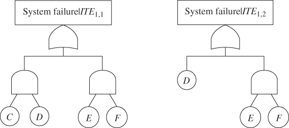
Figure 5.9 Reduced FT models for evaluating P(system fails|ITE1).
Table 5.12 Evaluation results of P(system fails|ITE1,i) and P(system fails|ITE1).
| Set 1 | Set 2 | Set 3 | Set 4 | Set 5 | |
| P(system fails|ITE1,1) | 0.035021 | 0.051864 | 0.018030 | 0.018030 | 0.018030 |
| P(system fails|ITE1,2) | 0.111148 | 0.118939 | 0.103357 | 0.103357 | 0.103357 |
| P(system fails|ITE1) | 0.050724 | 0.066631 | 0.034682 | 0.043215 | 0.026150 |
5.5.2 Evaluation of P(system fails|ITE2)
As the FT model for P(system fails|ITE2) is free of FDEP gates, the SEA method, i.e. Eq. (5.5) is directly applicable to evaluating P(system fails|ITE2). Specifically, Pu,2(t) = (1 − sD · qD(t))(1 − sF · qF(t)), ![]() , and
, and ![]() . Further Q2(t) =
. Further Q2(t) = ![]() . Based on 5.5, Pu,2(t) and Q2(t) are combined to obtain P(system fails|ITE2). Table 5.13 presents the evaluation results.
. Based on 5.5, Pu,2(t) and Q2(t) are combined to obtain P(system fails|ITE2). Table 5.13 presents the evaluation results.
Table 5.13 Evaluation results of P(system fails|ITE2).
| Set 1 | Set 2 | Set 3 | Set 4 | Set 5 | |
| Pu,2(t) | 1 | 0.981058 | 1 | 1 | 1 |
| Q2(t) | 0.181269 | 0.165461 | 0.181269 | 0.181269 | 0.181269 |
| P(system fails|ITE2) | 0.181269 | 0.181269 | 0.181269 | 0.181269 | 0.181269 |
5.5.3 Evaluation of URsystem
According to 5.4, P(ITEi) in Table 5.10 , P(system fails|ITE1) (last row of Table 5.12 ) and P(system fails|ITE2) (last row of Table 5.13 ) are integrated to obtain Q(t), which is further combined with Pu, IT = 1 − sA · qA(t) using 5.1 to obtain the final system unreliability. Table 5.14 presents values of the final system unreliability evaluated using the combinatorial algorithm. It also presents the system unreliability analyzed using the algorithm of [21] and the logic OR replacement method. For parameter sets 1–4, the algorithm of [21] and the logic OR replacement method both give overestimated system unreliability results. For sets 1 and 2, results obtained using the algorithm of [21] are closer to the accurate results because the purely dependent components C and E can be turned off appropriately in the algorithm of [21] , but not in the logic OR replacement method. For sets 3 and 4, the algorithm of [21] and the logic OR replacement method give identical results because the purely dependent components C and E undergo no UFs (the c factor being 1); the dependent trigger component B undergoes UFs but cannot be turned off in both methods. For parameter set 5, the three methods give identical results because none of the dependent trigger component (B) and the purely dependent components (C and E) experience UFs; thus, they do not require the “turn‐off” function.
Table 5.14 Final system unreliability.
| Set 1 | Set 2 | Set 3 | Set 4 | Set 5 | |
| Combinatorial | 0.070938 | 0.085333 | 0.056423 | 0.056353 | 0.040911 |
| Algorithm [21] | 0.071605 | 0.085999 | 0.057090 | 0.057835 | 0.040911 |
| Logic OR | 0.073576 | 0.087964 | 0.057090 | 0.057835 | 0.040911 |
5.6 Case Study 4: Dual Event and Cascading FDEP
Consider an example of systems involving both cascading FDEP and dual trigger‐basic events in Figure 5.10. Specifically, T1 and T2 are dual events (trigger events for FDEP and basic events contributing to the two AND gates at the same time). All the system components fail exponentially with constant failure rates (/hour) λA = 2e − 5, λB = 1e − 5, λT1 = 1e − 4, and λT2 = 1e − 5. Five sets of coverage factors in Table 5.15 are considered. The r factor is assumed to be ZERO for all the system components. Mission time of t = 10 000 hours is used for the analysis.
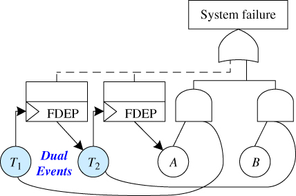
Figure 5.10 An example system containing cascading FDEP and dual events.
Table 5.15 Input component coverage factors.
| Set 1 | Set 2 | Set 3 | Set 4 | Set 5 | |
| cA | 0.9 | 0.9 | 0.9 | 0.95 | 1 |
| cB | 0.9 | 1 | 1 | 0.9 | 1 |
| cT1 | 0.9 | 1 | 1 | 0.9 | 1 |
| cT2 | 0.9 | 1 | 0.9 | 1 | 1 |
Applying the algorithm in Section 5.2.5
, since there is a single ITE T1 in the original system DFT, one obtains ![]() and
and ![]() , where
, where ![]() . An ITE space with two ITEs is then constructed:
. An ITE space with two ITEs is then constructed: ![]() , ITE2 = T1. Their occurrence probabilities are:
, ITE2 = T1. Their occurrence probabilities are: ![]() ,
, ![]() . Values of P(ITEi) are shown in Table 5.16.
. Values of P(ITEi) are shown in Table 5.16.
Table 5.16 Occurrence probabilities of ITEs.
| Set 1 | Set 2 | Set 3 | Set 4 | Set 5 | |
| P(ITE1) | 0.392703 | 0.367879 | 0.367879 | 0.392703 | 0.367879 |
| P(ITE2) | 0.607297 | 0.632121 | 0.632121 | 0.607297 | 0.632121 |
Further, ![]() and
and ![]() are obtained. Note that the “Expansion Process” for cascading FDEP described in Section 5.2.3.1
is applied to generate
are obtained. Note that the “Expansion Process” for cascading FDEP described in Section 5.2.3.1
is applied to generate ![]() . Specifically, the set
. Specifically, the set ![]() not only includes event T2 (which is directly dependent on T1) but also should be expanded to include event A. Figure 5.11 gives FT models of the two reduced problems P(system fails|ITE1) and P(system fails|ITE2). Since T1 is a dual event, the special handling procedure in Section 5.2.3.3 is applied to generate the reduced FT for P(system fails|ITE1), where only the trigger event identity of T1 is removed while its basic event identity stays and is replaced by constant logic value 0 (as
not only includes event T2 (which is directly dependent on T1) but also should be expanded to include event A. Figure 5.11 gives FT models of the two reduced problems P(system fails|ITE1) and P(system fails|ITE2). Since T1 is a dual event, the special handling procedure in Section 5.2.3.3 is applied to generate the reduced FT for P(system fails|ITE1), where only the trigger event identity of T1 is removed while its basic event identity stays and is replaced by constant logic value 0 (as ![]() appears in ITE1). The reduced FT for P(system fails|ITE2) is simply constant 1 after applying the Boolean algebra reduction.
appears in ITE1). The reduced FT for P(system fails|ITE2) is simply constant 1 after applying the Boolean algebra reduction.
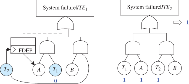
Figure 5.11 Reduced FT models.
5.6.1 Evaluation of P(system fails|ITE1)
As the FT model for P(system fails|ITE1) contains an FDEP gate, the combinatorial algorithm needs to be recursively applied to evaluate P(system fails|ITE1). Specifically, since there is a single ITE T2 in the reduced FT, one obtains ![]() and
and ![]() , where
, where ![]() . An ITE space with two ITEs is then constructed for evaluating P(system fails|ITE1):
. An ITE space with two ITEs is then constructed for evaluating P(system fails|ITE1): ![]() , ITE1, 2 = T2. Their occurrence probabilities are evaluated as:
, ITE1, 2 = T2. Their occurrence probabilities are evaluated as: ![]() ,
, ![]() as shown in Table 5.17.
as shown in Table 5.17.
Table 5.17 Occurrence probabilities of ITEs for evaluating P(system fails|ITE1).
| Set 1 | Set 2 | Set 3 | Set 4 | Set 5 | |
| P(ITE1,1) | 0.913531 | 0.904837 | 0.913531 | 0.904837 | 0.904837 |
| P(ITE1,2) | 0.086469 | 0.095163 | 0.086469 | 0.095163 | 0.095163 |
Further, ![]() and
and ![]() are obtained. Figure 5.12 gives FT models of the two reduced problems P(system fails|ITE1,1) and P(system fails|ITE1,2). Since both of the reduced FTs are free of FDEP gates, the SEA method, i.e. Eq. (5.5) is directly applicable to evaluating the reduced problems. Table 5.18 presents the evaluation results for the five sets of input parameters. Note that in the reduced FT for P(system fails|ITE1,1), the Boolean algebra 0 · x = 0 cannot be applied because UFs of A and B can still contribute to the system failure (since they are not isolated). When applying the SEA method, Pu,1,1(t) = (1 − sAqA(t))·(1 − sBqB(t)) and Q1,1(t) = 0. Applying 5.5, one obtains P(system fails|ITE1,1) = 1 − Pu,1,1(t) representing the probability that at least one of the two components A and B undergoes a UF.
are obtained. Figure 5.12 gives FT models of the two reduced problems P(system fails|ITE1,1) and P(system fails|ITE1,2). Since both of the reduced FTs are free of FDEP gates, the SEA method, i.e. Eq. (5.5) is directly applicable to evaluating the reduced problems. Table 5.18 presents the evaluation results for the five sets of input parameters. Note that in the reduced FT for P(system fails|ITE1,1), the Boolean algebra 0 · x = 0 cannot be applied because UFs of A and B can still contribute to the system failure (since they are not isolated). When applying the SEA method, Pu,1,1(t) = (1 − sAqA(t))·(1 − sBqB(t)) and Q1,1(t) = 0. Applying 5.5, one obtains P(system fails|ITE1,1) = 1 − Pu,1,1(t) representing the probability that at least one of the two components A and B undergoes a UF.

Figure 5.12 Reduced FT models for evaluating P(system fails|ITE1).
Table 5.18 Evaluation results of P(system fails|ITE1,i) and P(system fails|ITE1).
| Set 1 | Set 2 | Set 3 | Set 4 | Set 5 | |
| P(system fails|ITE1,1) | 0.027471 | 0.018127 | 0.018127 | 0.018493 | 0.000000 |
| P(system fails|ITE1,2) | 0.095163 | 0.095163 | 0.095163 | 0.095163 | 0.095163 |
| P(system fails|ITE1) | 0.042523 | 0.025458 | 0.034069 | 0.025790 | 0.009056 |
Using 5.4, P(system fails|ITE1,1) and P(system fails|ITE1,2) can then be integrated with P(ITE1,1) and P(ITE1,2) in Table 5.17
to find Q(t), which is further combined with ![]() using 5.1 to find P(system fails|ITE1). The last row of Table 5.18
shows the evaluation results for P(system fails|ITE1).
using 5.1 to find P(system fails|ITE1). The last row of Table 5.18
shows the evaluation results for P(system fails|ITE1).
5.6.2 Evaluation of URsystem
According to 5.4, P(ITEi) in Table 5.16
, P(system fails|ITE1) (last row of Table 5.18
) and P(system fails|ITE2) = 1 are integrated to obtain Q(t), which is further combined with ![]() using 5.1 to obtain the final system unreliability. Table 5.19 presents values of the final system unreliability evaluated using the combinatorial algorithm. It also presents the system unreliability analyzed using the logic OR replacement method.
using 5.1 to obtain the final system unreliability. Table 5.19 presents values of the final system unreliability evaluated using the combinatorial algorithm. It also presents the system unreliability analyzed using the logic OR replacement method.
Table 5.19 Final system unreliability.
| Set 1 | Set 2 | Set 3 | Set 4 | Set 5 | |
| Combinatorial | 0.647764 | 0.641486 | 0.644654 | 0.641608 | 0.635452 |
| Logic OR | 0.648281 | 0.642060 | 0.645170 | 0.641895 | 0.635452 |
For parameter sets 1–4, the logic OR replacement method generates overestimated system unreliability results; for parameter set 5 (all the system components experience no UFs), the two methods give identical results. In the case of all the system components having exponential ttf distributions, this example system can be analyzed using the CTMC‐based method. A compact Markov chain as shown in Figure 5.13 must be solved, which contains 6 states and 11 transitions. In contrast, the combinatorial method presented in this chapter involves only analyzing the two reduced FTs in Figure 5.12 .

Figure 5.13 CTMC for the example system with dual events.
5.7 Summary
This chapter discusses methods for reliability analysis of systems subject to the FDEP behavior. The logic OR replacement method is only applicable to systems with perfect fault coverage, but generates overestimated system unreliability results for systems with imperfect fault coverage. The algorithm presented in [21] works perfectly for IPC systems subject to noncascading FDEPs, but generates overestimated system unreliability results in the case of the occurrence of cascading FDEPs in the system. The combinatorial algorithm described in Section 5.2 can handle various complicated cases including cascading FDEPs, combined trigger events, shared dependent events, and dual‐role events. The algorithm, which practices the divide and conquer principle based on the total probability law, is computationally efficient. The reduced reliability problems generated are simplified and independent problems without FDEP, which can be solved in parallel given available computing resources using any traditional FT analysis method.
The methods explained in this chapter do not address possible competitions existing between a covered failure of a trigger component and UFs of the corresponding dependent components. Refer to Chapters 8 and 9 for models and methods of addressing deterministic and probabilistic competing effects, respectively.
References
- 1 Stallings, W. (2009). Computer Organization and Architecture, 8e. Prentice Hall.
- 2 Xing, L., Levitin, G., Wang, C., and Dai, Y. (2013). Reliability of systems subject to failures with dependent propagation effect. IEEE Transactions Systems, Man, and Cybernetics: Systems 43 (2): 277–290.
- 3 Dugan, J.B. and Doyle, S.A. (1996). New results in fault‐tree analysis. In: Tutorial Notes of Annual Reliability and Maintainability Symposium. Las Vegas, Nevada, USA.
- 4 Dugan, J.B., Bavuso, S.J., and Boyd, M.A. (1992). Dynamic fault‐tree models for fault‐tolerant computer systems. IEEE Transactions on Reliability 41 (3): 363–377.
- 5 Merle, G., Roussel, J‐M., and Lesage, J‐J. (2010). Improving the efficiency of dynamic fault tree analysis by considering gates FDEP as static. In: Proceeding of European Safety and Reliability Conference. Rhodes, Greece.
- 6 Misra, K.B. (2008). Handbook of Performability Engineering. London: Springer‐Verlag.
- 7 Bryant, R.E. (1986). Graph‐based algorithms for Boolean function manipulation. IEEE Transactions on Computers 35 (8): 677–691.
- 8 Rauzy, A. (1993). New algorithms for fault tree analysis. Reliability Engineering and System Safety 40: 203–211.
- 9 Zang, X., Sun, H., and Trivedi, K.S. (1999). A BDD‐based algorithm for reliability analysis of phased‐mission systems. IEEE Transactions on Reliability 48 (1): 50–60.
- 10 Bouricius, W.G., Carter, W.C., and Schneider, P.R. (1969). Reliability modeling techniques for self‐repairing computer systems. In: Proceedings of 24th Ann. ACM., National Conference, 295–309, New York, NY, USA.
- 11 Arnold, T.F. (1973). The concept of coverage and its effect on the reliability model of a repairable system. IEEE Transactions on Computers C‐22: 325–339.
- 12 Levitin, G. and Amari, S.V. (2007). Reliability analysis of fault tolerant systems with multi‐fault coverage. International Journal of Performability Engineering 3 (4): 441–451.
- 13 Myers, A.F. (2007). k‐out‐of‐n: G system reliability with imperfect fault coverage. IEEE Transactions on Reliability 56 (3): 464–473.
- 14 Myers, A.F. (2008). Achievable limits on the reliability of k‐out‐of‐n: G systems subject to imperfect fault coverage. IEEE Transactions on Reliability 57: 349–354.
- 15 Dugan, J.B. (1991). Automated analysis of phased‐mission reliability. IEEE Transactions on Reliability 40 (1): 45–52,55.
- 16 Gulati, R. and Dugan, J.B. (1997). A modular approach for analyzing static and dynamic fault trees. In: Proceedings of the Annual Reliability and Maintainability Symposium. Philadelphia, PA, USA.
- 17 Manian, R., Dugan, J.B., Coppit, D., and Sullivan, K.J. (1998). Combining various solution techniques for dynamic fault tree analysis of computer systems. In: Proceedings of the 3rd IEEE International High‐Assurance Systems Engineering Symposium, 21–28. Washington, DC, USA.
- 18 Meshkat, L., Xing, L., Donohue, S., and Ou, Y. (2003). An overview of the phase‐modular fault tree approach to phased‐mission system analysis. In: Proceedings of The International Conference on Space Mission Challenges for Information Technology. Pasadena, CA, USA.
- 19 Sune, V. and Carrasco, J.A. (1997). A method for the computation of reliability bounds for non‐repairable fault‐tolerant systems In: Proceedings of the 5th IEEE International Symposium on Modeling, Analysis, and Simulation of Computers and Telecommunication System, 221–228. Haifa, Israel.
- 20 Sune, V. and Carrasco, J.A. (2001). A failure‐distance based method to bound the reliability of non‐repairable fault‐tolerant systems without the knowledge of minimal cutsets. IEEE Transactions on Reliability 50 (1): 60–74.
- 21 Xing, L., Morrissette, B.A., and Dugan, J.B. (2014). Combinatorial reliability analysis of imperfect coverage systems subject to functional dependence. IEEE Transactions on Reliability 63 (1): 367–382.
- 22 Xing, L. (2008). Handling functional dependence without using Markov models. International Journal of Performability Engineering, Short Communications 4 (1): 95–97.
- 23 Xing, L. and Dugan, J.B. (2002). Analysis of generalized phased mission system reliability, performance and sensitivity. IEEE Transactions on Reliability 51 (2): 199–211.
- 24 Chang, Y., Amari, S.V., and Kuo, S. (2004). Computing system failure frequencies and reliability importance measures using OBDD. IEEE Transactions on Computers 53 (1): 54–68.
- 25 Cormen, T.H., Leiserson, C.E., Rivest, R.L., and Stein, C. (2001). Introduction to Algorithms, 2e. MIT Press.
- 26 Brace, K.S., Rudell, R.L., and Bryant, R.E. (1990). Efficient implementation of a BDD package In: Proceedings of the 27th ACM/IEEE Design Automation Conference, 40–45. Orlando, FL, USA.
- 27 Reibman, A., Smith, R., and Trivedi, K.S. (1989). Markov and Markov reward model transient analysis: an overview of numerical approaches. European Journal of Operational Research 40 (2): 257–267.
- 28 Dugan, J.B., Venkataraman, B., and Gulati, R. (1997). DIFtree: A software package for the analysis of dynamic fault tree models. In: Proceedings of the Annual Reliability and Maintainability Symposium, 64–70. Philadelphia, PA, USA.
- 29 Rausand, M. and Hoyland, A. (2003). System Reliability Theory: Models and Statistical Methods, Wiley Series in Probability and Mathematical Statistics. Wiley.
- 30 Davari, S. and Zarandi, M.H.F. (2013). The single‐allocation hierarchical hub‐median problem with fuzzy flows. In: Proceedings of the 5th International Workshop Soft Computing Applications, 165–181.