9.4. Handset and Channel Distortion

Because of the proliferation of e-banking and e-commerce, recent research on speaker verification has focused on verifying speakers' identity over the phone. A challenge of phone-based speaker verification is that transducer variability could result in acoustic mismatches of the speech data gathered from different handsets. The recent popularity of mobile and Internet phones further complicates the problem, because speech coders in these phones also introduce acoustic distortion to the speech signals. The sensitivity to handset variations and speech coding algorithms means that handset compensation techniques are essential for practical speaker verification systems.

This section describes several compensation techniques to resolve the channel mismatch problems. These techniques combine handset selectors [352-354] with stochastic feature and model transformation [226, 227, 394] to reduce the acoustic mismatch between different handsets and different speech coders. Coder-dependent GMM-based handset selectors [397, 398] are trained to identify the most likely handset used by the claimants. Stochastic feature and model transformations are then applied to remove the acoustic distortion introduced by the coder and the handset. Experimental results show that the proposed technique outperforms conventional approaches and significantly reduces error rates under seven different coders (G.711, G.726, GSM, G.729, G.723.1, MELP, and LPC) with bit rates ranging from 2.4Kbps to 64Kbps. Strong correlation between speech quality and verification performance has also been observed.

9.4.1. Handset and Channel Compensation Techniques

Current approaches to handset and channel compensation can be divided into feature transformation and model transformation. The former transforms the distorted speech features to fit the clean speaker models, whereas the latter adapts or transforms the parameters of the clean models to fit the distorted speech. These two types of compensation approaches are discussed next.

Feature Transformation

As mentioned before, one of the key problems in phone-based speaker verification is the acoustic mismatch between speech gathered from different handsets. One possible approach to resolving the mismatch problem is feature transformation. Feature-based approaches attempt to modify the distorted features so that the resulting features fit the clean speech models better. These approaches include cepstral mean subtraction (CMS) [13] and signal bias removal [294], which approximate a linear channel by the long-term average of distorted cepstral vectors. These approaches, however, do not consider the effect of background noise. A more general approach, in which additive noise and convolutive distortion are modeled as codeword-dependent cepstral biases, is codeword-dependent cepstral normalization (CDCN) [3]. The CDCN, however, works well only when the background noise level is low.

When stereo corpora are available, channel distortion can be estimated directly by comparing the clean feature vectors against their distorted counterparts. For example, in SNR-dependent cepstral normalization (SDCN) [3], cepstral biases for different signal-to-noise ratios are estimated in a maximum-likelihood framework. In probabilistic optimum filtering [261], the transformation is a set of multidimensional least-squares filters whose outputs are probabilistically combined. These methods, however, rely on the availability of stereo corpora. The requirement of stereo corpora can be avoided by making use of the information embedded in the clean speech models. For example, in stochastic matching [332], the transformation parameters are determined by maximizing the likelihood of the clean models given the transformed features.

Model Transformation

Instead of transforming the distorted features to fit the clean speech model, the clean speech models can be modified such that the density functions of the resulting models fit the distorted data better. This is known as model-based transformation in the literature. Influential model-based approaches include (1) stochastic matching [332] and stochastic additive transformation [317], where the models' means and variances are adjusted by stochastic biases; (2) maximum-likelihood linear regression (MLLR) [200], where the mean vectors of clean speech models are linearly transformed; and (3) constrained reestimation of Gaussian mixtures [78], where both mean vectors and covariance matrices are transformed. Recently, MLLR has been extended to maximum-likelihood linear transformation [110], in which the transformation matrices for the variances can be different from those for the mean vectors. Meanwhile, the constrained transformation noted in Digalakis et al. [78] has been extended to piecewise-linear stochastic transformation [76], where a collection of linear transformations is shared by all the Gaussians in each mixture. The random bias shown by Sankar and Lee [332] has also been replaced by a neural network to compensate for nonlinear distortion [344]. All of these extensions show improvement in recognition accuracy.

Because the preceding methods "indirectly" adjust the model parameters via a small number of transformations, they may not be able to capture the fine structure of the distortion. Although this limitation can be overcome by the Bayesian techniques [157, 197], where model parameters are adjusted "directly," the Bayesian approach requires a large amount of adaptation data to be effective. Because both direct and indirect adaptations have their own strengths and weaknesses, a natural extension is to combine them so that the two approaches can complement each other [252, 341].

Limitations of Current Approaches

Although the preceding methods have been successful in reducing channel mismatches, most of them operate on the assumption that the channel effect can be approximated by a linear filter. Most phone handsets, in fact, exhibit energy-dependent frequency responses [308] for which a linear filter may be a poor approximation. Recently, this problem has been addressed by considering the distortion as a nonlinear mapping [205, 291]. However, these methods rely on the availability of stereo corpora with accurate time alignment.

To address these limitations, the Mak and Kung [226] and Mak et al. [227] studies proposed a method in which nonlinear transformations can be estimated under a maximum-likelihood framework, thus eliminating the need for accurately aligned stereo corpora. The only requirement is to record a few utterances generated by a few speakers using different handsets. These speakers need not utter the same set of sentences during the recording sessions, although this may improve the system's performance. The nonlinear transformation technique is detailed in the next section.

9.4.2. Stochastic Feature Transformation

The stochastic feature transformation (SFT) technique is inspired by the stochastic matching method of Sankar and Lee [332]. Stochastic matching was originally proposed for speaker adaptation and channel compensation. Its main goal is to transform the distorted data to fit the clean speech models or to transform the clean speech models to better fit the distorted data. In the case of feature transformation, the channel is represented by either a single cepstral bias (b = [b₁, b₂, ..., b_D]^T) or a bias together with an affine transformation matrix (A = diag {a₁, a₂, ..., a_D}). In the latter case, the componentwise form of the transformed vectors is given by

Equation 9.4.1

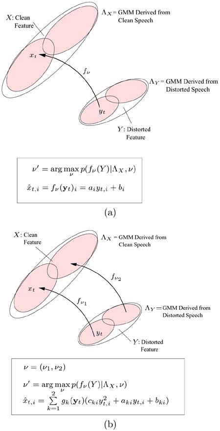
where y_t is a D-dimensional distorted vector, is the set of transformation parameters, and f_v(·) denotes the transformation function. Intuitively, the bias b compensates the convolutive distortion and the matrix A compensates the effects of noise. Figure 9.4(a) illustrates the concept of stochastic feature transformation with a single set of linear transformation parameters v per handset.

The first-order transformation in Eq. 9.4.1, however, has two limitations. First, it assumes that all speech signals are subject to the same degree of distortion, which may be incorrect for nonlinear channels where signals with higher amplitude are subject to a higher degree of distortion, because of the saturation effect in transducers. Second, the use of a single transformation matrix is inadequate for an acoustic environment with varying noise levels. A new approach to overcome these limitations is proposed next.

Nonlinear Feature Transformation

The proposal is based on the notion that different transformation matrices and bias vectors can be applied to transform the vectors in different regions of the feature space. This can be achieved by extending Eq. 9.4.1 to

Equation 9.4.2

where v = {a_ki, b_ki, c_ki; k = 1, …, K; i = 1, …, D} is the set of transformation parameters and

Equation 9.4.3

is the posterior probability of selecting the k-th transformation given the distorted speech y_t. Note that the selection of transformation is probabilistic and data-driven. In Eq. 9.4.3, is the speech model that characterizes the distorted speech and

Equation 9.4.4

is the density of the k-th distorted cluster. Figure 9.4(b) illustrates the idea of nonlinear feature transformation with different transformations for different regions of the feature space. Note that when K = 1 and c_ki = 0, Eq. 9.4.2 is reduced to Eq. 9.4.1 (i.e., the standard stochastic matching is a special case of the proposed approach).

Given a clean speech model derived from the clean speech of several speakers (10 speakers in this work), the maximum-likelihood estimates of v can be obtained by maximizing an auxiliary function

Equation 9.4.5

with respect to v'. In Eq. 9.4.5, v' and v represent the new and current estimates of the transformation parameters, respectively. T is the number of distorted vectors; denotes the k-th transformation; is the determinant of the Jacobian matrix, the (r, s)-th entry of which is given by ; and h_j(f_v(y_t)) is the posterior probability given by

Equation 9.4.6

where

Equation 9.4.7

Ignoring the terms independent of v' and assuming diagonal covariance (i.e., = diag , and likewise for ), Eq. 9.4.5 can be written as

Equation 9.4.8

The generalized EM algorithm can be applied to find the maximum-likelihood estimates of v. Specifically, in the E-step, Eqs. 9.4.6 and 9.4.7 are used to compute h_j(f_v(y_t)) and Eqs. 9.4.3 and 9.4.4 are used to compute g_k(y_t); then in the M-step, v' is updated according to

Equation 9.4.9

where η (= 0.001 in this work) is a positive learning factor and ∂Q(v'|v)/∂v' is the derivative of Q(v'|v) with respect to , that is,

Equation 9.4.10

Equation 9.4.11

Equation 9.4.12

These E- and M-steps are repeated until Q(v'|v) ceases to increase. In this work, Eq. 9.4.9 was repeated 20 times in each M-step.

The posterior probabilities g_k(y_t) and h_j(f_v(y_t)) suggest that there are K regions in the distorted feature space and M regions in the clean feature space. As a result, there are KM possible transformations; however, this number can be reduced to K by arranging the indexes j and k such that the symmetric divergence

between the j-th mixture of Λ_x and the k-th mixture of Λ_y is minimal.

Piecewise Linear Feature Transformation

When c_ji = 0, Eq. 9.4.2 becomes a piecewise linear version of the standard stochastic matching in Eq. 9.4.1. The maximum-likelihood estimate of v can be obtained by the EM algorithm. Specifically, in the M-step, the derivative of Eq. 9.4.8 with respect to v' is set to 0, which results in

Equation 9.4.13

where

where h_tj ≡ h_j(f_v(y_t)) and g_tk ≡ g_k(y_t) are estimated during the E-step.

Justification for Using Second-Order Transformation

Research has shown that handset distortion is the major source of recognition errors [131], that different handsets cause different degrees of distortion of speech signals [253], and that distortion can be nonlinear [308, 393]. As a result, the probability density functions of the distorted cepstra caused by different handsets are different. A set of GMMs can be used to estimate the probability that the observed speech comes from a particular handset.

To compare the characteristics of Eqs. 9.4.1 and 9.4.2, Gaussian noise was added to a section of switchboard conversations x(n) and the resulting signals were passed through a bandpass filter with cutoff frequencies at 625Hz and 1,875Hz. The resulting signals were subsequently passed through a nonlinear function f (x) − tanh(7x), where x was normalized to (−0.25, +0.25) to obtain a distorted signal y(n). Figure 9.5 depicts the projection of the cepstral coefficients obtained at different stages of processing on the first two components cl − c2. Evidently, the Gaussian noise shrinks the clean cluster (□), suggesting that at least one affine transformation matrix is needed. The bandpass filter shifts the noise-corrupted cluster (*) to another region of the feature space, which explains the inclusion of the bias terms b_i in Eqs. 9.4.1 and 9.4.2. The nonlinear filter twists the bandpass filtered cluster (○) and moves it closer to the clean cluster. This suggests the necessity of using more than one affine transformation matrix.

Figure 9.6 depicts the cluster recovered by Eq. 9.4.1, and Figure 9.7 illustrates how the linear regressor in Eq. 9.4.1 solves the regression problem. A closer look at Figure 9.7 reveals that the amount of componentwise variation in the clean and distorted speech is almost identical. This suggests that a single regressor is inadequate. Figure 9.8 plots the clean cluster, the distorted cluster, and the cluster recovered by the second-order transformation in Eq. 9.4.2. Figure 9.9 illustrates how the nonlinear probabilistic regressors solve the problem. These figures show that the nonlinear regressors are better than the linear ones in fitting the data. In particular, Figure 9.8 shows that almost none of the recovered data falls outside the region of the clean cluster. Evidently, having more than one nonlinear regressor for each component helps reduce transformation error.

Handset Selector

Unlike speaker adaptation in which the adapted system is used by the same "adapted" speaker in all subsequent sessions, speaker verification allows the claimant to be a different person during each verification session. As a result, the claimant's speech cannot be used for adaptation because doing so would transform the claimant's speech to fit the client model in the case of feature transformation (or transform the client model to fit the claimant's speech in the case of model adaptation). This results in verification error if the claimant turns out to be an impostor. Therefore, instead of using the claimant speech for determining the transformation parameters or adapting the client model directly, it can be used indirectly as follows.

Before verification takes place, one set of transformation parameters (or adaptation parameters) is obtained for each type of handset that the clients are likely to use. During verification, the most likely handset to be used by the claimant is identified and the best set of transformation parameters is selected accordingly. Specifically, during verification an utterance of the claimant's speech is fed to H GMMs—denoted as . The most likely handset is selected according to

Equation 9.4.14

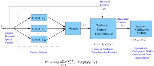
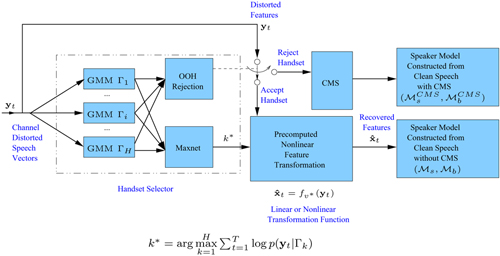
where p(y_t|Г_k) is the likelihood of the k-th handset. Finally, the transformation parameters corresponding to the k*-th handset are used to transform the distorted vectors. Figure 9.10 illustrates the idea of combining a handset selector with feature transformation in a speaker verification system (see p. 314).

Experimental Evaluations

Evaluation of HTIMIT Speech

The HTIMIT corpus [304] was used to evaluate the feature transformation approach. HTIMIT was constructed by playing a gender-balanced subset of the TIMIT corpus through nine phone handsets and a Sennheizer head-mounted microphone. Unlike other phone speech databases, where no handset labels are given, every utterance in HTIMIT is labeled with a handset name (cb1-cb4, e11-el4, pt1, or senh). This feature makes HTIMIT amenable to the study of transducer effects in speech and speaker recognition. Because of this special characteristic, HTIMIT has been used in several speaker recognition studies, including Mak et al. [227] and Quartieri et al. [289].

Speakers in the corpus were divided into a speaker set (50 male and 50 female) and an impostor set (25 male and 25 female). Each speaker was assigned a personalized 32-center GMM (with diagonal covariance) that models the characteristics of his or her own voice. For each GMM, the feature vectors derived from the SA and SX sentence sets of the corresponding speaker were used for training. A collection of all SA and SX sentences uttered by all speakers in the speaker set was used to train a 64-center GMM background model (M_b). The feature vectors were 12th order LP-derived cepstral coefficients computed at a frame rate of 71Hz using a Hamming window of 28ms.

For each handset in the corpus, the SA and SX sentences of 10 speakers were used to create two 2-center GMMs (Λx and Λy in Figure 9.4).^[5] For each handset, a set of feature transformation parameters v were computed based on the estimation algorithms described in Section 9.4.2. Specifically, the utterances from the handset "senh" were used to create ΛX, and those from the other 9 handsets were used to create Λy₁, …, Λy₉. The number of transformations for all handsets was set to 2 (i.e., K = 2 in Eq. 9.4.2).

^[5] Only a few speakers will be sufficient for creating these models; however, no attempt was made to determine the optimum number.

During verification, a vector sequence Y derived from a claimant's utterance (SI sentence) was fed to a GMM-based handset selector described in the Handset Selector section. A set of transformation parameters was selected according to the handset selector's outputs (Eq. 9.4.14). The features were transformed and then fed to a 32-center GMM speaker model (M_S) to obtain a score (log p(Y|M_s)), which was then normalized according to

Equation 9.4.15

where M_b is a 64-center GMM background model. S(Y) was compared against a threshold to make a verification decision. In this work, the threshold for each speaker was adjusted to determine an EER (i.e., speaker-dependent thresholds were used). Similar to Mak and Kung [225] and Reynolds and Rose [307] studies, the vector sequence was divided into overlapping segments to increase the resolution of the error rates.

Table 9.5 compares different stochastic feature transformation approaches against CMS and the baseline (without any compensation). All error rates were based on the average of 100 genuine speakers and 50 impostors. Evidently, all cases of stochastic feature transformation show significant reduction in error rates. In particular, second-order stochastic transformation achieves the highest reduction. The second last column of Table 9.5 shows that when the enrollment and verification sessions use the same handset (senh), CMS can degrade the performance. On the other hand, in the case of feature transformation (rows 3 to 8), the handset selector can detect the fact that the claimant is using the enrollment handset. As a result, the error rates become very close to the baseline. This suggests that the combination of handset selector and stochastic transformation can maintain the performance under matched conditions.

Table 9.5. EERs achieved by the baseline, CMS, and different transformation approaches. Note: STO, ST1, and ST2 stand for stochastic transformation with zero- first-, and second-order, respectively; the enrollment handset is senh. The second last column represents the case where enrollment and verification use the same handset. The average handset identification accuracy is 98.29%. Note that the baseline and CMS do not require the handset selector. The value of K in column 2 represents the range of summation in Eq. 9.4.2. Ave. stands for the average EER of the ten handsets.

Row	Transformation Method	Equal Error Rate (%)
		cb1	cb2	cb3	cb4	ell	e12	e13	e14	pt1	senh	Ave.
1	Baseline	7.89	6.93	26.96	18.53	5.79	14.09	7.80	13.85	9.51	2.98	11.43
2	CMS	5.81	5.02	12.07	9.41	5.26	8.88	8.44	6.90	6.97	3.58	7.23
3	STO, K = 1	4.06	3.63	8.86	6.05	3.57	6.78	6.66	4.79	5.43	2.99	5.28
4	STO, K = 2	4.27	3.74	9.19	6.74	3.68	6.95	7.06	5.00	5.38	3.09	5.51
5	ST1, K = 1	4.33	4.06	8.92	6.26	4.30	7.44	6.39	4.83	6.32	3.47	5.63
6	ST1, K = 2	4.27	3.84	9.14	6.73	3.83	7.01	6.98	5.04	5.74	3.16	5.57
7	ST2, K = 1	4.10	3.65	8.98	6.06	3.63	6.94	7.23	4.87	5.41	3.03	5.93
8	ST2, K = 2	4.04	3.57	8.85	6.82	3.53	6.43	6.41	4.76	5.02	2.98	5.24

Evaluation of Transcoded HTIMIT Speech

To evaluate the performance of the feature transformation technique on the coded HTIMIT corpora, seven codecs were employed in this work: G.711 at 64kpss, G.726 at 32Kbps, GSM at 13Kbps, G.729 at 8Kbps, G.723.1 at 6.3Kbps, MELP at 2.4Kbps, and LPC at 2.4Kbps. Six sets of coded corpora were obtained by coding the speech in HTIMIT using these coders. The encoded utterances were then decoded to produce resynthesized speech. Feature vectors were extracted from each of the utterances in the uncoded and coded corpora. The feature vectors were twelfth-order mel-frequency cepstral coefficients (MFCC) [69]. These vectors were computed at a frame rate of 14ms using a Hamming window of 28ms.

Six handset selectors, each consisting of 10 GMMs {; i = 1, …, 6 and k = 1, …, 10}, were constructed from the SA and SX sentence sets of the coded corpora. For example, GMM represents the characteristics of speech derived from the k-th handset of the i-th coded corpus. Assuming that in most practical situations the receiver will know the type of coders being used (otherwise it will not be able to decode the speech), there will not be any error in choosing the handset selector. The only error that will be introduced is the incorrect decisions made by the chosen handset selector. This error, however, is very small, as demonstrated in the latter part of this section.

During verification, a vector sequence Y derived from a claimant's utterance (SI sentence) was fed to a coder-dependent handset selector corresponding to the coder being used by the claimant. According to the outputs of the handset selector (Eq. 9.4.14), a set of coder-dependent transformation parameters was selected. The experimental results are summarized in Tables 9.6, 9.7, and 9.8. A baseline experiment (without using the handset selectors and feature transformations) and an experiment using CMS as channel compensation were also conducted for comparison. All error rates are based on the average of 100 genuine speakers, with each speaker impersonated by 50 impostors.

Table 9.6. EERs achieved by the baseline approach. Note: Results are without handset selectors and feature transformation on speech corpora coded by different coders.

Codec	Equal Error Rate (%)
	cb1	cb2	Cb3	cb4	ell	e12	e13	e14	pt1	senh	Ave.
Uncoded (128Kbps)	4.85	5.67	21.19	16.49	3.60	11.11	5.14	11.56	11.74	1.26	9.26
G.711 (64Kbps)	4.88	5.86	21.20	16.73	3.67	11.08	5.21	12.28	12.04	1.34	9.43
G.726 (32Kbps)	6.36	8.71	22.67	19.61	6.83	14.98	6.68	16.81	16.42	2.66	12.17
GSM (13Kbps)	6.37	6.10	19.90	15.93	6.21	17.93	9.86	15.29	16.42	2.35	11.64
G.729 (SKbps)	6.65	4.59	20.15	15.08	6.18	14.28	6.71	9.63	11.93	2.67	9.79
G.723.1 (6.3Kbps)	7.33	5.49	20.83	15.59	6.56	14.71	6.58	10.63	14.03	3.30	10.51
MELP (2.4Kbps)	8.56	7.36	24.99	19.71	7.48	16.13	7.17	16.97	13.31	3.23	12.49
LPC (2.4Kbps)	10.81	10.30	29.68	24.21	8.56	19.29	10.56	19.19	14.97	3.43	15.10

Table 9.7. EERs achieved by the CMS approach on speech corpora coded by different coders.

Codec	Equal Error Rate (%)
	cb1	cb2	cb3	cb4	ell	e12	e13	e14	pt1	senh	Ave.
Uncoded (128Kbps)	4.00	3.02	10.69	6.62	3.36	5.16	5.67	4.05	5.67	3.67	5.19
G.711 (64Kbps)	4.06	3.07	10.73	6.70	3.43	5.26	5.74	4.23	5.84	3.75	5.28
G.726 (32Kbps)	5.65	4.42	11.78	8.00	5.61	7.95	6.97	6.47	9.07	5.12	7.10
GSM (13Kbps)	5.25	4.10	11.32	8.00	4.95	7.04	7.47	6.05	7.58	4.73	6.65
G.729 (8Kbps)	5.43	4.37	11.81	7.98	5.16	7.38	7.32	5.42	7.21	4.69	6.68
G.723.1 (6.3Kbps)	6.40	4.60	12.36	8.53	6.11	8.50	7.31	6.11	8.28	5.62	7.38
MELP (2.4Kbps)	5.79	4.81	13.72	8.75	5.13	8.18	7.31	6.40	7.93	5.86	7.39
LPC (2.4Kbps)	6.34	5.51	14.10	9.22	6.35	8.95	8.95	6.34	9.55	4.57	7.99

Table 9.8. EERs achieved by combining zero-order feature transformation with coder-dependent handset selectors on speech corpora coded by different coders. The accuracy achieved by the handset selectors is also shown. "HS Acc." stands for handset identification accuracy.

Codec	Equal Error Rate (%)											HS Acc. (%)
	cb1	cb2	cb3	cb4	ell	e12	e13	e14	pt1	senh	Ave.
Uncoded (128Kbps)	1.63	1.27	9.65	4.47	1.41	3.58	3.37	1.66	3.08	1.09	3.12	98.13
G.711 (64Kbps)	1.52	1.26	9.57	4.53	1.41	3.53	3.33	1.72	3.21	1.17	3.13	98.22
G.726 (32Kbps)	2.55	2.55	11.66	6.05	2.74	6.19	4.17	3.19	5.82	2.29	4.72	97.95
GSM (ISKbps)	3.13	2.44	11.13	7.10	3.10	6.34	6.29	3.38	5.58	2.67	5.12	97.19
G.729 (8Kbps)	3.94	3.27	9.99	6.63	4.18	6.17	6.20	3.08	4.70	2.89	5.11	96.73
G.723.1 (6.3Kbps)	3.94	3.42	10.74	6.83	4.49	6.70	5.80	3.44	5.71	3.41	5.45	96.51
MELP (2.4Kbps)	4.42	3.58	13.07	7.31	3.51	5.75	5.40	3.62	5.04	3.74	5.54	96.13
LPC (2.4Kbps)	5.68	5.93	17.33	11.05	7.14	10.50	9.34	4.94	8.89	3.95	8.48	94.86

Average EERs of the uncoded and coded corpora are plotted in Figure 9.11. The average EER of a corpus is computed by taking the average of all of the EERs corresponding to the different handsets of the corpus. The results show that the transformation technique achieves significant error reduction for both uncoded and coded corpora. In general, the transformation approach outperforms the CMS approach except for the LPC-coded corpus.

The results in Table 9.6 show that the error rates of LPC-coded corpus are relatively high before channel compensation is applied. An informal listening test reveals that the perceptual quality of LPC-coded speech is very poor, which means that most of the speaker's characteristics have been removed by the coding process. This may degrade the performance of the transformation technique.

Currently, G.711 and GSM coders are widely used in fixed-line and mobile communication networks, respectively; and G.729 and G.723.1 have become standard coders in teleconferencing systems. These are the areas where speaker verification is useful. LPC coders, on the other hand, are mainly used for applications where speaker verification is not very important (e.g., toys). Because the feature transformation technique outperforms CMS in areas where speaker verification is more important, it is a better candidate for compensating coder- and channel-distortion in speaker verification systems.

It is obvious from the senh columns of Tables 9.6 and 9.7 that CMS degrades the performance of the system when the enrollment and verification sessions use the same handset (senh). When the transformation technique is employed under this matched condition, the handset selectors can detect the most likely handset (i.e., senh) and facilitate the subsequent transformation of the distorted features. As a result, the error rates become very close to the baseline.

As the experimental results show, verification based on uncoded phone speech performs better than that based on coded phone speech. However, since the distortion introduced by G.711 is very small, the error rates of uncoded and G.711 coded corpora are similar.

In general, the verification performance of the coded corpora becomes poor when the bit rate of the corresponding codec decreases (Figure 9.11). However, the performance among the GSM, G.729, and G.723.1 coded speech occasionally does not obey this rule even for the same handsets. After CMS was applied, the error rates were reduced for all of the uncoded and coded corpora, while a stronger correlation between bit rates and verification performance can be observed among GSM, G.729, and G.723.1 coded speech. Using the transformation technique, error rates are further reduced, and correlation between bit rates and verification performance becomes very obvious among the coded speech at various bit rates. Because the perceptual quality of the coded speech is usually poorer for lower rate codecs, it appears that a strong correlation between coded speech quality and verification performance exists.

Compared with the results in the Mak and Kung study in 2002 [226], it is obvious that using MFCC is more desirable than using LPCC. For example, when MFCC is used, the average error rate for the uncoded speech is 9.01%, whereas the error rate increases to 11.16% when LPCC is used [226].

9.4.3. Stochastic Model Transformation

In feature transformation, speech features are transformed so that the resulting features fit the clean speaker models better. On the other hand, model transformation and adaptation modifies the parameters of the statistical models so that the modified models characterize the distorted speech features better. Maximum a posteriori (MAP) adaptation [197] and maximum-likelihood linear regression (MLLR) [200] are the two fundamental techniques for model adaptation. Although these techniques were originally designed for speaker adaptation, with some modification they can also be applied to compensating channel distortion. One of the positive properties of MAP is that its performance approaches that of maximum-likelihood-based methods, provided sufficient adaptation data are available. However, MAP is an unconstrained method in that adaptation of model parameters is performed only for those who have seen the adaptation data. MLLR, on the other hand, applies a transformation matrix to a group of acoustic centers so that all the centers are transformed. As a result, MLLR provides a quick improvement, but its performance quickly saturates as the amount of adaptation data increases.

This section investigates two model adaptation and transformation techniques: probabilistic decision-based neural networks (PDBNNs) [211] and maximum-likelihood linear regression (MLLR) [200] in the context of phone-based speaker verification. These techniques adapt or transform the model parameters to compensate for the mismatch between the training and testing conditions. Some preliminary results on PDBNN adaptation and MLLR adaptation were reported in Yiu et al. [394]. Here, the results of the 2003 study are extended by combining these two techniques with stochastic feature transformation (SFT) as described in Section 9.4.2.

Specifically, precomputed MLLR transformation matrices are used to transform the clean models to handset-dependent MLLR-adapted models. Then, PDBNN adaptation is performed on the MLLR-adapted models using handset-dependent, stochastically transformed patterns to obtain the final adapted models. The results are also compared with state-of-the-art normalization techniques, including CMS [13], handset normalization (Hnorm) [303] and test normalization (Tnorm) [14]. Unlike feature transformation and model adaptation, Hnorm and Tnorm are score normalization techniques that work on the score space to minimize the effect introduced by handset variability. The idea is to remove the handset-dependent bias by normalizing the distributions of speaker scores using the scores of nontarget speakers. The resulting score distribution should have zero mean and unit standard deviation. Experimental results based on 150 speakers of the HTIMIT corpus show that the proposed model transformation techniques outperform CMS, Hnorm and Tnorm.

Probabilistic Decision-Based Neural Networks

PDBNNs were discussed in Chapter 7. This section makes use of their globally supervised (GS) learning to adapt the speaker and background models to fit different acoustic environments.

A training strategy was adopted to make PDBNNs appropriate for environment adaptation. It begins with the training of a clean speaker model and a clean background model using the LU training of PDBNNs. This step aims to maximize the likelihood of the training data. The clean models were then adapted to a handset-dependent speaker model and a handset-dependent background model using the GS training. Although clean speech data were used in the LU training, distorted training data derived from the target handset were used in the GS training. The GS training uses gradient descent and reinforced learning to update the models' parameters so that the classification error of the adapted models on the distorted data is minimized. Hence, the resulting models will be speaker- and handset-specific.

By using the distorted data derived from H handsets, the preceding training strategy produces H handset-dependent speaker models for each speaker. Likewise, H handset-dependent background models are also created, and they are shared among all of the registered speakers in the system. Figure 9.12 (left portion) illustrates the idea of PDBNN-based adaptation for robust speaker verification. For some handsets, however, speaker-specific training data could be sparse or might not even exist. In such cases, unsupervised adaptation, such as MLLR, may be more appropriate.

Maximum-Likelihood Linear Regression

MLLR was originally developed for speaker adaptation [200]; however, it can also be applied to environment adaptation. Specifically, a set of adaptation matrices W^k, k = 1, …, H, are estimated to model the mismatches between the enrollment and verification conditions; during recognition, the most appropriate transformation W^k*, where k* ∊ {1, 2, …, H}, is applied to the Gaussian means of the speaker and background models. More precisely, if μ_S,j is the j-th mean vector of the clean speaker model, the adapted mean vector μ_ad-s,j will be

where is the extended mean vector of μ_s,j. The adaptation matrices are estimated by maximizing the likelihood of the adaptation data using the EM algorithm. Each adaptation matrix is composed of a translation vector and a transformation matrix , where D is the dimensionality of the feature vectors and k = 1, …, H (i.e., W^k = [A^k, b^k]).

The transformation matrices are estimated by maximizing the likelihood of the transformed models given the adaptation data. The maximization can be achieved by using the EM algorithm. The transformation matrices can be full or diagonal. Although full transformation matrices can model the correlations among feature components, they require a lot more data to estimate robustly. The number of transformation matrices used depends on the amount of adaptation data. When only a small amount of observation data are available, it may be better to use a single matrix to transform all of the Gaussian centers of the clean speaker models and background models. When more adapted data become available, more specific transformation matrices can be computed.

Figure 9.12 (right portion with the bypass) illustrates the idea of MLLR-based model transformation for robust speaker verification.

Cascading MLLR Transformation and PDBNN Adaptation

Although PDBNN's reinforced learning uses handset-specific and speaker-specific patterns to adapt the model parameters, a previous study [394] showed that its performance is not as good as that of the MLLR adaptation. A possible reason is that PDBNN's discriminative training is sensitive to the centers' locations of the "initial model." Because the centers of the clean speaker models and the handset-dependent speaker models may be far apart, PDBNN's reinforced learning can only adapt some of the model centers in the clean speaker models. To overcome this obstacle, MLLR is proposed to transform the clean speaker models to a region close to the handset-distorted speech. These MLLR-transformed models are then used as the initial models for PDBNN's reinforced learning.

Figure 9.12 (right portion without the bypass) depicts the cascade of MLLR transformation and PDBNN adaptation.

Cascading MLLR Transformation and PDBNN Adaptation Using Transformed Features

Although cascading MLLR transformation and PDBNN adaptation should be better than using MLLR transformation or PDBNN adaptation alone, this approach is not very practical. This is because PDBNN's reinforced training requires client-dependent speech data to be collected from different environments that the client may encounter during verification. A possible solution is to use stochastic feature transformation (SFT) (Section 9.4.2) to transform the clean speech data to environment-specific speech data. Figure 9.13 illustrates the idea of the proposed method.

For each known handset, a precomputed MLLR adaptation matrix is used to transform the clean models to handset-dependent MLLR-adapted models. Then, PDBNN adaptation is performed on the MLLR-adapted models using handset-dependent, stochastically-transformed patterns to obtain the final adapted models. Because handset-specific, client-dependent speech patterns are difficult to obtain, SFT is applied to transform the clean speaker patterns, as illustrated in Figure 9.13, to handset-dependent client features. The key idea is that the SFT-transformed speaker patterns are artificially generated to provide the PDBNN adaptation with the required data in the handset-distorted space for fine-tuning the MLLR-adapted models. For the background speakers' data, transformed features are not necessary because plenty of environment-specific data are available.

A Two-Dimensional Example

Figure 9.14 illustrates the idea of environment adaptation in a two-class problem. Figure 9.14(a) plots the clean and distorted patterns of Class 1 and Class 2. The upper right (respectively lower left) clusters represent the clean (respectively distorted) patterns. The ellipses show the corresponding equal density contours. The decision boundary in Figure 9.14(a) was derived from the clean GMMs, which were trained using the clean patterns. As the lower left portion of Figure 9.14(a) shows, this decision boundary is not appropriate for separating the distorted patterns.

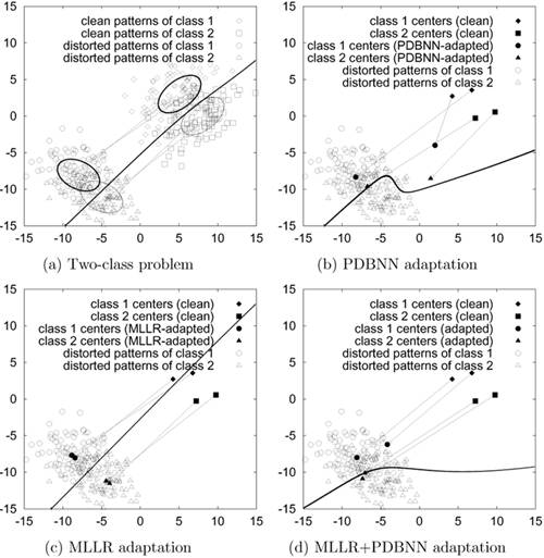
The clean models were adapted using the methods explained before, and the results are shown in Figures 9.14(b) through 9.14(d). In Figures 9.14(b), 9.14(c), and 9.14(d), the markers ♦ and ▪ represent the centers of the clean models and • and ▴ represent the centers of the adapted models. The arrows indicate the adaptation of model centers, and the thick curves show the equal-error decision boundaries derived from the adapted models. For PDBNN-adaptation (Figure 9.14(b)), two clean GMMs were trained independently using the clean patterns of each class. The distorted patterns of both classes were used to adapt the clean models using PDBNN's reinforced learning. For MLLR-adaptation (Figure 9.14(c)), a clean GMM was trained using the clean patterns of both classes, which was followed by the estimation of MLLR parameters using the clean GMM and the distorted patterns of both classes. The two clean GMMs corresponding to the two classes were then transformed using the estimated MLLR parameters. For the cascaded MLLR-PDBNN adaptation (Figure 9.14(d)), the clean models were first transformed by MLLR, then PDBNN adaptation was performed on the adapted models to obtain the final model.

A comparison between Figure 9.14(b) and Figure 9.14(c) reveals that while PDBNN-adaptation can transform only some of the model centers to the region of the distorted clusters, MLLR-based adaptation can transform all of the centers of the clean GMMs to a region around the distorted clusters. By cascading MLLR transformation and PDBNN adaptation, all of the centers of the clean GMMs can be transformed to a region within the distorted clusters before the decision boundary is fine-tuned. The adaptation capability of cascading MLLR and PDBNN is also demonstrated in the speaker verification evaluation described in Section 9.4.3.

Applications to Channel Compensation

A recently proposed handset selector has been adopted (see Handset Selector section and references [226, 227, 352, 353]) to identify the most likely handset given an utterance. Specifically, H GMMs, , as shown in Figure 9.12, were independently trained using the distorted speech recorded from the corresponding phone handsets. During recognition, the claimant's features, y(t), t = 1, ..., T, were fed to all GMMs. The most likely handset k* is selected by the Maxnet, as illustrated in Figure 9.12.

For PDBNN adaptation, the precomputed PDBNN-adapted speaker model and background model corresponding to the k*-th handset were used for verification. For MLLR adaptation, the precomputed MLLR adaptation matrix (W^k*) for the k*-th handset was used to transform the clean speaker model (M_s) to the MLLR-adapted speaker model . The same matrix was also used to transform the clean background model (M_b) to the MLLR-adapted background model . For MLLR+PDBNN adaptation, the precomputed MLLR adaptation matrix (W^k*) for the k*-th handset was first used to transform the clean models (M_s, M_b) to the MLLR-adapted model (, ). Then, PDBNN adaptation was performed on the MLLR-adapted models to obtain the MLLR+PDBNN adapted models (, ). These models are to be used for verifying the claimant.

Experimental Evaluation

Enrollment Procedures

Similar to SFT, the HTIMIT corpus was used in the evaluation. Speakers in the HTIMIT corpus were divided into a speaker set (100 speakers) and an impostor set (50 speakers). Each speaker in the speaker set was assigned a 32-center GMM (M_s) characterizing his or her own voice. For each speaker model, training feature vectors were derived from the SA and SX utterances of the corresponding speaker. A 64-center GMM universal background model (M_b), which was trained using all of the SA and SX utterances from all speakers in the speaker set, was used to normalize the speaker scores (see Eq. 9.4.16). Utterances from the head-mounted microphone (senh) were considered to be clean and were used for creating the speaker models and background models. The feature vectors were twelfth-order MFCCs computed every 14ms using a Hamming window of 28ms.

Environment Adaptation

For PDBNN-based adaptation, the clean speaker model (M_s) and clean background model (M_b) described before were used as the initial models for GS training. The SA and SX utterances of the target speaker and the background speakers (excluding the target speaker) from a phone handset were used as positive and negative training patterns, respectively. Hence, for each target speaker, a handset-dependent speaker model and a handset-dependent background model were created for each handset (including the head-mounted microphone used for enrollment).

For MLLR-based adaptation, a single, full transformation matrix is used to compensate for the "mismatch" between two environments. Specifically, a clean background model (M_b) was trained using the clean speech of all speakers in the speaker set. Then, the speech data from another handset were used to estimate a transformation matrix corresponding to that handset using MLLR. This procedure was repeated for all handsets in the HTIMIT corpus.

For MLLR+PDBNN adaptation, both MLLR transformation and PDBNN globally supervised training were applied to compensate for the mismatched conditions. First, MLLR was used to transform the clean speaker model (M_s) and the clean background model (M_b) to handset-specific models. PDBNN globally supervised training were then applied to the handset-specific models. The handset-specific SA and SX utterances of the target speaker and the background speakers (excluding the target speaker) were used as the training patterns in the PDBNN supervised training.

The MLLR+PDBNN+SFT adaptation is identical to MLLR+PDBNN adaptation except that the former uses stochastically transformed speaker features in the PDBNN globally supervised training. Specifically, the clean speaker patterns from the senh handset were transformed using SFT to obtain a set of artificial, handset-specific training patterns. With SFT, the necessity of handset-specific speaker patterns for PDBNN training is eliminated. Because handset-specific speech patterns for the background speakers are easily obtainable, performing SFT on the background speaker's speech is unnecessary.

A preliminary evaluation was performed to compare the performance of MLLR transformation using 5, 20, and 100 speakers to estimate the adaptation matrices Ws. Although the performance improves with the number of speakers, the computation time also increases with the total number of training patterns. The MLLR transformation matrices used in the following experiments were estimated using 20 and 100 speakers. Experiments have also been conducted using SFT [226], Hnorm [303], and Tnorm [14] for comparison. The parameters for SFT were estimated using the same 20 and 100 speakers, as in PDBNN model adaptation and MLLR model transformation. For Hnorm, the speech patterns derived from the handset-specific utterances of 49 same-gender (same as the client speaker), nontarget speakers were used to compute the handset-dependent means and standard deviations. As a result, each client speaker model is associated with 10 handset-dependent score means and variances. These means and variances were used during verification to normalize the claimant's scores. For Tnorm [14], verification utterances were fed to all of the 99 nontarget speaker models to calculate the mean and variance parameters. These parameters were then used to normalize the speaker scores.

Verification Procedures

During verification, a pattern sequence Y derived from each of the SI sentences of the claimant was fed to the GMM-based handset selector . Handset-dependent speaker and background models/adaptation matrix were selected according to the handset selector's output (see Figure 9.12). The test utterance was then fed to an adapted speaker model and an adapted background model to obtain the score

Equation 9.4.16

where Ψ ¸ { PDBNN, MLLR, PDBNN+MLLR, PDBNN+MLLR+SFT } represents the type of adaptation used to obtain the adapted models. S(Y) was compared with a global, speaker-independent threshold to make a verification decision. In this work, the threshold was adjusted to determine the equal error rates (EERs).

Results and Discussions

Figure 9.15 and Table 9.9 show the results of different environment adaptation approaches, including CMS, Tnorm [14], Hnorm [303], PDBNN adaptation, SFT [226], MLLR, MLLR+PDBNN, and MLLR+PDBNN+ SFT adaptation. All error rates were based on the average of 100 target speakers and 50 impostors.

Table 9.9. EER achieved by CMS, Tnorm, Hnorm, PDBNN, SFT, MLLR, MLLR+PDBNN, and MLLR+PDBNN+SFT adaptations. Note: CMS and Tnorm do not require the handset selector. All results were based on 100 target speakers and 50 impostors. The MLLR and SFT transformation matrices were estimated using 20 and 100 speakers (denoted as –20 and –100, respectively) in the speaker set. For MLLR+PDBNN and MLLR+PDBNN+SFT, 100 speakers were used to created the transformation matrices.

Adaptation Method	Equal Error Rate (%)
	cb1	cb2	cb3	cb4	ell	el2	el3	el4	pt1	senh	Ave.
CMS	8.21	8.50	21.20	15.40	8.15	11.20	11.49	8.85	10.56	6.79	11.03
Tnorm	8.88	8.94	22.58	14.94	9.30	9.78	10.40	8.64	8.51	5.54	10.74
Hnorm	7.30	6.98	13.81	10.42	7.42	9.40	10.32	7.62	9.34	7.06	8.96
PDBNN-100	7.72	8.48	10.02	9.66	6.72	11.59	8.64	9.59	8.99	3.01	8.44
SFT-20	4.18	3.61	17.64	11.81	4.93	7.24	7.82	3.85	6.64	3.60	7.13
SFT-100	4.28	3.61	17.55	11.06	4.81	7.60	7.34	3.87	6.12	3.65	6.98
MLLR-20	4.69	3.34	17.23	10.21	5.52	7.35	9.66	4.76	8.84	3.54	7.51
MLLR-100	4.52	3.14	15.17	9.58	4.79	7.60	6.46	4.84	6.94	3.69	6.67
SFT-20+Hnorm	4.18	3.61	17.64	11.81	4.93	7.24	7.87	3.85	6.64	3.60	7.13
MLLR+PDBNN (100)	4.30	3.12	10.16	6.89	5.01	6.84	6.36	4.87	6.53	3.43	5.75
MLLR+PDBNN+SFT (100)	4.21	3.01	12.86	7.65	4.97	5.65	6.05	4.26	5.46	3.43	5.75

Evidently, all cases of environment adaptation show significant reduction in error rates when compared to CMS. In particular, MLLR+PDBNN and MLLR+PDBNN+SFT adaptation achieve the largest error reduction. Table 9.9 also demonstrates that model-based adaptation and feature-based transformation (SFT) are comparable in terms of error rate reduction (ERR).

Although PDBNN adaptation uses discriminative training to adapt the model parameters to fit the new environment, the results show that using PDBNN adaptation alone is not desirable because its performance is not as good as that of MLLR adaptation. This may be due to the intrinsic design of PDBNNs (i.e., the supervised reinforced/antireinforced learning of PDBNNs are designed for fine-tuning the decision boundaries by slightly adjusting the model centers responsible for the mis-classifications). As a result, some of the centers will not be adapted at all. Because only misclassified data are used for adaptation and their amount is usually small after LU training, moving all of the centers from the clean space to the environmentally distorted space may be difficult. Alternatively, MLLR adaptation finds a transformation matrix to maximize the likelihood of the adaptation data. Thus, moving all of the model centers to the environmentally distorted space is much easier.

PDBNN adaptation requires speaker-specific training data from all possible handsets that the users can use. MLLR adaptation, on the other hand, only requires some environment-specific utterances to estimate the global transformation matrices, which requires much less training data; better still, the utterances do not necessarily need to be produced by the same client speaker. PDBNN adaptation also requires additional training for the inclusion of new speakers because the new speaker models and the background models should be adapted using gradient descent to environment-specific models. On the other hand, for MLLR adaptation, transformation is applied to new speaker models and background models once the MLLR transformation matrices have been estimated.

The results also demonstrate that SFT and MLLR achieve a comparable amount of error reduction. A comparison between SFT-20 and MLLR-20 (where the training utterances of 20 speakers were used to estimate the transformation parameters) reveals that SFT performs slightly better when the amount of training data is small. This is because the number of free parameters in feature transformation is much less than that of MLLR. However, the performance of SFT quickly saturates when the total number of training patterns increases, as indicated in SFT-100 and MLLR-100. While MLLR requires much more data to estimate the global transformation matrices robustly, its performance is better than that of SFT when sufficient training data are available.

The performances of the proposed environment adaptation approaches were also compared with that of Hnorm [303] and Tnorm [14]. As shown in Table 9.9, both methods outperform the classical CMS; however, the improvement is not as significant as SFT and MLLR. Recall that both Hnorm and Tnorm work on the likelihood-ratio score space using two normalization parameters only (bias and scale). SFT and MLLR, on the other hand, aim to compensate the mismatch effect at the feature space and model space. Both methods can translate and scale the components of feature vectors or models' centers. Because the number of free parameters in SFT and MLLR is much larger than that of Hnorm and Tnorm, SFT and MLLR are more effective provided that the free parameters can be estimated correctly.

Because SFT and Hnorm work on different spaces (SFT transforms the speech features in the feature space while Hnorm performs score normalization in the score space), these two techniques were also combined to see whether further improvement could be obtained. The results (third row—"SFT-20+Hnorm"—from bottom in Table 9.9) show that no improvement was obtained when compared with SFT-20. A possible reason is that the score distributions of clients and impostors after SFT are already well separated; as a result, handset normalization cannot improve the performance further in the score space.

Although it may not be desirable to use PDBNN's reinforced learning alone, it is amenable to the fine-tuning of the MLLR-transformed centers. This is evident from the second row from the bottom of Table 9.9, where error reductions of 13.8% with respect to MLLR-100 and 31.9% with respect to PDBNN-100 were achieved. The main reason behind these error reductions is that MLLR can transform the clean model centers to the region of distorted clusters; these initial centers give a better seed for reinforced learning.

For MLLR+PDBNN+SFT adaptation, an average EER of 5.75% is achieved (bottom row of Table 9.9), which is identical to that of the MLLR+PDBNN adaptation. Bear in mind that MLLR+PDBNN adaptation requires speaker-specific and handset-specific training data, whereas MLLR+PDBNN+SFT adaptation requires handset-specific training data only. Having the same EER means that MLLR+PDBNN+SFT adaptation is a better method.

To compare the computation complexity, the training and verification time of different adaptation approaches were measured. The simulations were performed on a Pentium IV 2.66GHz CPU. The measurements were based on 30 speakers and 50 impostors in the HTIMIT corpus and the total CPU time running the whole task was recorded. The training time is composed of two parts: systemwise computation time and enrollment computation time. The systemwise computation time represents the time to carry out the tasks that only need to be performed once, including computation of the MLLR transformation matrices and background model training. The enrollment computation time represents the time to enroll a new speaker and to adapt his or her models. It was determined by taking the average enrollment time of 30 client speakers using seven utterances per speaker. The verification time is the time taken to verify a claimant based on a single utterance. It was determined by taking the average verification time of 80 claimants (30 client speakers and 50 impostors) using three utterances per claimant.

Table 9.10 shows the training and verification time for Hnorm, Tnorm, PDBNN-100, MLLR-100, MLLR+PDBNN-100, and MLLR+PDBNN+SFT-100. Evidently, PDBNN adaptation requires extensive computational resources during enrollment because a handset-specific speaker model and a handset-specific background model were created for each speaker for each acoustic environment. The results also show that computing the MLLR transformation matrices requires an extensive amount of computational resources. Hnorm requires only a small amount of resources for enrollment because it needs to estimate only the score mean and score variance. Tnorm also requires a small amount of computation during enrollment. However, because all of the normalization parameters are estimated from the scores of all speaker models during verification, Tnorm is very computation intense during verification. All other adaptations can achieve near realtime performance during verification.

Table 9.10. Total training and verification time used by different adaptation approaches. The training time is composed of two parts: systemwise computation time, which represents the time to carry out tasks that only need to be performed once, and enrollment computation time. The systemwise tasks include the computation of the MLLR transformation matrices and background model training. The enrollment tasks are the time required to enroll a new speaker and adapt his or her models.

Adaptation Method	Training Time		Verification Time (seconds)
	Systemwise Computation (seconds)	Enrollment Computation (seconds)
Hnorm	324.30	240.78	2.48
Tnorm	324.30	0.96	37.54
PDBNN-100	324.30	8489.54	1.20
MLLR- 100	130713.30	0.96	0.38
MLLR+PDBNN-100	130713.30	2561.74	1.59
MLLR+PDBNN+SFT-100	130713.30	5157.77	1.27

Although both Hnorm and Tnorm work on the likelihood-ratio score space, they have different complexities when it comes to training and testing. The main computation for Hnorm lies in the training phase and is proportional to the total number of nontarget utterances because these utterances are fed to the speaker and background models to calculate the nontarget scores, which in turn are used to calculate the normalization parameters. Once the Hnorm parameters have been calculated, rapid verification can be achieved. For Tnorm, on the other hand, verification is computationally intense and the amount of computation is proportional to the total number of speaker models used for deriving the normalization scores. For a better estimation of Tnorm parameters, a large number of scores are required, which in turn require a large number of speaker models. This can greatly lengthen verification time.

9.4.4. Out-of-Handset Rejection

The handset selector defined by Eq. 9.4.14 simply selects the most likely handset from a set of known handsets even for speech coming from an unseen handset. In addition, the approach requires a handset database containing all types of handsets that users are likely to use; at least two reasons make this requirement difficult to fulfill in practical situations. First, because there are so many types of phone handsets on the market, it is almost impossible to include all of them in the handset database. Second, new handset models are released every few months, which means the handset database must be updated frequently to keep it current. If a claimant uses a handset that has not been included in the handset database, the verification system may identify the handset incorrectly, resulting in verification error.

To address the preceding problems, combining SFT and a GMM-based handset selector with out-of-handset (OOH) rejection capability for assisting speaker verification has been proposed [352, 354]. Specifically, each handset in the database of the handset selector is assigned a set of transformation parameters. During verification, the handset selector determines whether the handset used by the claimant is one of the handsets in the database. If so, the selector identifies the most likely handset and transforms the distorted vectors according to the transformation parameters of the identified handset. Otherwise, the selector identifies the handset as "unseen" and processes the distorted vectors by cepstral mean subtraction (CMS). Figure 9.16 illustrates the idea of incorporating OOH rejection into the handset selector.

The Jensen Difference

For each utterance, the selector either identifies or rejects the handset. The decision is based on the following rule:

Equation 9.4.17

where , is the Jensen difference [39, 360] between and —whose values will be discussed next—and ϕ is a decision threshold. can be computed as

Equation 9.4.18

where called the Shannon entropy, is defined by

Equation 9.4.19

where z_i is the i-th component of .

The Jensen difference has a nonnegative value and can be used to measure the divergence between two vectors. If all elements of and are similar, will have a small value. On the other hand, if the elements of and are different, the value of will be large. For the case where is identical to , becomes 0. Therefore, Jensen difference is an ideal candidate for measuring the divergence between two n-dimensional vectors.

The handset selector here uses the Jensen difference to compare the probabilities of a test utterance produced by the known handsets. Let Y = {yt = 1, ..., T} be a sequence of feature vectors extracted from an utterance recorded by an unknown handset, and l_h(y_t) be the log-likelihood of observing the pattern y_t, given it is generated by the h-th handset (i.e., l_h(y_t) = log p(Y_t|Гh). Hence, the average log-likelihood of observing the sequence Y, given it is generated by the h-th handset, is

Equation 9.4.20

For each vector sequence X, = [α_l α₂ ... α_H]^T is created with each of its element

Equation 9.4.21

representing the probability that the test utterance is produced by the h-th handset such that and α_h > 0 for all h. If all the elements of are similar, the probabilities of the test utterance produced by each handset are close, and it is difficult to identify which handset the utterance comes from. On the other hand, if the elements of are not similar, some handsets will be more likely than others to produce the test utterance. In this case, being able to identify the handset from which the utterance is recorded is likely.

The similarity among the elements of is determined by the Jensen difference between (with the elements of vector defined in Eq. 9.4.21) and a reference vector , where , h = 1, …, H. A small Jensen difference indicates that all elements of are similar, while a large value means that the elements of are different.

During verification, when the selector finds that the Jensen difference is greater than or equal to the threshold ϕ, the selector identifies the most likely handset according to Eq. 9.4.14, and the transformation parameters corresponding to the selected handset are used to transform the distorted vectors. On the other hand, when is less than ϕ, the selector considers the sequence Y to be coming from an unseen handset. In the latter case, the distorted vectors will be processed differently, as shown in Figure 9.16.

Similarity and Dissimilarity among Handsets

Because the divergence-based handset classifier is designed to reject dissimilar, unseen handsets, handsets that are either similar to one of the seen handsets or dissimilar to all seen handsets must be used for evaluation. The similarity and dissimilarity among the handsets can be observed from a confusion matrix. Given N utterances (denoted as Y^(i,n), n = 1,...,N) from the i-th handset and the GMM of the j-th handset (denoted as Гj), the average log-likelihood of the j-th handset is

Equation 9.4.22

where is the likelihood of the model Г_j given the t-th frame of the n-th utterance recorded from the i-th handset, and T_n is the number of frames in Y^(i,n).

To facilitate comparison among the handsets, the average log-likelihood is normalized according to

Equation 9.4.23

where P_max and P_min are respectively the maximum and minimum log-likelihoods found in the matrix (i.e., P_max = max_i,j P_ij and P_min = min_i,j P_ij). As a result, the largest normalized log-likelihood has a value of 1.00, and the smallest has a value of 0.00. Each of the 's, 0 ≤ i,j ≤ H, corresponds to an element in the confusion matrix. This matrix enables the identification of those handsets with similar (or dissimilar) characteristics. For example, a large value of suggests that the i-and j-th handsets are similar; on the other hand, a small value of P_ij implies that they are different.

A confusion matrix containing the normalized log-likelihoods of the 10 handsets is shown in Table 9.11. The utterances of these handsets were obtained from 100 speakers in the HTIMIT corpus. Note that the diagonal elements are the largest among all other elements in their respective rows. This is because the log-likelihood of a handset given the utterances from the same handset should be the largest.

Table 9.11. Confusion matrix containing the normalized log-likelihoods of 10 different handsets. The normalized log-likelihoods were found using Eq. 9.4.23, and have a range between 0.00 and 1.00. Entries with a large value implies that the handset corresponding to that row and the handset corresponding to that column have similar characteristics; a small value implies that the characteristics between the two handsets are different. Elements in bold on the diagonal are the largest because the i-th GMM should give the largest log-likelihood for utterances from the i-th handset.

Normalized Log-Likelihood of Handset ()
Utterances from Handset (i)	Handset Model (Гi)
	cb1	cb2	cb3	cb4	ell	el 2	el3	el4	pt1	senh
cb1	0.80	0.66	0.38	0.41	0.64	0.51	0.63	0.47	0.52	0.53
cb2	0.61	0.76	0.22	0.36	0.45	0.33	0.56	0.55	0.39	0.54
cb3	0.72	0.62	1.00	0.86	0.70	0.55	0.65	0.64	0.60	0.58
cb4	0.66	0.62	0.76	0.94	0.65	0.43	0.59	0.56	0.51	0.56
ell	0.56	0.45	0.13	0.21	0.73	0.49	0.54	0.35	0.52	0.48
el2	0.57	0.47	0.01	0.02	0.61	0.81	0.69	0.46	0.64	0.43
el3	0.60	0.57	0.20	0.27	0.61	0.63	0.77	0.53	0.57	0.59
el4	0.40	0.54	0.25	0.28	0.40	0.37	0.50	0.75	0.28	0.40
pt1	0.60	0.53	0.20	0.27	0.64	0.66	0.69	0.47	0.84	0.51
senh	0.43	0.49	0.00	0.11	0.46	0.24	0.50	0.30	0.29	0.71

The confusion matrix in Table 9.11 demonstrates the similarity and dissimilarity among all handsets. For example, a value of 1.00 means very similar and a value of 0.00 implies very dissimilar. However, the matrix does not show how similar a particular handset is to another handset. The normalized log-likelihood differences provide this information:

Equation 9.4.24

Table 9.12 depicts a matrix containing the values of . The table clearly shows that the cb1 handset is similar to cb2, el1, and el3 because their normalized log-likelihood differences with respect to handset cb1 are small (≤ 0.17). On the other hand, it is likely that cb1 has characteristics different from those of handsets cb3 and cb4 because their normalized log-likelihood differences are large (≥ 0.39).

Table 9.12. Normalized log-likelihood differences of 10 handsets (see Eq. 9.4.24). Entries with small (large) value means that the corresponding handsets are similar (different).

	Normalized Log- Likelihood Difference
Utterances from Handset (i)	Handset Model (Гi)
	cb1	cb2	cb3	cb4	ell	el2	el3	el4	pt1	senh
cb1	0.00	0.14	0.42	0.39	0.16	0.29	0.17	0.33	0.28	0.27
cb2	0.15	0.00	0.54	0.40	0.31	0.43	0.20	0.21	0.37	0.22
cb3	0.28	0.38	0.00	0.14	0.30	0.45	0.35	0.36	0.40	0.42
cb4	0.28	0.32	0.18	0.00	0.29	0.51	0.35	0.38	0.43	0.38
Ell	0.17	0.28	0.60	0.52	0.00	0.24	0.19	0.38	0.21	0.25
el2	0.24	0.34	0.80	0.79	0.20	0.00	0.12	0.35	0.17	0.38
el3	0.17	0.20	0.57	0.50	0.16	0.14	0.00	0.24	0.20	0.18
el4	0.35	0.21	0.50	0.47	0.35	0.38	0.25	0.00	0.47	0.35
pt1	0.24	0.31	0.64	0.57	0.20	0.18	0.15	0.37	0.00	0.33
senh	0.28	0.22	0.71	0.60	0.25	0.47	0.21	0.41	0.42	0.00

The confusion matrix in Table 9.12 labels some handsets as unseen, while the remaining are considered seen handsets. These two categories of handsets—seen and unseen—will be used to test the OOH rejection capability of the proposed handset selector.

Experimental Evaluations

In this experiment, the OOH rejection capability of the handset selector was studied. Different approaches were applied to integrate the OOH rejection into a speaker verification system, and utterances from "seen" and "unseen" handsets were used to test the resulting system. The following section discusses how the seen and unseen handsets were chosen for testing the OOH rejection capability of the handset selector. The discussion is followed by a detailed description of the approaches to integrating the OOH rejection into a speaker verification system.

Selection of Seen and Unseen Handsets

When a claimant uses a handset that has not been included in the handset database, the characteristics of this unseen handset may be different from all of those in the database, or its characteristics may be similar to one or a few handsets in the database. Therefore, it is important to test the handset selector under two scenarios: (1) unseen handsets with characteristics different from those of the seen handsets, and (2) unseen ones with characteristics similar to seen handsets.

Seen and unseen handsets with different characteristics. Table 9.12 shows that the cb3 and cb4 handsets are similar. In the table, the normalized log-likelihood difference in row cb3, column cb4, has a value of 0.14 and the normalized log-likelihood difference in row cb4, column cb3, is 0.18; both of these entries have small values. On the other hand, these two handsets (cb3 and cb4) are not similar to all other handsets because the log-likelihood differences in the remaining entries of row cb3 and row cb4 are large. Therefore, in the first part of the experiment, the cb3 and cb4 handsets were used as the unseen ones, and the other eight handsets were used as the seen handsets.

Seen and unseen handsets with similar characteristics. The confusion matrix in Table 9.12 shows that the el2 handset is similar to el3 and pt1 since their normalized log-likelihood differences with respect to el2 are small (i.e., 0.12 and 0.17, respectively, in row el2 of the table). It is also likely that cb3 and cb4 have similar characteristics as stated in the previous paragraph. Therefore, if cb3 and el2 are used as the unseen handsets, and the remaining are left as the seen handsets, it will be possible to find some seen handsets (e.g., cb4, el3, and pt1) that are similar to the two unseen ones. In the second part of the experiment, cb3 and el2 are used as the unseen handsets and the other eight handsets are used as the seen ones.

Approaches to Incorporating OOH Rejection into Speaker Verification

Three different approaches to integrating the handset selector into a speaker verification system were investigated; they are denoted as Approach I, Approach II, and Approach III, and are detailed in Table 9.13. In the experiment, nine handsets (cb1-cb4, el1-el4, and pt1) and one Sennheizer head-mounted microphone (senh) from HTIMIT [304] were used as the testing handsets. These handsets were divided into the seen and unseen categories, as described before. Speech from the senh handset was used for enrolling speakers, and speech from the other nine handsets was used for verifying speakers. The enrollment and verification procedures were identical to those in Section 9.4.2.

Table 9.13. Three different approaches to integrating OOH rejection into a speaker verification system.

Approach	OOH Rejection Method	Rejection Handling
I	None	N/A
II	Euclidean distance-based	Use CMS-based speaker models to verify the rejected utterances
III	Divergence-based	Use CMS-based speaker models to verify the rejected utterances

Approach I: Handset selector without OOH rejection. In this approach, if test utterances from an unseen handset are fed to the handset selector, the selector is forced to choose an incorrect handset and a wrong set of transformation parameters will be used to transform the distorted vectors. The handset selector consists of eight 64-center Gaussian mixture models (GMMs) corresponding to the eight seen handsets. Each GMM was trained with the distorted speech recorded from the corresponding handset. Also, for each handset, a set of feature transformation parameters v that transform speech from the corresponding handset to the enrolled handset (senh) were computed (see Section 9.4.2). Note that utterances from the unseen handsets were not used to create any GMM models.

During verification, a test utterance was fed to the GMM-based handset selector, which then chose the most likely one from the eight handsets according to Eq. 9.4.14, with H = 8. Then, the transformation parameters corresponding to the k*-th handset were used to transform the distorted speech vectors for speaker verification.

Approach II: Handset selector with Euclidean distance-based OOH rejection and CMS. In this approach, OOH rejection was implemented based on the Euclidean distance between two vectors: a vector (with the elements of vector defined in Eq. 9.4.21) and a reference vector = [r₁ r₂ … r_H]^T, where , i = 1, ..., H. The vector distance D (,) between and is

Equation 9.4.25

The selector then identifies the most likely handset or rejects the handset using the decision rule:

Equation 9.4.26

where ζ is a decision threshold. Specifically, for each utterance, the handset selector determines whether the utterance is recorded from one of the eight known handsets according to Eq. 9.4.26. If so, the corresponding transformation is used to transform the distorted speech vectors; otherwise, cepstral mean subtraction (CMS) is used to compensate for the channel distortion.

Approach III: Handset selector with divergence-based OOH rejection and CMS. This approach uses a handset selector with divergence-based OOH rejection capability. Specifically, for each utterance, the handset selector determines whether it is recorded from one of the eight known handsets by making an accept or a reject decision according to Eq. 9.4.17. For an accept decision, the handset selector selects the most likely one from the eight handsets and uses the corresponding transformation parameters to transform the distorted speech vectors. For a reject decision, CMS was applied to the utterance rejected by the handset selector to recover the clean vectors from the distorted ones.

Scoring Normalization

Recovered vectors were fed to a 32-center GMM speaker model. Depending on the handset selector's decision, the recovered vectors were either fed to a GMM-based speaker model without CMS (M_s) to obtain the score (log p(Y|M_s)) or fed to a GMM-based speaker model with to obtain the CMS-based score . In either case, the score was normalized according to

Equation 9.4.27

where M_b and are the 64-center GMM background model without CMS and with CMS, respectively. S(Y) was compared with a threshold to make a verification decision. In this work, the threshold for each speaker was adjusted to determine an equal error rate (EER).

Results and Discussions

The experimental results using the cb3 and cb4 handsets as the unseen handsets are summarized in Table 9.14.^[6] All of the stochastic feature transformations used in this experiment were of second-order. For Approach II, the threshold ζ (Eq. 9.4.26) for the decision rule used in the handset selector was set to 0.25, while for Approach III, the threshold ϕ (Eq. 9.4.17) for the handset selector was set to 0.06. These threshold values were found to produce the best result empirically.

^[6] Table 9.12 and the discussion in the Similarity and Dissimilarity among Handsets section demonstrate that cb3 and cb4 are different from all other handsets.

Table 9.14. Results for seen and unseen handsets with different characteristics. Note: EERs (in %) achieved by the baseline, CMS, and the three handset selector integration approaches are shown here (see Table 9.13 for integration methods). Handsets cb3 and cb4 were used as the unseen handsets. The enrollment handset is senh. The average handset identification accuracy is 98.25%. Note that the baseline and CMS do not require the handset selector.

Compensation Method	Integration Method	Equal Error Rate (%)
		cb1	cb2	cb3	cb4	ell	el2	el3	el4	pt1	Ave.	senh
Baseline	N/A	8.15	7.01	25.78	18.08	5.99	15.06	7.86	14.02	9.75	12.41	2.99
CMS	N/A	6.42	5.71	13.33	10.17	6.15	9.29	9.59	7.18	6.81	8.29	4.66
2nd-order SFT	Approach I	4.14	3.56	19.02	18.41	3.54	6.78	6.38	4.72	4.69	7.92	2.98
2nd-order SFT	Approach II	4.39	3.99	13.37	12.34	4.29	6.57	8.77	4.74	5.06	7.05	2.98
2nd-order SFT	Approach III	4.17	3.91	13.35	12.30	4.54	6.46	7.60	4.69	5.23	6.92	2.98

In addition, Table 9.14 shows that Approach I substantially reduces the average EER. The average goes down to 7.92%, as compared to 12.41% for the baseline and 8.29% for CMS. However, no reductions in EERs for the "unseen" handsets (i.e., cb3 and cb4) were found. The EER of cb3 using this approach is even higher than the one obtained by the CMS method. Handset cb4's EER is even higher than that of the baseline. Therefore, it can be concluded that using an incorrect set of transformation parameters can degrade the verification performance when the characteristics of the unseen handset are different from the seen handsets.

Table 9.14 also shows that Approach II is able to achieve a satisfactory performance. With the Euclidean distance-based OOH rejection, there were 365 and 316 rejections out of 450 test utterances for the two unseen handsets (cb3 and cb4), respectively. As a result of these rejections, the EERs of cb3 and cb4 were reduced to 13.37% and 12.34%, respectively. These errors are significantly lower than those achievable by Approach I. Nevertheless, some utterances from the seen ones were rejected by the handset selector, causing a higher EER for other "seen" handsets. Therefore, OOH rejection based on Euclidean distance has limitations.

As shown in the last row of Table 9.14, Approach III achieves the lowest average EER. The reduction in EERs is also the most significant for the two unseen handsets. In an ideal situation with this approach, all utterances of the unseen handsets will be rejected by the selector and processed by CMS, and the EERs of the unseen handsets are reduced to those achievable by the CMS method. In the experiment, 369 and 284 rejections were obtained out of 450 test utterances for cb3 and cb4, respectively. As a result of these rejections, the EERs corresponding to handsets cb3 and cb4 decrease to 13.35% and 12.30%, respectively; neither are significantly different from the EERs achieved by the CMS method. Although this approach may cause the EERs of the seen handsets (except for el2 and el4) to be slightly higher than those achieved by Approach I, it is a worthwhile tradeoff because its average EER is still lower than that of Approach I. Approach III also reduces the EERs of the two seen handsets (el2 and el4) because some of the incorrectly identified utterances in Approach I were rejected by the handset selector in Approach III. Using CMS to recover the distorted vectors of these utterances allows the verification system to recognize speakers correctly.

Figure 9.17 shows the distribution of the Jensen difference for the cb1 seen handset and the cb3 unseen handset. The vertical dash-dot line defines the decision threshold used in the experiment (i.e., ϕ = 0.06). According to Eq. 9.4.17, the handset selector accepts the handsets for Jensen differences greater than or equal to the decision threshold (i.e., the region to the right of the dash-dot line) and rejects the handset for Jensen differences less than the decision threshold (i.e., the region to the left of the dash-dot line). For cb1, only a small area under its Jensen difference distribution is inside the rejection region, which means that few utterances from this handset were rejected by the selector—out of 450 test utterances in the experiment, only 14 were rejected. On the other hand, a large portion of cb3's distribution is inside the rejection region. As a result, most of the utterances from this unseen handset are rejected by the selector—out of 450 utterances, 369 were rejected.

To better illustrate the detection performance of the verification system, the DET curves are plotted, as introduced in Martin et al. [233], for the three approaches. The speaker detection performance, using the cb1 seen handset and the cb3 unseen handset in verification sessions, are shown in Figures 9.18 and 9.19, respectively. The five DET curves in each figure represent five different methods of processing the speech, and each curve was obtained by averaging the DET curves of 100 speakers. Note that the curves are almost straight because each DET curve is constructed by averaging the DET curves of 100 speakers, resulting in a normal distribution. Appendix B illustrates how the average DET curves were obtained.

The EERs obtained from the curves in Figure 9.18 correspond to the values in column cb1 of Table 9.14, and the EERs in Figure 9.19 correspond to the values in column cb3. Due to interpolation errors, there are slight discrepancies between the EERs obtained from the figures and those shown in Table 9.14.

In addition, Figures 9.18 and 9.19 show that Approach III achieves satisfactory performance for both seen and unseen handsets. In Figure 9.18, using Approach III, the DET curve for the cb1 seen handset is close to the curve achieved by Approach I. In Figure 9.19, using Approach III, the DET curve for the cb3 unseen handset is close to the curve achieved by the CMS method. Therefore, by applying Approach III (with divergence-based OOH rejection) to the speaker verification system, the error rates of a seen handset can be reduced to values close to that achievable by Approach I (without OOH rejection); the error rates of an unseen handset, the characteristics of which are different from all the seen ones, can be reduced to values close to that achievable by the CMS method.

The experimental results using cb3 and el2 as the unseen handsets are summarized in Table 9.15.^[7] Again, all the stochastic transformations (STs) used in this experiment were second-order. For Approach II, the threshold ζ (Eq. 9.4.26) for the decision rule used in the handset selector was set to 0.25. For Approach III, the threshold ϕ used by the handset selector was set to 0.05. These threshold values were found to produce the best results empirically.

^[7] According to Table 9.12 and the arguments in the Similarity and Dissimilarity among Handsets section, cb3 is similar to cb4, and handset el2 is similar to el3 and pt1.

Table 9.15. Results for seen and unseen handsets with similar characteristics. Note: EER (in %) achieved by the baseline, CMS, and the three handset selector integration approaches are shown here (see Table 9.13 for integration methods). Handsets cb3 and el2 were used as the unseen handsets. The enrollment handset is senh. The average handset identification accuracy is 98.38%. Notice that the baseline and CMS do not require the handset selector.

Compensation Method	Integration Method	Equal Error Rate (%)
		cb1	cb2	cb3	cb4	ell	el2	el3	el4	pt1	Ave.	senh
Baseline	N/A	8.15	7.01	25.78	18.08	5.99	15.06	7.86	14.02	9.75	12.41	2.99
CMS	N/A	6.42	5.71	13.33	10.17	6.15	9.29	9.59	7.18	6.81	8.29	4.66
2nd-order ST	Approach I	4.14	3.56	13.35	6.75	3.53	9.82	6.37	4.72	4.69	6.33	2.98
2nd-order ST	Approach II	4.14	3.56	13.30	6.75	4.08	9.46	6.59	4.70	4.73	6.37	2.98
2nd-order ST	Approach III	4.14	3.56	13.10	6.75	3.48	9.63	6.20	4.72	4.69	6.25	2.98

Table 9.15 shows that Approach I can achieve a satisfactory performance. Its average equal error rate is significantly smaller than that of the baseline and ceptral mean subtraction method. In addition, the EERs of the two unseen handsets, cb3 and el2, have values close to those of the CMS method even without out-of-handset rejection. This occurs because the characteristics of cb3 are similar to those of the cb4 seen handset, and those of el2 are similar to those of the el3 and pt1 seen handsets.

Therefore, when utterances from cb3 are fed to the handset selector, it chooses cb4 as the most likely handset in most cases (out of 450 test utterances from cb3, 446 were identified as coming from cb4). Because the transformation parameters of cb3 and cb4 are close, the recovered vectors (despite using an incorrect set of transformation parameters) can still be correctly recognized by the verification system. A similar situation occurs when utterances from handset cb2 are fed to the selector. In this case, the transformation parameters of either el3 or pt1 are used to recover the distorted vectors (out of 450 test utterances from el2, 330 were identified as coming from el3, and 73 utterances were identified as being from pt1).

In addition, Table 9.15 shows that the performance of Approach II is not satisfactory. Although this approach can bring further reduction in EERs for the two unseen handsets (as a result of 21 rejections for cb3 and 11 rejections for el2), the cost is a higher average EER over Approach I.

Results in Table 9.15 also show that Approach III, once again, achieves the best performance. Its average EER is the lowest, and further reduction in EERs of the two unseen handsets (cb3 and el2) was obtained. For the el2 handset, there were only two rejections out of 450 test utterances because most of the utterances were considered to be from the el3 or pt1 seen handset. With such a small number of rejections, the EER of el2 is reduced to 9.63%, which is close to the 9.29% of the CMS method. The EER of the cb3 handset is even lower than that obtained by the CMS method. Out of the 450 utterances from cb3, 428 were identified as being from cb4, 20 were rejected, and only two were incorrectly identified by the handset selector. Because most of the utterances were either transformed by the transformation parameters of the cb4 handset or recovered using CMS, its EER is reduced to 13.10%.

Figure 9.20 shows the distribution of the Jensen difference for the cb1 seen handset and the cb3 unseen handset. The vertical dash-dot line defines the decision threshold used in the experiment (i.e., ϕ = 0.05). For cb1, all of the area under its probability density curve of the Jensen difference is in the handset acceptance region, which means that no rejection was made by the handset selector (In the experiment, all utterances from the cb1 handset were accepted by the handset selector.) For cb3, a large portion of the Jensen difference distribution is also in the handset acceptance region. This occurs because the characteristics of the cb3 handset are similar to those of cb4; as a result, few rejections were made by the selector (only 20 out of 450 utterances were rejected in the experiment).

The speaker detection performance for the seen handset cb1 and the unseen handset cb3 is shown in Figures 9.21 and 9.22, respectively. The EERs measured from the DET curves in Figure 9.21 correspond to the values in column cb1 of Table 9.15, and the EERs from Figure 9.22 correspond to the values in column cb3. Again, the slight discrepancy between the measured EERs and the EERs in Table 9.15 is due to interpolation error.

Figures 9.21 and 9.22 show that Approach III can achieve satisfactory performance for both seen and unseen handsets. In particular, Figure 9.21 shows that when Approach III was used, the DET curve of the cb1 seen handset overlaps the curve obtained by Approach I. This means that Approach III is able to keep the EERs of the seen handsets at low values. In Figure 9.22, using Approach III, the DET curve of the cb3 unseen handset is slightly on the left of the curve obtained by the CMS method, resulting in slightly lower error rates. Therefore, by applying Approach III to the speaker verification system, the error rates of a seen handset can be reduced to values close to those achievable by Approach I. On the other hand, the error rates of an unseen handset, with characteristics similar to some of the seen handsets, can be reduced to values close to or even lower than the values achievable by the CMS method.